Classifying pairs with trees
for supervised biological network inference
†
Marie Schrynemackers,
∗aLouis Wehenkel,
aM. Madan Babu,
band Pierre Geurts
aReceived Xth XXXXXXXXXX 20XX, Accepted Xth XXXXXXXXX 20XX First published on the web Xth XXXXXXXXXX 20XX
DOI: 10.1039/b000000x
Networks are ubiquitous in biology, and computational approaches have been largely investigated for their inference. In partic-ular, supervised machine learning methods can be used to complete a partially known network by integrating various measure-ments. Two main supervised frameworks have been proposed: the local approach, which trains a separate model for each network node, and the global approach, which trains a single model over pairs of nodes. Here, we systematically investigate, theoretically and empirically, the exploitation of tree-based ensemble methods in the context of these two approaches for biological network inference. We first formalize the problem of network inference as classification of pairs, unifying in the process homogeneous and bipartite graphs and discussing two main sampling schemes. We then present the global and the local approaches, extending the later for the prediction of interactions between two unseen network nodes, and discuss their specializations to tree-based ensemble methods, highlighting their interpretability and drawing links with clustering techniques. Extensive computational experiments are carried out with these methods on various biological networks that clearly highlight that these methods are competitive with existing methods.
1
Introduction
In biology, relationships between biological entities (genes, proteins, transcription factors, micro-RNA, diseases, etc.) are
often represented by graphs (or networks‡). In theory, most of
these networks can be identified from lab experiments but in practice, because of the difficulties in setting up these experi-ments and their costs, we often have only a very partial knowl-edge of them. Because more and more experimental data be-come available about biological entities of interest, several re-searchers took an interest in using computational approaches to predict interactions between nodes in order to complete ex-perimental predictions.
When formulated as a supervised learning problem, net-work inference consists in learning a classifier on pairs of nodes. Mainly two approaches have been investigated in the literature to adapt existing classification methods for this
prob-lem.1 The first one, that we call the global approach,
con-siders this problem as a standard classification problem on an input feature vector obtained by concatenating the feature
vectors of each node from the pair.1 The second approach,
called local,2,3trains a different classifier for each node
sep-† Electronic Supplementary Information (ESI) available: Implementation and computational issues, supplementary performance curves, and illustration of interpretability of trees. See DOI: 10.1039/b000000x/
aDepartment of EE and CS & GIGA-R, University of Li`ege, Belgium; E-mail:
bMRC Laboratory of Molecular Biology, Cambridge, UK.
‡ In this paper, the terms network and graph will refer to the same thing.
arately, aiming at predicting its direct neighbors in the graph. These two approaches have been mainly exploited with sup-port vector machine (SVM) classifiers. In particular, several kernels have been proposed for comparing pairs of nodes in
the global approach4,5 and the global and local approaches
can be related for specific choices of this kernel.6A number
of papers applied the global approach with tree-based
ensem-ble methods, mainly Random Forests,7for the prediction of
protein-protein8–11 and drug-protein12interactions,
combin-ing various feature sets. Besides the local and global meth-ods, other approaches for supervised graph inference includes,
among others, matrix completion methods,13 methods based
on output kernel regression,14,15Random Forests-based
simi-larity learning,16and methods based on network properties.17
In this paper, we would like to systematically investigate, theoretically and empirically, the exploitation of tree-based ensemble methods in the context of the local and global ap-proaches for supervised biological network inference. We first formalize biological network inference as the problem of classification on pairs, considering in the same framework homogeneous graphs, defined on one kind of nodes, and bi-partite graphs, linking nodes of two families. We then de-fine the general local and global approaches in the context of this formalization, extending in the process the local ap-proach for the prediction of interactions between two unseen network nodes. The paper discusses in details the specializa-tion of these approaches to tree-based ensemble methods. In particular, we highlight their high potential in terms of
inter-pretability and draw connections between these methods and unsupervised (bi-)clustering methods. Experiments on several biological networks show the good predictive performance of the resulting family of methods. Both the local and the global approaches are competitive with however an advantage for the global approach in terms of predictive performance and for the local approach in terms of compactness of the inferred models. The paper is structured as follows. Section 2 first defines the general problem of supervised network inference and cast it as classification problem on pairs. Then, it presents two generic approaches to address it and their particularization for tree en-sembles. Section 3 reports experiments with these methods on several homogeneous and bipartite biological networks. Sec-tion 4 concludes and discusses future work direcSec-tions. Addi-tional experimental results and implementation details can be found in the supplementary material.
2
Methods
We first formalize the problem of supervised network infer-ence and discuss the evaluation of these methods in Section 2.1. We then present in Section 2.2 two generic approaches to address it. Section 2.3 discusses the specialization of these two approaches in the context of tree-based ensemble meth-ods.
2.1 Supervised network inference as classification on
pairs
For the sake of generality, we consider bipartite graphs that connect two sets of nodes. The graph is thus defined by an
adjacency matrix Y , where each entry yi j is equal to one if
there is an edge between the nodes nirand ncj, and zero if not.
The subscripts r and c are used to differentiate the two sets of nodes and stand respectively for row and column of the adja-cency matrix Y . Moreover, each node (or sometimes pair of nodes) is described by a feature representation, i.e. typically a vector of numerical values, denoted by x(n) (see Figure 1 for an illustration). Homogeneous graphs defined on only one family of nodes can be obtained as special cases of this gen-eral framework by considering only one set of nodes and thus
a square and symmetric adjacency matrix.18
In this context, the problem of supervised network inference can be formulated as follows (see Figure 1):
Given a partial knowledge of the adjacency matrix
Y of the target network, find the best possible
pre-dictions of the missing or unknown entries of this matrix by exploiting the feature description of the network nodes.
In this paper, we address this problem as a supervised
classi-fication problem on pairs18. A learning sample, denoted LSp,
n
j cn
irx
(n
ir)
x
(n
j c)
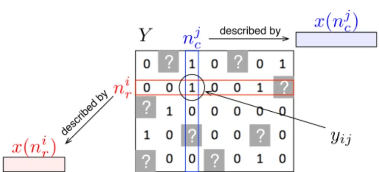
Y
y
ij described by described by?
?
?
?
?
?
?
?
Fig. 1 A network can be represented by an adjacency matrix Y where each row and each column correspond to a specific node, with potentially different families of nodes associated with rows and columns. Each node is furthermore described by a feature vector, with potentially different features describing row and column nodes. For instance, row nodes nircan be proteins and column nodes n
j ccan be drugs, with the adjacency matrix encoding drug-protein
interactions. Proteins could be described by their PFAM domains and drugs by features encoding their chemical structure. Supervised network inference then consists in inferring missing entries in the adjacency matrix (question marks in gray) from known entries (in white) by exploiting node features.
is constructed as the set of all pairs of nodes that are known to interact or not (i.e., the known entries in the adjacency ma-trix). The input variables used to describe these pairs are the feature vectors of the two nodes in the pair. A classification
model f (i.e. a function associating a label in{0, 1} to each
combination of the input variables) can then be trained from
LSpand used to predict the missing entries of the adjacency
matrix.
The evaluation of the predictions of supervised network in-ference methods requires special care. Indeed, all pairs are not as easy as the others to predict: it is typically much more diffi-cult to predict pairs that involve nodes for which no examples
of interactions are provided in the learning sample LSp. As a
consequence, to get a complete assessment of a given method, one needs to partition the predictions into different families, depending on whether the nodes in the tested pair are
repre-sented or not in the learning set LSp, and then to perform a
separate evaluation within each family.18
To formalize this, let us denote by LScand LSr the nodes
from the two sets that are present in LSp(i.e. which are
in-volved in some pairs in LSp) and by T Scand T Sr (where T S
stands for Test Set) the nodes that are unseen in LSp. The pairs
of nodes to predict (i.e., outside LSp) can be divided into the
following four families (where S1× S2denotes the cartesian
product between sets S1and S2and S1\ S2their difference):
• (LSr× LSc) \ LSp: predictions of (unseen) pairs between
two nodes which are represented in the learning sample. • LSr× T Scor T Sr× LSc: predictions of pairs between one
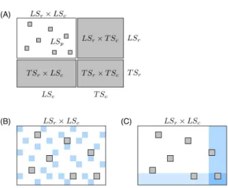
Fig. 2 (A) Schematic representation of known and unknown pairs in the network adjacency matrix. Known pairs (that can be interacting or not) are in white and unknown pairs, to be predicted, are in gray. Rows and columns of the adjacency matrix have been rearranged to highlight the four families of unknown pairs described in the text: LSr× LSc, LSr× T Sc, T Sr× LSc, and T Sr× T Sc. (B) Schematic representation of CV on pairs: In this procedure, we randomly divide the pairs of the learning sample into two groups : we learn a model on the pairs from the white area, and test it on the pairs from the blue area. The CV on pairs evaluates LS× LS predictions. Pairs in gray represent unknown pairs that do not take part to the CV. (C) Schematic representation of CV on nodes: In this procedure, we randomly divide the nodes of each set (relative to the rows and the columns) into two groups : we learn a model on the pairs from the white area, and test it on the pairs from the blue area. The CV on pairs evaluates LS× T S, T S × LS and T S × T S predictions.
node represented in the learning sample and one unseen node.
• T Sr× T Sc: predictions of pairs between two unseen
nodes.
These families of pairs are represented in the adjacency matrix in Figure 2A. Thereafter, to simplify the notations, we denote
the four families as LS× LS, LS × T S, T S × LS and T S × T S.
In the case of an homogeneous undirected graph, only three
sets can be defined as the two sets LS× T S and T S × LS are
confounded.18
Prediction performances are expected to differ between
these four families. Typically, one expects that T S× T S pairs
will be the most difficult to predict since less information is available at training about the corresponding nodes. These predictions will then be evaluated separately in this work, as
suggested in several publications18,19. They can be evaluated
by performing two kinds of cross-validation (CV): A first CV procedure on pairs of nodes (denoted “CV on pairs”) to
evalu-(A) (B) (C)
Fig. 3 Schematic representation of the training data. In the global approach (A) the features vectors are concatenated, in the local approach with single output (B) one function is learnt for each node, and in the local approach with multiple output (C) one function is learnt for one family of nodes and one function for the other one.
ate LS× LS predictions (see Figure 2B) and a second CV
pro-cedure on nodes (denoted “CV on nodes”) to evaluate LS×T S,
T S× LS and T S × T S predictions (see Figure 2C).18
2.2 Two different approaches
In this section, we present the two generic, local and global, approaches we have adopted for dealing with classification on pairs. We will discuss in Section 2.3 their practical implemen-tation in the context of tree-based ensemble methods. In the presentation of the approaches, we will assume that we have at our disposal a classification method that derives its clas-sification model from a class conditional probability model.
Denoting by f a classification model, we will denote by fp
(i.e., with superscript p) the corresponding class conditional
probability function. f(x) is the predicted class (0 or 1)
as-sociated with some input x, while fp(x) (resp. 1 − fp(x)) is
the predicted probability (∈ [0, 1]) of the input x being of class
1 (resp. 0). Typically, f(x) is obtained from fp(x) by
com-puting f(x) = 1( fp(x) > p
th) for some user-defined threshold
pth∈ [0, 1], where pthcan be adjusted to find the best tradeoff
between sensitivity and specificity according to the applica-tion needs.
2.2.1 Global Approach. The most straightforward
ap-proach for dealing with the problem defined in Section 2.1 is
to apply a classification algorithm on the learning sample LSp
of pairs to learn a function fglob on the cartesian product of
the two input spaces (resulting in the concatenation of the two input vectors of the nodes of the pair). Predictions can then be computed straightforwardly for any new unseen pair from the function. (Figure 3A)
In the case of an homogeneous graph, the adjacency ma-trix Y is a symmetric square mama-trix. We will introduce two adaptations of the approach to handle such graphs. First, for each pair(nr,nc) in the learning sample, the pair (nc,nr) will
constraint on the classification method, this will not ensure
however that the learnt function fglobwill be symmetric in its
arguments. To make it symmetric, we will compute a new
class conditional probability model fglob,symp from the learned
one fglobp as follows:
fglob,symp (x1,x2) =
fglobp (x1,x2) + fglobp (x2,x1)
2 ,
where x1and x2are the input feature vectors of the nodes in
the pair to be predicted.
2.2.2 Local Approach. The idea of the local approach,2
is to build a separate classification model for each node, try-ing to predict its neighbors in the graph from the known graph
around this node. More precisely, for a given node nc∈ LSc,
a new learning sample LS(nc) is constructed from the
learn-ing sample of pairs LSp, comprising all the pairs that involve
the target node nc and the feature vectors associated to the
interacting nodes nr. It can then be used to learn a
classifica-tion model fnc, which can be exploited to make a prediction
for any new pair involving nc. By symmetry, the same
strat-egy can be adopted to learn a classification model fnrfor each
node nr∈ LSr. (Figure 3B)
These two sets of classifiers can then be exploited to make
LS× T S and T S × LS types of predictions. For pairs (nr,nc) in
LS× LS, two predictions can be obtained: fnc(nr) and fnr(nc).
We propose to simply combine them by an arithmetic average of the corresponding class conditional probability estimates.
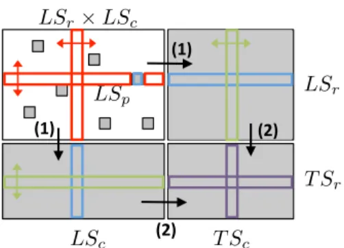
As such, the local approach is in principle not able to make directly predictions for pairs of nodes(nr,nc) ∈ T S × T S
(be-cause LS(nr) = LS(nc) = /0 for nr∈ T Sr and nc∈ T Sc). We
nevertheless propose to use the following two-steps procedure to learn a classifier for a node nr∈ T Sr(see Figure 4):
• First, learn all classifiers fncfor nodes nc∈ LSc
(equiva-lent to the completion of the columns in Figure 4), • Then, learn a classifier fnfr from the predictions given by
the models fnctrained in the first step (equivalent to the
completion of the rows in Figure 4).
Again by symmetry, the same strategy can be applied to obtain models fnfc for the nodes nc∈ T Sc. A prediction is then
ob-tained for a pair(nr,nc) in T S × T S by averaging the class
con-ditional probability predictions of both models fnf ,pr and f
f ,p nc .
A related two-step procedure has been proposed by Pahikkala
et al.20for learning on pairs with kernel methods.
Note that to derive the learning samples needed to train models fnfcand f
f
nr in the second step, one requires to choose
a threshold on the predicted class conditional probability esti-mates (to turn these probabilities into binary classes). In our experiments, we will set this threshold in such a way that the
LSr× T Sc T Sr× T Sc T Sr× LSc LSr× LSc LSc LSr T Sr T Sc LS p !"# !"#$ !%#$ !"#$ !%#$
Fig. 4 The local approach needs two steps to learn a classifier for an unseen node: (1) first, we predict LS× T S and T S × LS interactions, and (2) from these predictions, we predict T S× T S interactions.
proportion of edges versus non edges in the predicted
subnet-works in LS× T S and T S × LS is equal to the same proportion
within the original learning sample of pairs.
This strategy can be specialized to the case of a homoge-neous graph in a straightforward way. Only one class of clas-sifiers fnand fnf are trained for nodes in LS and in T S
respec-tively (using the same two-step procedure as in the asymmetric
case for the second). LS× LS and T S × T S predictions are still
obtained by averaging two predictions, one for each node of the pair.
2.3 Tree-based ensemble methods
Any method could be used as a base classifier for the two ap-proaches. In this paper, we propose to evaluate the use of tree-based ensemble methods in this context. We first briefly describe these methods and then discuss several aspects re-lated to their use within the two generic approaches.
2.3.1 Description of the methods. A decision tree21
rep-resents an input-output model by a tree whose interior nodes are each labeled with a (typically binary) test based on one input feature and each terminal node is labeled with a value of the output. The predicted output for a new instance is de-termined as the output associated to the leaf reached by the instance when it is propagated through the tree starting at the root node. A tree is built from a learning sample of input-output pairs, by recursively identifying, at each node, the test that leads to a split of the nodes sample into two subsamples that are as pure as possible in terms of their output values.
Single decision trees typically suffer from high variance, which makes them not competitive in terms of accuracy. This problem is circumvented by using ensemble methods that gen-erate several trees and then aggregate their predictions. In this paper, we exploit one particular ensemble method called
each tree in the ensemble by selecting at each node the best among K randomly generated splits. In our experiments, we use the default setting of K, equal to the square root of the total number of candidate attributes.
One interesting features of tree-based methods (single and ensemble) is that they can be extended to predict a vectorial
output instead of a single scalar output.23We will exploit this
feature of the method in the context of the local approach be-low.
2.3.2 Global approach. The global approach consists in
building a tree from the learning sample of all pairs. Each split of the resulting tree will be based on one of the input features
coming from either one of the two input feature vectors, x(nr)
or x(nc). The tree growing procedure can thus be interpreted
as interleaving the construction of two trees: one on the row nodes and one on the column nodes. Each leaf of the result-ing tree is thus associated with a rectangular submatrix of the
graph adjacency matrix Y (reduced to the pairs in LSr× LSc)
and the construction of the tree is such that the pairs in this submatrix should be, as far as possible, either all connected or all disconnected (see Figure 5 for an illustration).
2.3.3 Local approach. The use of tree ensembles in the
context of the local approach is straightforward. We will nev-ertheless compare two variants. The first one builds a separate model for each row and column nodes as presented in Sec-tion 2.2. The second method exploits the ability of tree-based methods to deal with multiple outputs (vector outputs) to build only two models, one for the row nodes and one for the col-umn nodes (Figure 3C). We assume that the learning sample
has been generated by sampling two subsets of nodes LSrand
LSc and that the full adjacency matrix is observed between
these two sets (as in Figure 2C). The first model related to the
column nodes is built from a learning sample LS(nc)
compris-ing all the observed pairs, and the feature vectors associated
to the row nodes nr. It can then be used to learn a
classifi-cation model, which can be exploited to make the predictions
of the interaction profiles of all nodes ncpresent in the
learn-ing sample of pairs LSp. By symmetry, the same strategy can
be adopted to learn classification model for the row nodes nr.
The two-steps procedure can then be applied to build the two
models required to make T S× T S predictions.
This approach has the advantage of requiring only four tree ensemble models in total instead of one model for each poten-tial node in the case of the single output approach. It can how-ever only be used when the complete submatrix is observed
for pairs in LS× LS, since tree-based ensemble method cannot
cope with missing output values.
2.3.4 Interpretability. One main advantage of tree-based
methods is their interpretability, directly through the tree structure in the case of single tree models and through
fea-! !!! ! !!! ! ! !!! !!! !!! (A) (B)
Fig. 5 Both the global approach (A) and the local approach with multiple output (B) can be interpreted as carrying out a biclustering of the adjacency matrix. Each subregion is characterized by conjunctions of tests based on the input features. In this graph, xc,i (resp. xr,i) denotes the ith feature of the column (resp. row) node. Note that in the case of the global approach, the representation is only illustrative. The adjacency submatrices corresponding to the tree leaves can not be necessarily rearranged as contiguous rectangular submatrices covering the initial adjacency matrix.
ture importance rankings in the case of ensembles.24 Let us
compare both approaches along this criterion.
In the case of the global approach, as illustrated in Fig-ure 5A, the tree that is built partitions the adjacency matrix
(more precisely, its LSr× LSc part) into rectangular regions.
These regions are defined such that pairs in each region are either all connected or all disconnected. The region is further-more characterized by a path in the tree (from the root to the leaf) corresponding to tests on the input features of both nodes of the pair.
In the case of the local multiple output approach, one of the two trees partitions the rows and the other tree partitions the columns of the adjacency matrix. Each partitioning is carried out in such a way that nodes in each subpartition has a similar connectivity profiles. The resulting partitioning of the adja-cency matrix will thus follow a checkerboard structure with also only connected or disconnected pairs in the obtained sub-matrix, as far as possible (Figure 5B). Each submatrix will be furthermore characterized by two conjunctions of tests, one based on row inputs and one based on column inputs. These two methods can thus be interpreted as carrying out a
biclus-tering25of the adjacency matrix where the biclustering is
how-ever directed by the choice of tests on the input features. An concrete illustration can be found in Figure 6 and in the sup-plementary material.
In the case of the local single output approach, the partition-ing is more fine-grained as it can be different from one row or column to another. However in this case, each tree gives an
in-Proteins 20 40 60 80 20 40 60 80 100 120 140 160 180 1. SC1C(N)CCCC1 2. >= 1 Co 3. N-S-C:C
4. >= 1 saturated or aromatic nitrogen-containing ring size 8’ 5. >= 1 unsaturated non-aromatic carbon-only ring size 10’ ’C(∼Br)(∼H) 6. >= 1 any ring size 7
7. >= 1 saturated or aromatic carbon-only ring size 6 8. C(∼C)(∼H)(∼N)
9. O-C:C-O-[♯1] 10. N-H 11. Nc1cc(Cl)ccc1 12. O-C:C-O
1. Eukaryotic-type carbonic anhydrase 2. Oestrogen receptor
3. 7 transmembrane receptor (rhodopsin family)
Fig. 6 Illustration of the interpretability of multiple-output decision-tree on a drug-protein interaction network. We zoomed in the rectangular subregion with the highest number of interactions, and presented the list of drug and protein features associated to this region. See the supplementary material for more details about the procedures.
Table 1 Summary of the six datasets used in the experiments. Network Network size Number Number
of edges of features Homogen. PPI 984×984 2438 325 networks EMAP 353×353 1995 418 MN 668×668 2782 325 Bipartite ERN 154×1164 3293 445/445 networks SRN 113×1821 3663 9884/1685 DPI 1862×1554 4809 660/876
terpretable characterization of the nodes which are connected to the node from which the tree was built.
When using ensembles, the global approach provides a global ranking of all features from the most to the less rele-vant. The local multiple output approach provides two sepa-rate rankings, one for the row features and one for the column features and the local single output approach gives a separate ranking for each node. All variants are therefore complemen-tary from an interpretability point of view.
3
Experiments
In this section, we carried out a large scale empirical evalua-tion of the different methods described in Secevalua-tion 2.2 on six real biological networks, three homogeneous graphs and three bipartite graphs. Results on four additional (drug-protein) net-works can be found in the supplementary material. Our goal with these experiments is to assess the relative performances of the different approaches and to give an idea of the perfor-mance one could expect from these methods on biological net-works of different nature. Section 3.4 provides a comparison with existing methods from the literature.
3.1 Datasets
The first three networks correspond to homogeneous
undi-rected graphs and the last three to bipartite graphs. The
main characteristics of the datasets are summarized in Table 1. The adjacency matrices used in the experiments, the lists of nodes and lists of features can be downloaded at
http://www.montefiore.ulg.ac.be/˜schrynemackers/datasets.html
3.1.1 Protein-protein interaction network (PPI). This
network26has been compiled from 2438 high confidence
in-teractions highlighted between 984 S. cerivisiae proteins. The input features used for the predictions are a set of expression data, phylogenetic profiles and localization data that totalizes 325 features. This dataset has been used in several studies before.13,14,27
3.1.2 Genetic interaction network (EMAP). This
negative epistatic interactions. Inputs29consists in measures of growth fitness of yeast cells relative to deletion of each gene separately, and in 418 different environments.
3.1.3 Metabolic network (MN). This network30is
com-posed of 668 S. cerivisiae enzymes connected by 2782 edges. There is an edge between two enzymes when these two en-zymes catalyse successive reactions. The input feature vectors are the same as those used in the PPI network.
3.1.4 E. coli regulatory network (ERN). This bipartite
network31 connects transcription factors (TF) and genes of
E. coli. It is composed of 1164 genes regulated by 154 TF.
There is a total of 3293 interactions. The input features31are
445 expression values.
3.1.5 S. cerevisiae regulatory network (SRN). This
net-work32connects TFs and their target genes from E. coli. It is
composed of 1855 genes regulated by 113 TFs and totalizing 3737 interactions. The input features are 1685 expression val-ues.33–36For genes, we concatenated motifs features37to the expression values.
3.1.6 Drug-protein interaction network (DPI). This
network38is related to human and connect a drug with a
pro-tein when the drug targets the propro-tein. This network holds 4809 interactions involving 1554 proteins and 1862 drugs. The input features are a binary vectors coding for the pres-ence or abspres-ence of 660 chemical substructures for each drug, and the presence or absence of 876 PFAM domains for each protein.38
3.2 Protocol
In our experiments, LS× LS performances in each network are
measured by 10 fold cross-validation (CV) across the pairs of nodes, as illustrated in Figure 2B. For robustness, results are
averaged over 10 runs of 10 fold CV. LS× T S, T S × LS and
T S× T S predictions are assessed by performing a 10 times
10 fold CV across the nodes, as illustrated in Figure 2C. The different algorithms return class conditional probability es-timates. To assess our models independently of a
particu-lar choice of discretization threshold Pth on these estimates,
we vary this threshold and output in each case the resulting precision-recall curve and the resulting ROC curve. Meth-ods are then compared according to the total area under these curves, denoted AUPR and AUROC respectively (the higher the AUPR and the AUROC, the better), averaged over the 10 folds and the 10 CV runs. For all our experiments, we use ensembles of 100 extremely randomized trees with default pa-rameter setting.22
As highlighted by several studies,39in biological networks,
nodes of high degree have a higher chance to be connected to any new node. In our context, this means that we can expect
0 0.5 1 0 0.2 0.4 0.6 0.8 1 LS × LS Recall Pre ci si o n Global Local so 0 0.5 1 0 0.2 0.4 0.6 0.8 1 Recall Pre ci si o n LS × TS Global Local so Local mo 0 0.5 1 0 0.2 0.4 0.6 0.8 1 Recall Pre ci si o n TS × TS Global Local so Local mo
Fig. 7 Precision-recall curves for metabolic network: higher is the number of nodes of a pair present in the learning set, better will be the prediction for this pair.
that the degree of a node will be a good predictor to infer new interactions involving this node. We want to assess the impor-tance of this effect and provide a more realistic baseline than the usual random guess performance. To reach this goal, we evaluate the AUROC and AUPR scores when using the sum
of the degrees of each node in a pair to rank LS× LS pairs and
when using the degree of the nodes belonging to the LS to rank
T S× LS or LS × T S pairs. AUROC and AUPR scores will be
evaluated using the same protocol as hereabove. As there is no
information about the degrees of nodes in T S× T S pairs, we
will use random guessing as a baseline for the scores of these predictions (corresponding to an AUROC of 0.5 and an AUPR equal to the proportion of interactions among all nodes pairs).
3.3 Results
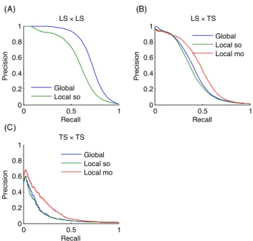
We discuss successively the results on the three homogeneous networks and then on the three bipartite networks.
3.3.1 Homogeneous graphs. AUPR and AUROC values
are summarized in Table 2 for the three methods: global, lo-cal single output, and lolo-cal multiple output. The last row on each dataset is the baseline result obtained as described in 3.2. Figure 7 shows the precision-recall curves obtained by the dif-ferent approaches on MN, for the three difdif-ferent protocols. Similar curves for the two other networks can be found in the supplementary material.
Table 2 Areas under curves for homogeneous networks.
Precision-Recall (AUPR) ROC (AUC)
LS× LS LS× T S T S× T S LS× LS LS× T S T S× T S PPI Global 0.41 0.22 0.10 0.88 0.84 0.76 Local so 0.28 0.21 0.11 0.85 0.82 0.73 Local mo - 0.22 0.11 - 0.83 0.72 Baseline 0.13 0.02 0.00 0.73 0.74 0.50 EMAP Global 0.49 0.36 0.23 0.90 0.85 0.78 Local so 0.45 0.35 0.24 0.90 0.84 0.79 Local mo - 0.35 0.23 - 0.85 0.80 Baseline 0.30 0.13 0.03 0.87 0.80 0.50 MN Global 0.71 0.40 0.09 0.95 0.85 0.69 Local so 0.57 0.38 0.09 0.92 0.83 0.68 Local mo - 0.45 0.14 - 0.85 0.71 Baseline 0.05 0.04 0.01 0.75 0.70 0.50
pairs are clearly the easiest to predict, followed by LS× T S
pairs and T S× T S pairs. This ranking was expected from
pre-vious discussions. Baseline results in the case of LS× LS and
LS× T S predictions confirm that nodes degrees are very
in-formative: baseline AUROC values are much greater than 0.5 and baseline AUPR values are also significantly higher than the proportion of interactions among all pairs (0.005, 0.03, and 0.01 respectively for PPI, EMAP, and MN), especially in the
case of LS× LS predictions. Nevertheless, our methods are
better than these baselines in all cases. On the EMAP net-work, the difference in terms of AUROC is very slight but the difference in terms of AUPR is important. This is typical of highly skewed classification problems, where precision-recall curves are known to give a more informative picture of the
performance of an algorithm than ROC curves.40
All tree-based approaches are very close on LS× T S and
T S× T S pairs but the global approach has an advantage over
the local one on LS× LS pairs. The difference is important
on the PPI and MN networks. For the local approach, the performance of single and multiple output approaches are in-distinguishable, except with the metabolic network where the multiple output approach gives better results. This is in line with the better performance of the global versus the local ap-proach on this problem, as indeed both the global and the local multiple output approaches grow a single model that can po-tentially exploit correlations between the outputs. Notice that the multiple output approach is not feasible when we want to
predict LS× LS pairs, as we are not able to deal with missing
output values in multiple output decision trees.
3.3.2 Bipartite graphs. AUPR and AUROC values are
summarized in Table 3 (see the supplementary material for ad-ditional results on four DPI subnetworks). Figure 8 shows the precision-recall curves obtained by the different approaches
on ERN for the four different protocols. Curves for the 6 other networks can be found in the supplementary material. 10 times 10-fold CV was used as explained in Section 3.2. Nevertheless, two difficulties appeared in the experiments per-formed on the DPI network. First, the dataset is larger than the others, and the 10-fold CV was replaced by 5-fold CV to reduce the computational space et time burden. Second, the feature vectors are binary and the randomization of the thresh-old (in Extra-Tree algorithm) cannot lead to diversity between the different trees of the ensemble. So we used bootstrapping to generate the training set of each tree.
Like for the homogeneous networks, higher is the number of nodes of a pair present in the learning set, better are the predictions, i.e., AUPR and AUROC values are significantly
decreasing from LS× LS to T S × T S predictions. On the ERN
and SRN networks, performances are very different for the
two kinds of LS× T S predictions that can be defined, with
much better results when generalizing over genes (i.e., when the TF of the pair is in the learning sample). On the other
hand, on the DPI network, both kinds of LS× T S predictions
are equally well predicted. These differences are probably due in part to the relative numbers of nodes of both kinds in the learning sample, as there are much more genes than TFs on ERN and SRN and a similar number of drugs and proteins in the DPI network. Differences are however probably also re-lated to the intrinsic difficulty of generalizing over each node family, as on the four additional DPI networks (see the sup-plementary material), generalization over drugs is most of the time better than generalization over proteins, irrespectively of the relative numbers of drugs and proteins in the training net-work. Results are most of the time better than the baselines
(based on nodes degrees for LS× LS and LS × T S predictions
and on random guessing for T S× T S predictions). The only
Table 3 Areas under curves for bipartite networks.
Precision-Recall (AUPR) ROC (AUC)
LS× LS LS× T S T S× LS T S× T S LS× LS LS× T S T S× LS T S× T S
ERN(TF - gene) Global 0.78 0.76 0.12 0.08 0.97 0.97 0.61 0.64
Local so 0.76 0.76 0.11 0.10 0.96 0.97 0.61 0.66 Local mo - 0.75 0.09 0.09 - 0.97 0.61 0.65 Baseline 0.31 0.30 0.02 0.02 0.86 0.87 0.52 0.50 SRN(TF - gene) Global 0.23 0.27 0.03 0.03 0.84 0.84 0.54 0.57 Local so 0.20 0.25 0.02 0.03 0.80 0.83 0.53 0.57 Local mo - 0.24 0.02 0.03 - 0.83 0.53 0.57 Baseline 0.06 0.06 0.03 0.02 0.79 0.78 0.51 0.50
DPI(drug - protein) Global 0.14 0.05 0.11 0.01 0.76 0.71 0.76 0.67
Local so 0.21 0.11 0.08 0.01 0.85 0.72 0.72 0.57 Local mo - 0.10 0.08 0.01 - 0.72 0.71 0.60 Baseline 0.02 0.01 0.01 0.01 0.82 0.63 0.68 0.50 0 0.5 1 0 0.2 0.4 0.6 0.8 1 Recall Pre ci si o n LS × LS Global Local so 0 0.5 1 0 0.2 0.4 0.6 0.8 1 Recall Pre ci si o n LS × TS Global Local so Local mo 0 0.5 1 0 0.2 0.4 0.6 0.8 1 Recall Pre ci si o n TS × L Global L 0 0.5 1 0 0.2 0.4 0.6 0.8 1 Recall Pre ci si o n TS × TS Global Local so Local mo
Fig. 8 Precision-recall curves for E.coli regulatory network (TF vs genes): a prediction is easier to do if the TF belongs to the learning set than if the gene belongs to.
and when predicting T S× T S pairs on SRN and DPI.
The three approaches are very close to each other. Unlike on homogeneous graphs, there is no strong difference between
the global and the local approach on LS× LS predictions: it is
slightly better in terms of AUPR on ERN and SRN but worse on DPI. The single and multiple output approaches are also very close, both in terms of AUPR and AUROC. Similar re-sults are observed on the four additional DPI networks.
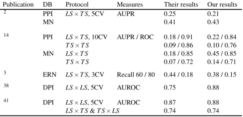
3.4 Comparison with related works
In this section, we compare our methods with several other network inference methods from the literature. To ensure a fair comparison and avoid errors related to the reimplemen-tation and tuning of each of these methods, we choose to re-run our algorithms in similar settings as in related papers. All comparison results are summarized in Table 4 and discussed below.
3.4.1 Homogeneous graphs. A local approach with
sup-port vector machines was developed to predict the PPI and
MN networks2and showed to be superior to several previous
works13,27 in terms of performance. The authors only
con-sider LS× T S predictions and used 5-fold CV. Although they
exploited yeast-two-hybrid data as additional features for the prediction of the PPI network, we obtain very similar perfor-mances with the local multiple output approach (see Table 4).
Another method14that uses ensembles of output kernel trees
also infers the MN and PPI networks with the same input data. With the global approach, we obtain similar or inferior results in terms of AUROC but much better results in terms of AUPR, especially on the MN data.
3.4.2 Bipartite graphs. SVM have been used to predict
Table 4 Comparison with related works on the different networks.
Publication DB Protocol Measures Their results Our results
2 PPI LS× T S, 5CV AUPR 0.25 0.21
MN 0.41 0.43
14 PPI LS× T S, 10CV AUPR / ROC 0.18 / 0.91 0.22 / 0.84
T S× T S 0.09 / 0.86 0.10 / 0.76 MN LS× T S 0.18 / 0.85 0.45 / 0.85 T S× T S 0.07 / 0.72 0.14 / 0.71 3 ERN LS× T S, 3CV Recall 60 / 80 0.44 / 0.18 0.38 / 0.15 38 DPI LS× LS, 5CV AUROC 0.75 0.88 41 DPI LS× LS, 5CV AUROC 0.87 0.88 LS× T S & T S × LS 0.74 0.74
interactions between known TFs and new genes (LS× T S).
Authors evaluated their performances by the precision at 60% and 80% recall respectively, estimated by 3-fold CV (ensuring that all genes belonging to a same operon are always in the same fold). Our results with the same protocol (and the local multiple output variant) are very close although slightly less good. The DPI network was predicted using sparse
canoni-cal correspondence analyze (SCCA)38and with the global
ap-proach and L1 regularized linear classifiers41 using as input
features all possible products of one drug feature and one
pro-tein feature. Only LS× LS predictions are considered in the
first paper, while the second one differentiates “pair-wise CV”
(our LS× LS predictions) and “block-wise CV” (our LS × T S
and T S× LS predictions). As shown in Table 4, we obtain
better results than SCCA and similar results as in L1 SVM.
Additional comparisons are presented in the supplementary material on the four DPI subnetworks.
Globally, these comparisons show that tree-based methods are competitive on all six networks. Moreover, it has to be noticed that (1) no other method has been tested over all these problems, and (2) we have not tuned any parameters of the Extra-Trees method. Better performances could be achieved
by changing, for example, the randomization scheme,7 the
feature selection parameter K, or the number of trees.
4
Discussion
We explored tree-based ensemble methods for biological net-work inference, both with the local approach, which trains a separate model for each network node (single output) or each node family (multiple output), and with the global approach, which trains a single model over pairs of nodes. We carried out experiments on ten biological networks and compared our results with those from the literature. These experiments show that the resulting methods are competitive with the state of the
art in terms of predictive performance. Other intrinsic advan-tages of tree-based approaches include their interpretability, through single tree structure and ensemble-derived feature im-portance scores, as well as their almost parameter free nature and their reasonable computational complexity and storage re-quirement.
The global and local approaches are close in terms of
accu-racy, except when we predict LS× LS interactions where the
global approach gives almost always better predictions. The local multiple output method has the advantage to provide less complex models and requires less memory at training time. All approaches remain however interesting because of their complementarity in terms of interpretability.
As two side contributions, we extended the local approach for the prediction of edges between two unseen nodes and pro-posed the use of multiple output models in this context. The two-step procedure used to obtain this kind of predictions pro-vides similar results as the global approach, although it trains the second model on the first model’s predictions. It would be interesting to investigate other prediction schemes and evalu-ate this approach in combination with other supervised
learn-ing methods such as SVMs.20The main benefits of using
mul-tiple output models is to reduce model sizes and potentially computing times, as well as to reduce variance, and there-fore improving accuracy, by exploiting potential correlations between the outputs. It would be interesting to apply other
multiple output or multi-label SL methods42within the local
approach.
We focused on the evaluation and comparison of our meth-ods on various biological networks. To the best of our knowl-edge, no other study has considered simultaneously as many of these networks. Our protocol defines an experimental testbed to evaluate new supervised network inference methods. Given our methodological focus, we have not tried to obtain the best possible predictions on each and every one of these networks.
Obviously, better performances could be obtained in each case by using up-to-date training networks, by incorporating other feature sets, and by (cautiously) tuning the main parameters of tree-based ensemble methods. Such adaptation and tuning would not change however our main conclusions about rela-tive comparisons between methods.
A limitation of our protocol is that it assumes the presence of known positive and negative interactions. Most often in biological networks, only positive interactions are recorded, while all unlabeled interactions are not necessarily true neg-atives (a notable exception in our experiments is the EMAP dataset). In this work, we considered that all unlabeled ex-amples are negative exex-amples. It was shown empirically and
theoretically that this approach is reasonable.43It would be
in-teresting nevertheless to design tree-based ensemble methods that explicitly takes into account the absence of true negative
examples.44
Acknowledgements
The authors thank the GIGA Bioinformatics platform and the SEGI for providing computing resources.
References
1 J.-P. Vert, Elements of Computational Systems Biology, John Wiley & Sons, Inc., 2010, ch. 7, pp. 165–188.
2 K. Bleakley, G. Biau and J.-P. Vert, Bioinformatics, 2007, 23, i57–i65. 3 F. Mordelet and J.-P. Vert, Bioinformatics, 2008, 24, i76–i82. 4 A. Ben-Hur and W. S. Noble, Bioinformatics, 2005, 21, i38–i46. 5 J.-P. Vert, J. Qiu and W. S. Noble, BMC Bioinformatics, 2007, 8, S8. 6 M. Hue and J.-P. Vert, Proceedings of the 27th International Conference
on Machine Learning, Haifa, Israel, 2010. 7 L. Breiman, Machine learning, 2001, 45, 5–32.
8 N. Lin, B. Wu, R. Jansen, M. Gerstein and H. Zhao, BMC Bioinformatics, 2004, 5, 154.
9 X.-W. Chen and M. Liu, Bioinformatics, 2005, 21, 4394–4400. 10 Y. Qi, Z. Bar-Joseph and J. Klein-Seetharaman, Proteins, 2006, 63, 490–
500.
11 O. Tastan, Y. Qi, J. G. Carbonell and J. Klein-Seetharaman, Pacific
Sym-posium on Biocomputing, 2009, 14, 516–527.
12 H. Yu, J. Chen, X. Xu, Y. Li, H. Zhao, Y. Fang, X. Li, W. Zhou, W. Wang and Y. Wang, PLoS ONE, 2012, 7, e37608.
13 T. Kato, K. Tsuda and A. Kiyoshi, Bioinformatics, 2005, 21, 2488–2495. 14 P. Geurts, N. Touleimat, M. Dutreix and F. d’Alch´e Buc, BMC
Bioinfor-matics, 2007, 8, S4.
15 C. Brouard, F. D’Alche-Buc and M. Szafranski, Proceedings of the 28th International Conference on Machine Learning (ICML-11), New York, NY, USA, 2011, pp. 593–600.
16 Y. Qi, J. Klein-seetharaman, Z. Bar-joseph, Y. Qi and Z. Bar-joseph, Pac
Symp Biocomput, 2005, 2005, 531–542.
17 F. Cheng, C. Liu, J. Jiang, W. Lu, W. Li, G. Liu, W. Zhou, J. Huang and Y. Tang, PloS Compuational Biology, 2012, 8, e1002503.
18 M. Schrynemackers, R. Kuffner and P. Geurts, Frontiers in Genetics, 2013, 4, year.
19 Y. Park and E. M. Marcotte, Nature Methods, 2012, 9, 1134–1136.
20 T. Pahikkala, M. Stock, A. Airola, T. Aittokallio, B. De Baets and W. Waegeman, Machine Learning and Knowledge Discovery in
Databases, Springer Berlin Heidelberg, 2014, vol. 8725, pp. 517–532. 21 L. Breiman, J. Friedman, R. Olsen and C. Stone, Classification and
Re-gression Trees, Wadsworth International, 1984.
22 P. Geurts, D. Ernst and L. Wehenkel, Machine Learning, 2006, 63, 3–42. 23 H. Blockeel, L. De Raedt and J. Ramon, Proceedings of ICML 1998,
1998, pp. 55–63.
24 P. Geurts, A. Irrthum and L. Wehenkel, Molecular BioSystems, 2009, 5, 1593–1605.
25 S. Madeira and A. Oliveira, IEEE/ACM Transactions on Computational
Biology and Bioinformatics (TCBB, 2004, 1, 24–45.
26 C. V. Mering, R. Krause, B. Snel, M. Cornell, S. G. Oliver, S. Fields and P. Bork, Nature, 2002, 417, 399–403.
27 Y. Yamanishi and J.-P. Vert, Bioinformatics, 2004, 20, i363–i370. 28 M. Schuldiner, S. Collins, N. Thompson, V. Denic, A. Bhamidipati,
T. Punna, J. Ihmels, B. Andrews, C. Boone, J. Greenblatt, J. Weissman and N. Krogan, Cell, 2005, 123, 507–519.
29 M. Hillenmeyer et al., Science, 2008, 320, 362–365.
30 Y. Yamanishi and J.-P. Vert, Bioinformatics, 2005, 21, i468–i477. 31 J. J. Faith, B. Hayete, J. T. Thaden, I. Mogno, J. Wierzbowski, G. Cottarel,
S. Kasif, J. J. Collins and T. S. Gardner, PLoS Biol, 2007, 5, e8. 32 K. D. MacIsaac, T. Wang, B. Gordon, D. K. Gifford, G. D. Stormo and
E. Fraenkel, BMC Bioinformatics, 2006, 7, 113.
33 T. Hughes, M. Marton, A. Jones, C. Roberts, R. Stoughton, C. Ar-mour, H. Bennett, E. Coffey, H. Dai, Y. He, M. Kidd, A. King, M. Meyer, D. Slade, P. Lum, S. Stepaniants, D. Shoemaker, D. Gachotte, K. Chakraburtty, J. Simon, M. Bard and S. Friend, Cell, 2000, 102, 109– 126.
34 Z. Hu, P. J. Killion and V. R. Iyer, Nature genetics, 2007, 39, 683–687. 35 G. Chua, Q. D. Morris, R. Sopko, M. D. Robinson, O. Ryan, E. T. Chan,
B. J. Frey, B. J. Andrews, C. Boone, and T. R. Hughes, PNAS, 2006, 103, 12045–12050.
36 J. Faith, M. Driscoll, V. Fusaro, E. Cosgrove, B. Hayete, F. Juhn, S. Schneider and T. Gardner, Nucleic Acids Research, 2007, 36, 866–870. 37 S. Broh´ee, R. Janky, F. Abdel-Sater, G. Vanderstocken, B. Andr´e and
J. van Helden, Nucleic Acids Res., 2011, 39, 6340–6358.
38 Y. Yamanishi, E. Pauwels, H. Saigo and V. Stoven, Journal of Chemical
Information and Modeling, 2011, 51, 1183–94. 39 J. Gillis and P. Pavlidis, PLoS ONE, 2011, 6, e17258.
40 J. Davis and M. Goadrich, Proceedings of the 23rd International
Confer-ence on Machine Learning, 2006, 223–240.
41 Y. Tabei, E. Pauwels, V. Stoven, K. Takemoto and Y. Yamanishi,
Bioin-formatics, 2012, 28, i487–i494.
42 G. Tsoumakas and I. Katakis, International Journal of Data Warehousing
and Mining (IJDWM), 2007, 3, 1–13.
43 C. Elkan and K. Noto, KDD ’08 Proceeding of the 14th ACM SIGKDD international conference on Knowledge discovery and data mining, 2008, pp. 213–220.
44 F. Denis, R. Gilleron and F. Letouzey, Theoretical Computer Science, 2005, 348, 70–83.