Square cells in gravitational and capillary thermoconvection

Square cells in gravitational and capillary thermoconvection

Universite´ de Lie`ge, Institut de Physique B5, Sart Tilman, B 4000 Lie`ge 1, Belgium

~Received 4 December 1996!

The onset of square convective cells in fluid layers heated from below is investigated. Amplitude equations are deduced from the Boussinesq equations and a standard stability analysis is performed. Square cells are shown to be preferred when the instability is mainly capillarity driven. The influence of the Prandtl and Biot numbers are examined. At small Pr, the Biot number has not very much influence and squares are always observed for thin enough layers. In large Prandtl number fluids, Bi must be larger than the limiting value 0.28 for squares to be stable.@S1063-651X~97!10405-6#

PACS number~s!: 47.20.2k, 44.25.1f, 47.27.Te

I. INTRODUCTION

Pattern formation in thermoconvection has been the ob-ject of a large amount of interest for many years and many scientists have analyzed this problem. When a horizontal fluid layer is heated from below, convection sets in after a critical temperature difference between the bottom and the top of the liquid has been reached. The motion that appears above the threshold is generally well structured and a regular pattern of convective cells may be observed.

The geometrical nature of the convective cells that appear above the threshold depends greatly on the mechanism that causes the instability: usually, rolls are observed in gravity-driven convection while hexagonal cells are preferred when the motion originates in capillary effects. We will not review here all the papers on this subject @1–20# since the main results were commented on by Parmentier, Regnier, Lebon, and Legros@21#.

Very recently, Nitschke and Thess @22# reported experi-ments in which square convective cells were observed in surface-tension-driven convection at a relative distance from threshold larger than about 2.35. A fast theoretical interpre-tation was proposed by Bestehorn@23# for pure capillary ~or Marangoni! convection. Its study is based on direct numeri-cal simulation of the Navier-Stokes equations as well as on amplitude equations deduced from a model equation for con-vection. Recently, Bragard@24# deduced amplitude equations from the complete field equations in the case of pure Ma-rangoni instability and he showed that square patterns are theoretically observable only if the Biot number at the upper free surface is nonzero. Another recent paper by Golovin, Nepomnyashchy, and Pismen @25# also considers the prob-lem of square convective cells in a two layer liquid-gas sys-tem with a deformable interface but, like all the previous authors, they neglect gravity. The competition between square planforms and hexagonal structures was also studied from a theoretical point of view by Kubstrup et al.@26# who used generalized Swift-Hohenberg equations.

The purpose of the present paper is to examine the

coupled gravity- and capillarity-driven instability, with spe-cial emphasis on the possibility of the occurrence of square structures. Clearly, this model is better suited to interpret the experiments of Nitschke and Thess, which were realized on Earth. From a technical point of view, our approach comple-ments our previous analysis of rolls and hexagonal cells@21#. In Sec. II, the Landau amplitude equations for the roll mode, the square structure, and the hexagonal cells is derived. In the next section, the stability of the solutions corresponding to the different planforms will be examined while the influ-ence of the Prandtl and Biot numbers is studied in Sec. IV. Final conclusions are drawn in the last section.

II. LANDAU EQUATIONS FOR ROLLS, HEXAGONAL CELLS, AND SQUARE CONVECTIVE PATTERNS The procedure followed here to obtain the amplitude equations for the roll, hexagonal, and square structures is similar to that used in our previous work @21#. For this rea-son, most of the technical details will be omitted in this work; moreover, when notation is the same, it will not al-ways be redefined.

The linear study of stability is not modified with respect to the work of Parmentier et al. @21# and will not be com-mented upon any further here. The nonlinear approach to the problem is based on the development of the solution in eigenmode series of the linear problem ~considered as an eigenvalue problem for the growth rate s with the Marangoni and Rayleigh numbers fixed at their critical values!. With horizontal dependence of the form exp@i(kxx1kyy)# for the

eigenmodes, the development is written as

f5

(

(

where f denotes the unknown fields and s_p the successive eigenvalues. In order that f be real, the amplitudes must satisfy A_s p k_5A s_p 2k_{, ~2!}

where the overbar denotes the complex conjugate.

The set K is made up of Kc and Ks, which contain,

re-spectively, the critical eigenmodes taken into account and the *Electronic address: [email protected]

†_{Also at Louvain University, Department of Mechanics, B 1348}

Louvain-La-Neuve, Belgium.

55

modes generated by the quadratic interactions of the ele-ments of Kc. To describe the interactions of rolls, square

structure, and hexagonal cells, the set Kc consists of the 12

vectors6k_i (i51,...,6) with an angle of 30° between them and represented in Fig. 1. The corresponding elementary geometrical structures are 6 rolls with maximal vertical ve-locity at the origin making angles of 30° and 6 other rolls, which are spatially out of phase byp/2~i.e., that are moved normally to themselves by half a roll width!.

When development ~1! is introduced in the Boussinesq balance equations, the following Landau equations are ob-tained for the six complex amplitudes Ai5As₀

k_i ~with s050 and i51,...,6!: t dA1 dt 5eA11aA2 A32b~uA2u 2_1uA3u2_!A12cuA1u2_A 1

2d~uA5u2_1uA6u2_!A12euA4u2_A 1,

t dA2

dt 5eA21aA3 A12b~uA3u

2_1uA1u2_!A22cuA2u2_A 2

2d~uA6u2_1uA4u2_!A22euA5u2_A 2,

t dA3

dt 5eA31aA1 A22b~uA1u

2_1uA2u2_!A32cuA3u2_A 3

2d~uA4u2_1uA5u2_!A32euA6u2_A 3, ~3! t dA4 dt 5eA41aA5 A62b~uA5u 2_1uA6u2_!A42cuA4u2_A 4

2d~uA2u2_1uA3u2_!A42euA1u2_A 4,

t dA5

dt 5eA51aA6 A42b~uA6u

2_1uA4u2_!A52cuA5u2_A 5

2d~uA3u2_1uA1u2_!A52euA2u2_A 5,

t dA6

dt 5eA61aA4 A52b~uA4u

2_1uA5u2_!A62cuA6u2_A 6

2d~uA1u2_1uA2u2_!A62euA3u2_A 6,

where e5(Ra2Rac)/Rac5(Ma2Mac)/Mac is the relative

distance to the threshold ~Ra and Ma are the Rayleigh and

Marangoni numbers defined, for instance, in @21#; Rac and

Ma_c are the corresponding critical values that define the lin-ear instability threshold!.

The equations for A_2i5A_¯s

0

2ki _{~with S050! are the}

com-plex conjugates of the preceding set and are thus equivalent to it.

Apart from the trivial conductive solution (A_i50), the solutions corresponding to the different symmetries are

A15A_R, A_jÞ150 ~rolls!, ~4!

A15A25A35A_H6, A45A55A650 ~hexagons!,

~5!

A₁5A45A_S, A_j50~1Þ jÞ4! ~squares!. ~6!

In these expressions, the amplitudes AR, AH, and AS for

rolls, hexagons, and squares, repectively, are given by

A_R25e c, ~7! A_H65a6

A

Note that~7! and ~9! imply that supercritical rolls or squares can be found only if c.0 or c1e.e, respectively. In the expression ~8! for the amplitude of the hexagonal cells, the signs ‘‘1’’ or ‘‘2’’ can be seen to correspond, respectively, to upflow or downflow at the center of the cells for positive

a’s or the opposite for negative a’s. It is worth noticing that

other solutions with the same symmetries are possible; these can be obtained by rotating or translating the solutions given by Eqs. ~4–6! and are thus equivalent to them.

III. STABILITY ANALYSIS

To examine the stability of the different solutions, the system~3! is first transformed into a set of 12 real equations by taking the real and imaginary parts of each equation. Then a standard linear perturbation analysis is performed for each pattern and 12 eigenvaluess_iare determined, which must be negative for stability. It is interesting to examine in detail the eigenvalues in the different structures.

For the roll pattern, the eigenvalues are given by

s1,25e1aAR2bAR 2 , s3,45e2aAR2bAR 2 , ~10! s550, s6522e, ~11! s7 – 105e

S

D

S

D

The eigenvectors corresponding to the first four eigenvalues define rhomboids whose borders are at 60° with the rolls. Expressions ~10! show that these rhombs destabilize the roll pattern for e,eR5ca2/(b2c)2. The zero value of s5 means that the pattern is indifferent to a translation perpen-FIG. 1. Wave vectors for rolls, hexagons, and squares.

dicular to the rolls. The eigenvalues6 corresponds to a per-turbation by the roll itself and its value shows that no sub-critical convection is possible. The planforms fors7 – 10are rolls at 30° or 150° while the eigenvectors fors11,12are rolls at 90°; it is also interesting to notice that, above the threshold the rolls at 90° are always destabilizing when c.e.

The si for the hexagonal cells are written as

s1,250, s3523aAH6, ~13! s4,55e2aAH623cAH6 2 , ~14! s6522e2aAH6, ~15! s7 – 125e2~2d1e!AH6 2 . ~16!

The s1 and s2 zero eigenvalues are a consequence of the translation invariance and the corresponding eigenvectors are rhomboids made up by 2 rolls parallel to the sides of the hexagons but out of phase by half a roll width with respect to the rolls constituting the hexagons. The third eigenvalue is always negative for a stable hexagonal pattern, which means that the corresponding pattern is never destabilizing for the hexagons. Note that this pattern consists of a lattice of equi-lateral triangles with alternatively upwards and downwards motion; the corresponding convective cells consist of some kind of hexagonal cells. The eigenvectors fors_4,5are rhom-boids made up of two constitutive rolls of the hexagons with amplitudes of opposite sign. They are destabilizing for e .eH₁5a2(b12c)/(b2c)2. The value of s6 allows one to determine the limitec52a2/4(2b1c) of the subcritical

do-main, which is defined as theeinterval@ec,0# in which

hex-agonal cells may appear under the linear threshold. The last eigenvaluess7 – 12correspond to rolls with axes at 90° with the borders of the hexagons. These rolls are destabilizing for

e.eH₂52a2(2d1e)/(2d1e22b2c)2. We will use the

symbol e_H for the minimum value of e_H

1 and eH2 so that

hexagons are always unstable fore.eH.

For the square solution, the eigenvalues are given by

s1 – 45e1aAc2~b1d!Ac 2_{, s5 – 85e2aA} c2~b1d!Ac 2_, ~17! s952e~e2c!/~e1c!, s10522e, ~18! s11,1250. ~19!

The first 8 eigenvalues correspond to rhomboids with sides not parallel to the sides of the square. Expressions~17! show that these rhomboids destabilize the square pattern for e ,eS5a2(c1e)/(b1d2c2e)2. The perturbation

corre-sponding tos₉is a square, which is spatially out of phase by half a square width; moreover, it follows from expression

s952e(e2c)/(e1c) that supercritical squares are unstable for e.c. As it was shown previously that supercritical rolls are unstable for c.e, it is deduced that squares and rolls are never simultaneously stable. The negative value ofs₁₀ indi-cates that no subcritical squares can be observed; the eigen-vector is the square itself. Finally, the two zero eigenvalues

s11,12originate in the translation invariance; the eigenvectors are the rolls constituting the square cells.

As an example, the results of the stability analysis for Pr5100, Bi50.5 are presented in Fig. 2. For completeness, let us recall the definition of the parametersaandl in terms of the Rayleigh and Marangoni numbers:

Ra5Ra0al, Ma5Ma0~12a!l, ~20!

where Ra0and Ma0are two arbitrary constants. It is easy to show that l is proportional to the temperature difference @l5m21_k21_(gMa

0

21_d1rga

TRa021d

3_{)DT; see notation in} @21## while a depends on the fluid properties and the depth of the layer @a5(11Ra0g/Ma0graTd2)21#. Figures 2~a!

and 2~b! show two bifurcation diagrams corresponding to a thin (a50.1) and a thicker (a50.5) fluid layer, respec-tively. The values of the coefficients of the corresponding Landau equations are given in Table I. In Fig. 2~a!, we ob-serve that rolls are never stable because e.c. It is also worth FIG. 2. Results of the stability analysis for Pr5100, Bi50.5; ~a! and ~b! are the bifurcation diagrams corresponding toa50.1 and a50.5, respectively; solid and dashed lines characterize stable and unstable solutions;~c! gives the stable patterns in the Ra-Ma plane ~C, H1_{, H}2_{, R, and S mean conductive solution, upflowing}

hexa-gons, downflowing hexahexa-gons, rolls, and squares, respectively!.

TABLE I. The critical wave number, Marangoni and Rayleigh numbers as well as the Landau coefficients for Eq.~3! are given for two values of a. The Prandtl and Biot numbers are given by Pr 5100, Bi50.5. The normalization condition for the linear eigen-modes is a temperature equal to one at the upper free surface.

a50.1 a50.5 kc 2.1379 2.1476 Mac 88.060 47.148 Rac 82.226 396.22 t 0.13510 0.13032 a 1.9790 1.0313 b 44.999 31.835 c 34.852 24.705 d 56.686 42.679 e 31.832 31.442

stressing that a hysteresis loop appears between hexagonal convection and a square pattern. In Fig. 2~b!, squares are never stable and rolls appear for e.eR. In both cases, the

stable hexagonal patterns are characterized by upflow in the center of the cells because coefficient a is positive. Figure 2~c! is a summary of the results for Pr5100, Bi50.5, what-ever the value of the thickness of the layer, that is, whatwhat-ever the value ofa. We have drawn in the Ra-Ma plane the dif-ferent areas corresponding to the difdif-ferent stable convective patterns. Recall that in such a picture, a progressive heating is described by a motion along a straight line passing through the origin. Moreover, small thicknesses ~i.e., small a! are represented by small angles between the straight line and the vertical Ma axis while thicker layers correspond to more horizontal heating lines. In this figure and in the following,

C, H1, H2, R, and S indicate the stable areas for conduc-tive solution, upflow or downflow hexagons, rolls, and squares, respectively. The following comments can be made about Fig. 2~c!. One of the most important results is that square structures will not be observed in thick fluid layers while these may appear in thin layers with small values ofa. In contrast, rolls are observable only for rather large thick-nesses. The border separating the roll and square regions is a straight line passing through the origin and that corresponds to a critical valueac, that is a critical thickness of the fluid

layer. Thisacvalue is defined by the equality of the Landau

coefficients e and c. It is also seen that stable squares are merging at a distance from threshold much smaller than that for rolls: indeed the pure H1area is quite thinner for smalla than for largea. Note eventually that the subcritical hexago-nal convection domain cannot be seen on the picture owing to its smallness.

IV. INFLUENCE OF THE PRANDTL AND BIOT NUMBERS

In this section, we would like to discuss further the results when the Prandtl or the Biot number is changed. Rather than drawing diagrams in the Ra-Ma plane, we present the results as functions ofa. We consider first different values of Bi for Pr5100. This Prandtl number can be considered as a ‘‘large’’ Prandtl number, which is typical of silicone oils used in many experiments. In particular, the fluid used in the experiments of Nitschke and Thess@22# was characterized by Pr5100. The main results are represented in Figs. 3~a!–3~b!. Recall first that only upflowing hexagons can be observed with such large Pr @21#. For small Biot numbers, Fig. 3~a! shows that squares are never predicted. It can be shown that squares cannot appear for Bi,0.28, for any Prandtl number larger than 1~see below!. For larger Biot numbers @Figs. 3~b! and 3~c!# a criticalac appears that separates regions where

rolls or squares are stable. Further remarks are in order about these two pictures. First, one notices that for a,ac the

re-gion H1 where only hexagons can be observed is much smaller than on the right-hand side ofac. Second, it is seen

that the transition to pure square convection ~area S! occurs for a very large distance from threshold when Bi51 while a new line allows a transition nearer to the threshold for small

a when Bi52.

We have also examined convection in fluids with a very small Prandtl number such as mercury, for instance. In

par-ticular, we have studied the case Pr50.01. The correspond-ing figures will not be given here because these are qualita-tively similar to the pictures in Fig. 3. Two main differences should be mentioned, however. First, recall that all stable hexagons are always in this case downflowing hexagons; i.e., the motion is downwards in the center of the convective cells. This is well known and will not be discussed further @13,21#. The second difference is that there exists no lower limit for the Biot number under which square cells are never observed. In fact, the behavior described by Fig. 3~a! is not observed for small Prandtl number fluids. The typical situa-tions are in this case either Fig. 3~b! or Fig. 3~c!, with only quantitative differences~the different transition lines are dis-placed in the picture!.

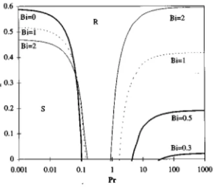
A summary of the results when the Biot and Prandtl num-bers are varied is provided in Fig. 4. This picture represents the criticalacversus the Prandtl number, for several values

of the Biot number. The region above each curve corre-sponds to stable rolls while stable square convective cells are observed under a curve. For small Pr, squares are always possible, at any value of Biot number larger than or equal to 0. Moreover, it is noticed thatacdecreases with Bi. On the

other hand, for large Prandtl numbers, the curve ac

disap-pears when Bi,0.28, which means that only rolls are stable far from the threshold in this case. In addition, it is seen that the curve ac is more sensitive to Bi for large Pr than for

small Pr. So it is necessary to know precisely the value of the FIG. 3. Stable solutions as functions ofa for Pr5100 and for different value of the Biot number. For~b! and ~c!, closeups of the e axis are provided on the right.

Biot number to determine the transition to square convection in this case. Note also that there exists a region in the neigh-borhood of Pr50.3 where squares cannot be found, whatever Bi. As a final remark about Fig. 4, let us mention that when the Biot number is increased above Bi52, the curves ac

merge into one another since a saturation effect appears. It is now interesting to compare our model with the ex-periments of Nitschke and Thess@22#. In these experiments, the Prandtl number is equal to 100 and the thickness of the fluid is equal to d51.55 mm. It is then easy to estimate precisely the value ofa. From the material properties of the fluid, it is found thata50.044. On the other hand it is well known that the Biot condition used at the top surface is an approximation introduced to avoid solving the complete con-servation equations in the gas lying above the fluid layer. In a linear analysis which takes into account the temperature perturbation in the gas, this resolution can be carried out and an accurate value for Bi can be evaluated. It is easy to show @27# that, in this context,

Bi5lgas lfl

k

tanh~kdgas!. ~21!

In this formula, lgas andlflrepresent the conductivities of the gas and the fluid; dgasis the dimensionless thickness of the gas layer, while k is the wave number. For the experi-ments of Nitschke and Thess@22#, this ‘‘linear Biot number’’ is equal to 0.44. Of course this value for Bi cannot strictly be used in the nonlinear regime for which this parameter is not clearly defined. For these reasons, we give in Fig. 5 the dif-ferent stable patterns versus the Biot number for the values of a and Pr corresponding to the experiments of Nitschke and Thess. The shaded area in this picture represents the transition to square patterns as observed experimentally. It is seen that agreement with experimental data is achieved by taking a Biot number equal to about 1.6, which is rather different from the linear value 0.44. Note finally that, a the-oretical work including a complete description of the dynam-ics of the upper gas layer was performed by Golovin et al.

@25# for pure Marangoni convection. Their predictions about the transition to square convection are also in good qualita-tive agreement with the experiments but the results are not completely satisfactory from a quantitative point of view.

V. CONCLUSION

The occurrence of square convective cells in a fluid layer heated from below ~Be´nard-Marangoni problem! has been examined. The mathematical analysis is based on Landau amplitude equations, which were deduced from the general Boussinesq equations. The main conclusions are the follow-ing. First, since only rolls are observed for largea, it is clear that the appearance of square cells is mainly due to capillary effects and therefore will be observed in thin layers. Typi-cally, squares will never be found foralarger than 0.6 ~see Fig. 4!, which corresponds to a thickness of the order of 1 cm for many fluids ~silicone oils, mercury, ethanol, glyc-erol!. It is also shown that the Biot number must be larger than 0.28 for squares to be observed in large Prandtl number fluids. When Pr is quite small, squares are possible whatever the value of the Biot number. When the Prandtl number is close to 0.3, only rolls appear. Note also that the areas where only hexagons are stable are quite smaller whena,acthan

for thicker fluid layers. It is also important to stress that qualitative agreement with the experiments of Nitschke and Thess @22# is achieved concerning the transition to square cells. However, the comparison showed the difficulty in de-fining accurately the Biot number in the nonlinear regime.

ACKNOWLEDGMENTS

This text presents research results of the Belgian Interuni-versity Poles of Attraction ~P.A.I. No. 21! initiated by the Belgian State, Prime Minister’s Office, Science Policy Pro-gramming. The scientific responsibility is assumed by its au-thors. Partial support from the European Community under Contract No. ERB-CHRX-CT94-0481 is also acknowledged. It is a pleasure to thank Professor J.-C. Legros and his group ~Brussels University! for interesting discussions.

FIG. 4. Critical value ac of parametera as a function of the Prandtl number and for different Biot numbers. Rolls or squares are stable far from the threshold for a respectively above and below each curve.

FIG. 5. Stable convective structures as functions of the Biot number for a50.044 (d51.55 mm) and Pr5100, which corre-spond to the experiments of Nitschke and Thess @22#. The shaded area defines the experimental threshold to pure square convection.

@1# A. Schlu¨ter, D. Lortz, and F. Busse, J. Fluid Mech. 23, 129 ~1965!.

@2# J. Stuart, J. Fluid Mech. 9, 353 ~1960!.

@3# L. A. Segel and J. Stuart, J. Fluid Mech. 13, 269 ~1962!. @4# L. A. Segel, J. Fluid Mech. 21, 359 ~1965!.

@5# J. Scanlon and L. A. Segel, J. Fluid Mech. 30, 149 ~1967!. @6# J. Bragard and G. Lebon, Europhys. Lett. 21, 831 ~1993!. @7# A. Cloot and G. Lebon, J. Fluid Mech. 145, 447 ~1984!. @8# P. Cerisier, C. Jamond, J. Pantaloni, and C. Pe´rez-Garcı´a,

Phys. Fluids 30, 954~1987!.

@9# J. Kraska and R. Sani, Int. J. Heat Mass Transfer 22, 535 ~1979!.

@10# S. Rosenblat, S. H. Davis, and G. M. Homsy, J. Fluid Mech. 120, 91~1982!; 120, 123 ~1982!.

@11# W. Eckhaus, Studies in Non-Linear Stability Theory ~Springer-Verlag, New York, 1965!.

@12# M. C. Cross, Phys. Fluids 23, 1727 ~1980!; Phys. Rev. A 25, 1065~1982!.

@13# P. C. Dauby, G. Lebon, P. Colinet, and J. C. Legros, Q. J. Mech. Appl. Math. 46, 683~1993!.

@14# M. Bestehorn, Phys. Rev. E 48, 3622 ~1993!.

@15# A. Thess and M. Bestehorn, Phys. Rev. E 52, 6358 ~1995!. @16# P. C. Dauby, Ph.D. thesis, University of Lie`ge, Belgium, 1994. @17# A. Thess and S. A. Orszag, J. Fluid Mech. 283, 201 ~1995!. @18# D. D. Joseph, Stability of Fluid Motions II, Springer Tracts in

Natural Philosophy Vol. 28~Springer-Verlag, Berlin, 1976!. @19# E. L. Koschmieder and S. A. Prahl, J. Fluid Mech. 215, 571

~1990!.

@20# E. L. Koschmieder and M. I. Biggerstaff, J. Fluid Mech. 167, 49~1986!.

@21# P. M. Parmentier, V. C. Regnier, G. Lebon, and J. C. Legros, Phys. Rev. E 54, 411~1996!.

@22# K. Nitschke and A. Thess, Phys. Rev. E 52, R5772 ~1995!. @23# M. Bestehorn, Phys. Rev. Lett. 76, 46 ~1996!.

@24# J. Bragard ~private communication!.

@25# A. A. Golovin, A. A. Nepomnyashchy, and L. M. Pismen ~un-published!.

@26# C. Kubstrup, H. Herrero, and C. Pe´rez-Garcı´a, Phys. Rev. E 54, 1560~1996!.