Objective and subjective assessment of perceptual factors in HDR content processing

HAL Id: hal-00861086

https://hal.archives-ouvertes.fr/hal-00861086

HAL is a multi-disciplinary open access archive for the deposit and dissemination of sci-entific research documents, whether they are pub-lished or not. The documents may come from teaching and research institutions in France or abroad, or from public or private research centers.

L’archive ouverte pluridisciplinaire HAL, est destinée au dépôt et à la diffusion de documents scientifiques de niveau recherche, publiés ou non, émanant des établissements d’enseignement et de recherche français ou étrangers, des laboratoires publics ou privés.

Objective and subjective assessment of perceptual

factors in HDR content processing

Shengnan Yan

To cite this version:

Shengnan Yan. Objective and subjective assessment of perceptual factors in HDR content processing. 2013. �hal-00861086�

I

Objective and subjective assessment of

perceptual factors in HDR content

processing

Master: MDM

Student: YAN Shengnan

Supervisors: Manish Nawaria

II

ABSTRACT

The development of the display and camera technology makes high

dynamic range (HDR) image become more and more popular. High

dynamic range image give us pleasant image which has more details that

makes high dynamic range image has good quality.

This paper shows us the some important techniques in HDR images. And it

also presents the work the author did.

The paper is formed of three parts.

The first part is an introduction of HDR image. From this part we can know

why HDR image has good quality.

The second part is about the related work. It introduces some important

techniques in HDR images. From this part we can know how to acquire a

HDR image, how to encode HDR images, how to compress HDR images

and how to model human’s response to HDR images. It also shows us the

tone mapping techniques which is used in display HDR image on LDR

display.

The third part is about the research work did by myself. It is formed by two

parts, one is about the optimizing of the pooling function in HDR-VDP-2

and the other is Compare the impact of TM in HDRI compression.

III

1.Introduction of HDR images 1

2 Related Work 2

2.1 Acquisition of HDR images 2

2.2 Encodings of HDR images 3

2.2.1 Radiance RGBE Encoding (HDR) 3

2.2.2 ILM OpenEXR (EXR) 4

2.2.3 SGI LogLuv (TIFF) 4

2.3 Display of HDR image: Tone mapping 5

2.3.1 Global tone mapping 5

Global tone mapping based on linear algorithm 5

Global tone mapping based on gamma algorithm 6

Global tone mapping based on logarithmic mapping 7

Global tone mapping based on histogram equalization 8

2.3.2 Local tone mapping 9

Local tone mapping based on a decomposition of the image 9

Local tone mapping based on gradients of images 10

Local tone mapping based on Photographic 12

Local tone mapping based on iCAM 14

2.3.3 Inverse Tone mapping 16

2.4 HDR image compression using optimized TM model 17

2.5 The Visual difference predictor 18

2.5.1 Optical and retinal pathway 19

2.5.2 Multi-scale decomposition 22

2.5.3 Neural noise 22

2.5.4 Visibility metric 24

3 Research Work 26

3.1 optimize the pooling function of HDR-VDP-2 26

3.1.1 Reason for research 26

3.1.2 Implement 28

3.1.3 Results and Conclusion 29

3.2 Compare the impact of TM in HDRI compression 30

3.2.1 reason for reasch 30

3.2.2 Implement 31

3.1.3 Results and Conclusion 31

1

1. Introduction of HDR images

Dynamic range is a ratio of the highest and the lowest luminance in an image. As we all known, the dynamic range of the real world is much bigger than the pictures that we can capture by the equipment such as cameras. For example, a scene showing both shadows and sunlit areas will have a dynamic range exceeding 100,000:1. We can show many of these kinds of examples. For instances, human visual system is capable of perceiving light intensities over a range of 4 orders of magnitude. However, conventional monitors and other reproduction media such as printing papers have limited dynamic ranges. They often have a dynamic range less than 2 orders of magnitude. That means lots of information of the real world will be lost when we see the same scene in monitors or printing papers. High dynamic range images are developed to solve these problems. With the development of the technologies for increasing the dynamic range of image, high dynamic range images become more popular. It is expected to be widely used in digital cinema, digital photography and next generation broadcast, because of its high quality and its powerful expression ability. HDR imaging technologies have great influence in imaging industry. That is because HDR imaging technologies not only has high accuracy that matches the processing of the human eye but also contains enough information to achieve the desired appearance of the scene on a variety of output devices.

Figure 1.1 Example of an imaging pipeline.

Figure 1 shows an example of the way to process a HDR image, as we can see, it starts with the acquisition of a real world scene or rendering of an abstract model using computer graphics techniques and ends at a display. Here we can talk about the process of HDR images based on figure 1. Firstly, we need to know how to get the HDR images, is it the same way as we get the LDR images? After getting the HDR images we need to storage it. The encoding methods of HDR images are different from the LDR images. Most of the display devices are belong to low dynamic range, they can not display the HDR images well. To display the HDR images, different kinds of tone mapping operator which can compress the dynamic range are needed. And then, to transmit the HDR images we need to compress them, and the compression of HDR images is also different from the HDR images. When we see the HDR images our perception of the images is different, so quality assessment is very import. All of the five aspects are important for HDR image processing.

2

2 Related Work

2.1 Acquisition of HDR images

There are two ways to acquire HDR images.

The first method to acquire the HDR images is to use the devices that can capture high dynamic range data. Image capturing and display technologies have improved to span the wider dynamic range and true color representations in the last decade. They are used in various fields such as radiometry, seismology, etc. There are already devices on the market that are natively designed to capture HDR images. So we can acquire the HDR images directly by the HDR devices.

On the other hand, most of the monitors and cameras are low dynamic range. So we need to find a way to use the LDR devices to get the HDR images. The second method to acquire HDR images is called multi-exposure technique. Several methods have been proposed to improve the dynamic range of general photographs based on a multiple exposure principle. The main four steps are as follow. Firstly, photographs of still objects are taken off line by a camera at a fixed location. Secondly, a camera response curve is estimated from the multiple exposures set by self-calibration. Thirdly, linearize the images by applying the inverse of the response curve, and finally, merge the linearized images. These four steps is a basic procedure for the HDR acquisition and many of conventional algorithms follow it. This method can not only increase the dynamic range but also reduce the noise in an image. But the values of luminance can be distorted by camera optics. When increase the exposure time low-light details can be seen clearly but high-light details are lost. On the other hand, when decrease exposure time high-light details can be seen clearly. The sequence of photographs is then merged to create an HDR image which contains the values of luminance proportional to the real scene.

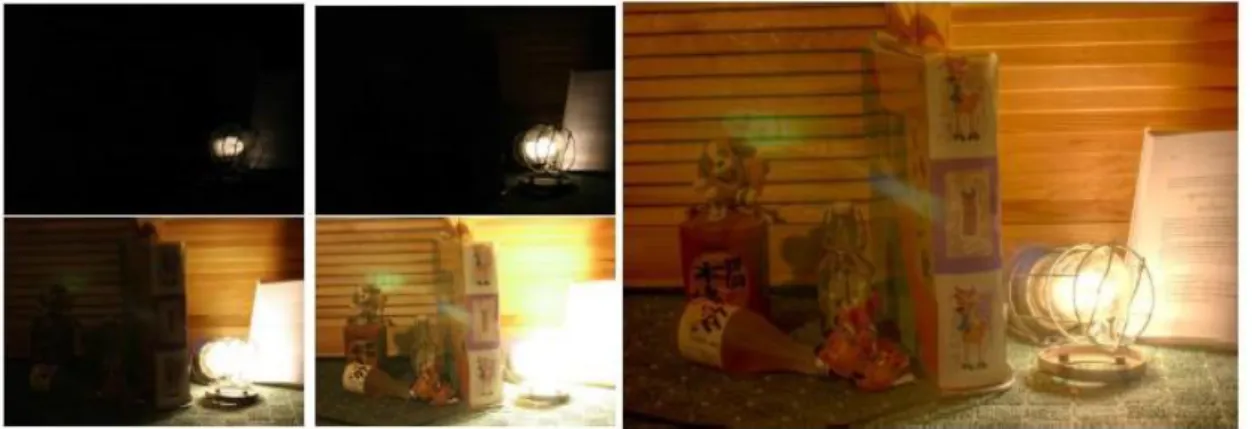
Figure 2.1 Example of multi-exposure technique

Figure 2.1 shows the way we use the multi-exposure technique to get the HDR image. We can see the final HDR image can not only show the details of low luminance but also the details of high luminance part. The multi-exposures technique can be easily

3

used but it still has a disadvantage. It is assumed that a scene is completely still during taking photographs. Therefore if there is any motion of objects or camera shake, ghosting artifacts will appear after combining the images.

2.2 Encodings of HDR images

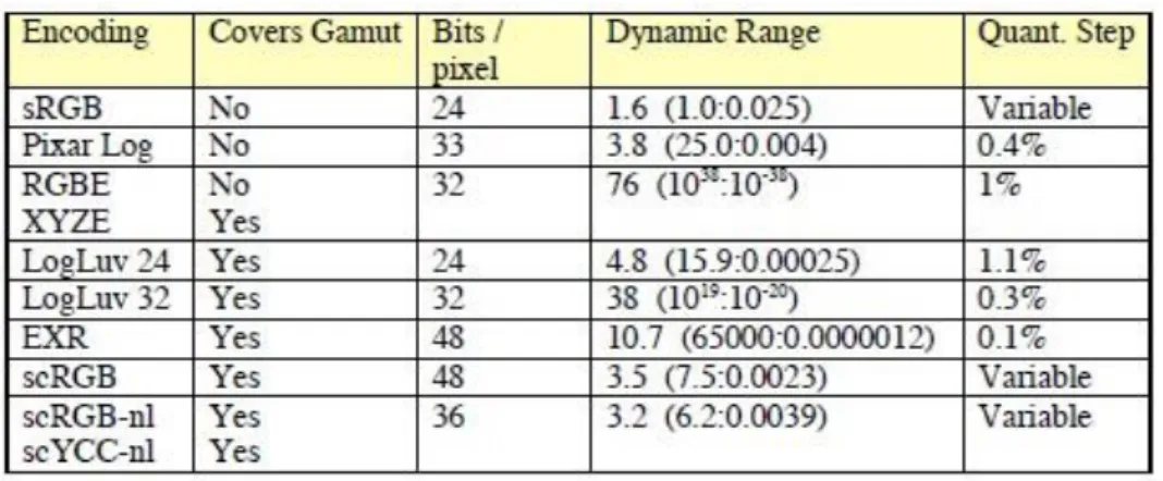
We stand on the threshold of a new era in digital imaging. Image files will encode the color gamut and dynamic range of the original scene, rather than the limited subspace that can be displayed with conventional monitor technology. In order to accomplish this goal, we need to agree upon a standard encoding for high dynamic range (HDR) image information. There are many HDR standards as shown in figure 2.2.

Figure 2.2 HDR encoding standards

As we can see, most of the standards are pixel encodings that extend over 4 orders of magnitudes, and they also can encompass the visible color gamut. They have a luminance step size below 1% and good color resolution, they will be able to encode any image with fidelity as close to perfect as human vision is capable of discerning. Here we will introduce 3 of them.

2.2.1 Radiance RGBE Encoding (HDR)

The Radiance RGBE format uses one byte for the red mantissa, one for the green, one for the blue, and one for a common exponent. The exponent is used as a scaling factor on the three linear mantissas. The largest of the three components will have a mantissa value between 128 and 255, and the other two mantissas may be anywhere in the 0-255 range. The net result is a format that has an absolute accuracy of about 1%, covering a range of over 76 orders of magnitude.

Although RGBE is a big improvement over the standard RGB encoding, both in terms of precision and in terms of dynamic range, it has some important shortcomings. Firstly, the dynamic range is much more than anyone else could ever utilize as a color representation. The sun is about 108cd/m2, and the underside of a rock on a moonless night is probably around 10-6, leaving about 62 orders of useless magnitude. It would have been much better if the format had less range but better precision in the same number of bits. This would require abandoning the byte-wise format for something like a log encoding. Another problem is that any RGB representation restricted to a positive

4

range, such as RGBE and Pixar’s Log format, cannot cover the visible gamut using any set of “real” primaries. Finally, the distribution of error is not perceptually uniform with this encoding.

2.2.2 ILM OpenEXR (EXR)

This format is a general-purpose wrapper for the 16-bit half data type. It has also been called the “S5E10” format for “Sign plus 5 exponent plus 10 mantissa,” and this format has been floating around the computer graphics hardware developer network for some time. Because it can represent negative primary values along with positive ones, the OpenEXR format covers the entire visible gamut and a range of about 10.7 orders of magnitude with a relative precision of 0.1%. Since humans can simultaneously see no more than 4 orders of magnitude, this makes OpenEXR a good candidate for archival image storage.

Although the basic encoding is 48 bits/pixel as opposed to 32 for the LogLuv and RGBE formats, the additional precision is valuable when applying multiple blends and other operations where errors might accumulate. It would be nice if the encoding covered a larger dynamic range, but 10.7 orders is adequate for most purposes, so long as the exposure is not too extreme. The OpenEXR specification offers the additional benefit of extra channels, which may be used for alpha, depth, or spectral sampling. This sort of flexibility is critical for high-end compositing pipelines, and would have to be supported by some non-standard use of layers in a TIFF image.

The OpenEXR format has clear advantages for high quality image processing, and is supported directly by today’s high-end graphics cards.

2.2.3 SGI LogLuv (TIFF)

The SGI LogLuv format is based on visual perception. It separates the luminance and chrominance channels, and applying a log encoding to luminance. That makes the quantization steps match human contrast and color detection thresholds. There are actually three variants of this logarithmic encoding. The first pairs a 10-bit log luminance value together with a 14-bit CIE (u´,v´) lookup to squeeze everything into a standard-length 24-bit pixel. This was mainly done to prove a point, which is that following a perceptual model allows you to make much better use of the same number of bits. In this case, we were able to extend to the full visible gamut and 4.8 orders of magnitude of luminance in just imperceptible steps. The second variation uses 16 bits for a pure luminance encoding, allowing negative values and covering a dynamic range of 38 orders of magnitude in 0.3% steps, which are comfortably below the perceptible level. The third variation uses the same 16 bits for signed luminance, then adds 8 bits each for CIE u´ and v´ coordinates to encompass all the visible colors in 32 bits/pixel. It uses 10-bit for log luminance value and a 14-bit for CIE (u´,v´).

It aims at improving the RGBE to provide a standard for HDR image encoding. It works extremely well for HDR image encoding, appropriate format for the archival storage of color images. But a simple 3*3 matrix for the translation from RGB to CIE is needed. People’s reluctance to deviate from their familiar RGB color space maybe is one of the reason why we do not found the widespread use of it.

5

2.3 Display of HDR image: Tone mapping

Although we have HDR devices to capture or display HDR images, most of the display devices are low dynamic range. So when we display HDR images on conventional reproduction media such as LCD panels, it will cause significant limitations in image analysis, processing and displaying of data. One way to solve this problem is to compress the high dynamic range to low dynamic range which is fit into the dynamic range of the display devices. This technology is called tone mapping. It is introduced in the graphic pipeline as the last step before image display. With tone mapping we can present images similar to the original scenes to human viewers although the displaying hardware has physical limitations. Tone mapping should provide drastic contrast reduction from scene values to displayable ranges while preserving the image details. In recent years several tone mapping methods have been developed. We can classify these methods into two broad categories, the global tone mapping and the local tone mapping. The global tone mapping technology uses a single invariant tone mapping function for all pixels in the image, but the local tone mapping technology uses different tone mapping functions for different pixels in the image. The local tone mapping technology adapts the mapping functions to local pixel statistics and local pixel contexts. Global tone mapping is simpler to implement but is easier to lose details. Local tone mapping can save details but it is difficult in computation.

In this section we will have a specific introduction of some tone mapping algorithms.

2.3.1 Global tone mapping

Global tone mapping is conceptually simple, computationally efficient, robust, and easy to use. Here we will show some of the typical global tone mapping functions which is widely used.

Global tone mapping based on linear algorithm

We can give an example to show how the global tone mapping filter works. ………..(2.1)

Vin is the luminance of the original pixel and Vout is the luminance of the output pixel.

We can see this function can map the luminance Vin in the domain [0, ∞) to a output

range of [0,1). But we can also see it has obviously disadvantage, parts of the image with higher luminance will get increasingly lower contrast as the low luminance parts of.

We can show another example of linear tone mapping. The linear tone mapping function I use in matlab for test is imgOut=((y)./(p*max(max(max(y))))); Here y is the input image, p is a parameters we can set freely. And the output image is figure 2.3.

6 Figure 2.3 an example of linear tone mapping.

The right one is the original image and the left one is the new image after tone mapping, we can see some details in the LDR image of the dark place that can not be seen in the original image. But we can also see some details are lost. So although linear tone mapping is easy to use, it does not work very well sometimes it has lots of disadvantages.

Global tone mapping based on gamma algorithm

A perhaps more useful global tone mapping method is gamma compression. To improve contrast in dark areas, changes to the gamma correction procedure are proposed. This adaptive logarithmic mapping technique is capable of producing perceptually tuned images with high dynamic content and works at interactive speed. The filter is as follow,

Vout = AVin

γ_{………..(2.2)}

where A > 0 and 0 < γ < 1. This function will map the luminance Vin in the domain

[0,1/A1/γ] to the output range [0,1], γ regulates the contrast of the image, a lower value for lower contrast. While a lower constant γ gives a lower contrast and perhaps also a duller image, it increases the exposure of underexposed parts of the image while at the same time, if A < 1, it can decrease the exposure of overexposed parts of the image enough to prevent them from being overexposed. Ward global tone mapping is one of gamma tone mapping. The tone mapped image is figure 2.4.

Figure 2.4 an example of gamma tone mapping

The right one is the original image and the left one is the new image after tone mapping, we can see more details of the dark place in this LDR image than the LDR image get

7

from linear tone mapping. But we can also see some details are lost.

Global tone mapping based on logarithmic mapping

To improve the linear tone mapping, lots of methods for tone mapping are developed. One is the logarithmic tone mapping which is based on the Weber-Fechner law. Weber-Fechner law shows that our human eyes response to luminance is similar as the logarithmic. We can use logarithmic to compress the luminance values, so that we can imitate the human response to light. The response of the human visual system to stimulus luminance L can be described as follow,

B = k1 ln(L/L0)………..(2.3)

Here L0 is the background luminance and k1 is a constant. We can see human visual

system has a linear relationship of the logarithmic of the ratio of luminance. The most popular used function is recommended by Stockham4.

………..(2.4)

where Ld is displayed luminance , Lw is world luminance, and Lmax is maximum

luminance in the scene. This tone mapping function ensures that whatever the dynamic range of the scene is, the maximum value is remapped to one and other luminance values are smoothly incremented. An example of logarithm tone mapping is shown in figure 2.5.

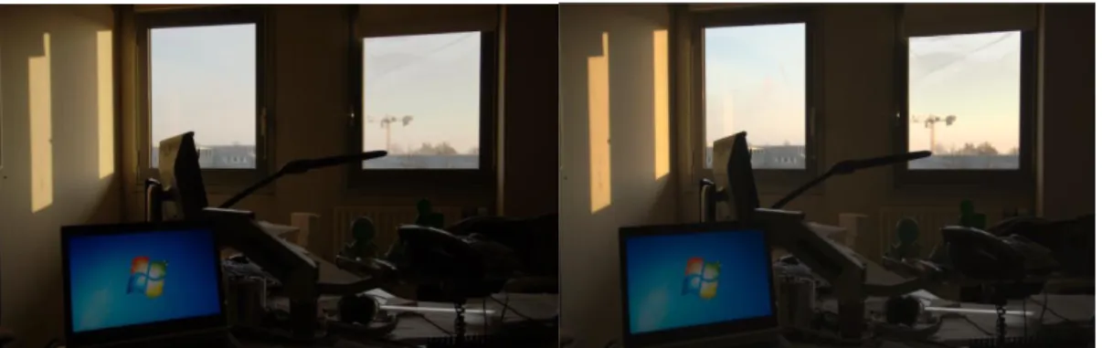
Figure 2.5 an example of logarithm tone mapping

The right one is the original image and the left one is the new image after tone mapping, we can see lots of details not only in the dark places but also in the very bright parts. We can see this method is much better than the linear tone mapping and gamma tone mapping.

While this formula leads to pleasant images, we found that the luminance compression is excessive and the feeling of high contrast content is lost5. When use the logarithm to adjust the contrast, the most important thing is to adjust the logarithmic bases. Different logarithmic bases will cause different result. To solve these problems, a bias power function is introduced to adaptively vary logarithmic bases in one paper[5] by Drago. The results of the preservation of details and contrast are really good. The new logarithmic mapping is as follow,

8

…………..(2.5)

Ld is a displaying value and Lw is luminance value. Lwmax is the value of Lw multiply the

exposure value which can be changed by the user. Ldmax is the maximum luminance

capability of the displaying medium. It is used as a scale factor to adapt the output to its intended display. We can use a value for Ldmax = 100 cd/m2, a common reference value

for CRT displays. The bias parameter b is essential to adjust compression of high values and visibility of details in dark areas. The value of b in the range of [0.5,1] can get better results. The tone mapped image is figure 2.6.

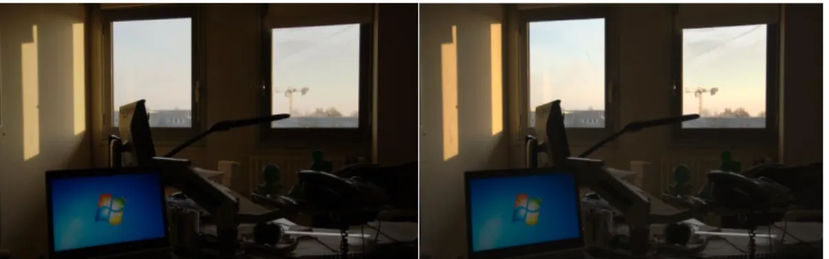
Figure 2.6 another example of logarithm tone mapping

The right one is the original image and the left one is the new image after tone mapping. We can see this method get pleasant images. We can see some high contrast content.

Global tone mapping based on histogram equalization

Histogram equalization is also widely used in tone mapping technology. These methods seek to adjust the image to make it easier to analyze or improve visual quality. This method usually increases the global contrast of many images, especially when the usable data of the image is represented by close contrast values. This allows for areas of lower local contrast to gain a higher contrast. Histogram equalization accomplishes this by effectively spreading out the most frequent intensity values. The base function of histogram equalization is as follow,

………(2.6)

Here v is the value of original pixel, L is the grey levels, M × N is the image's number of pixels and cdf is the cumulative distribution function. We can compress the dynamic range by this function. We can see the compression result is as follow.

9

X axis is the value of the pixels, and y axis is the accumulated of the pixels that has the same values.

2.3.2 Local tone mapping

Local tone mapping operators use a mapping that varies spatially depending on the neighborhood of a pixel. This is based on the fact that human vision is sensitive mainly to local contrast. Most local tone-mapping techniques use a decomposition of the image into different layers or scales. The contrast is reduced differently for each scale, and the final image is a recomposition of the various scales after contrast reduction. Here we show some of the tone mapping functions.

Local tone mapping based on a decomposition of the image

When we use the tone mapping functions we want to reduce the contrast and preserve details. So we can decompose the image into two different layers, a base layer and a detail layer. This decomposition is motivated by two widely accepted assumptions in human vision. Firstly, human vision is mostly sensitive to the details of an image rather than the illumination conditions. Secondly, human vision is mostly sensitive to local contrast rather than the global contrast.

I(x,y) =B(x,y)＋D(x,y)………..(2.7)

I(x,y) is the original image, B(x,y) is the base layer of the original image and D(x,y) is the detail layer of the original image.

The base layer is obtained using an edge-preserving filter called the bilateral filter. It is a non-linear filter where the output is a weighted average of the input. The weight of each pixel is computed using a Gaussian in the spatial domain multiplied by an influence function in the intensity domain that decreases the weight of pixels with large intensity differences. The detail layer is achieved by subtracting the base layer image from the original image.

The fact that the human visual system is insensitive to the global luminance contrast enables the solution of compressing the global dynamic range and preserving local details in an HDR scene to reproduce the same perceptual appearance on a LDR display. The components of base layer change slowly but detail layer do not. So we can use one tone mapping function to compress the dynamic range of the base layer but do not compress the detail layer.

I2(x,y) =B2(x,y)＋D(x,y)……….(2.8)

Only the base layer has its contrast reduced, thereby preserving details. The method is fast, stable, and requires no setting of parameters. We can get good results from this method, but we still have a problem of haloing which shows a dark curve around the very bright part of the image. The major disadvantage of local methods is the presence of haloing artifacts. When dealing with high-dynamic-range images, haloing issues become even more critical. Many papers are written to solve this problem. One popular used way is introduced by Durand. In this method, the pixel value divided by adjacent pixels which have similar pixel values. We can accelerate bilateral filtering by using a piecewise-linear approximation in the intensity domain and appropriate subsampling.

10

This results in a speed-up of two orders of magnitude. The method is fast and requires no parameter set[6]. We can see the compression result is as follow.

Figure 2.8 an example of Local tone mapping based on a decomposition of the image

The right one is the original image and the left one is the new image after tone mapping. We can see this method get pleasant images. But computing such a separation for real images is an ill posed problem.

Local tone mapping based on gradients of images

This approach relies on the widely accepted assumptions that the human visual system is not very sensitive to absolute luminance, but rather sensitive to local intensity ratio changes. This algorithm is also based on the rather simple observation that drastic change in the luminance across a high dynamic range image can cause large magnitude luminance gradients. Fine details, on the other hand, can cause gradients of much smaller magnitude. The idea is then to identify large gradients at various scales, and compress their magnitudes while keeping their direction unchanged. The compression to larger gradients must be more heavily than to smaller ones. So we can compress drastic luminance changes, while preserving fine details. A reduced high dynamic range image is then reconstructed from the compressed gradient field. It should be noted that all of the computations are done on the logarithm of the luminance, rather than on the luminance themselves. That is because the logarithm of the luminance is an approximation to the human perceived brightness, and gradients in the log domain correspond to ratios in the luminance domain. We can have a look of an example of a high dynamic range 1D function.

Figure 2.9 an example of tone mapping based on gradients of images 1D function

The picture (a) shows an input HDR scanline with dynamic range of 2415:1. Picture (b) shows the results of a logarithm used after the scanline, H(x) equals to log(scanline). Picture (c) is the derivatives of H(x). Picture (d) is the attenuated derivatives G(x), and picture (e) is the reconstructed signal I(x). Picture (f) is an LDR scanline of exponent of I(x) and the new dynamic range is 7.5:1. We must note that each plot uses a different

11

scale for its vertical axis in order to show details, except (c) and (d) that use the same vertical axis scaling in order to show the amount of attenuation applied on the derivatives.

For the 2D images we can compress the dynamic range as follow. Firstly, We begin by constructing a Gaussian pyramid H0,H1,…,Hd, where H0 is the full resolution HDR

image and Hd is the coarsest level in the pyramid. d is chosen such that the width and

the height of Hd are at least 32. At each level k we compute the gradients using central

differences:

……….(2.9)

At each level k a scaling factor ϕk(x, y) is determined for each pixel based on the

magnitude of the gradient there:

………(2.10)

The first parameter α determines which gradient magnitudes remain unchanged. Gradients of larger magnitude are attenuated (assuming β < 1), while gradients of magnitude smaller than α are slightly magnified. In all the results shown in this paper we set α to 0.1 times the average gradient magnitude, and β between 0.8 and 0.9. The full resolution gradient attenuation function Φ(x, y) is computed in a top-down fashion, by propagating the scaling factors ϕk(x, y) from each level to the next using

linear interpolation and accumulating them using point wise multiplication. More formally, the process is given by the equations:

……….…(2.11)

where d is the coarsest level, Φk denotes the accumulated attenuation function at level

k, and L is an up sampling operator with linear interpolation.

After these two steps we can get a compressed gradient map, and we can use this map to get the LDR image. We suppose the LDR image to be I, the compressed gradient map to be G. I and G has the relationship as follow,

∇2

I(x, y) = divG ………(2.12)

Since both the Laplacian ∇2

and div are linear operators, approximating them using standard finite differences yields a linear system of equations. More specifically, we can approximate:

∇2

I(x, y)≈I(x+1, y)+I(x−1, y)+I(x, y+1)+I(x, y−1)−4I(x, y)……….(2.13)

The gradient ∇H is approximated using the forward difference

∇H(x, y) ≈ (H(x+1, y)−H(x, y),H(x, y+1)−H(x, y)) ………...…(2.14) while for divG we use backward difference approximations

12

So from the 4 functions above, finally we can get I.

This method is conceptually simple, computationally efficient, robust, and easy to use. We manipulate the gradient field of the luminance image by attenuating the magnitudes of large gradients. A new, low dynamic range image is then obtained by solving a Poisson equation on the modified gradient field. And the results demonstrate that the method is capable of drastic dynamic range compression, while preserving fine details and avoiding common artifacts, such as halos, gradient reversals, or loss of local contrast. The method is also able to significantly enhance ordinary images by bringing out detail in dark regions[9]. We can see the compression result is as follow.

Figure 2.10 an example of Local tone mapping based on gradients of the image

The right one is the original image and the left one is the new image after tone mapping. We can see this method get pleasant images.

Local tone mapping based on Photographic

Photographers aim to compress the dynamic range of a scene to create a pleasing image. Some algorithms borrow from 150 years of photographic experience. A classic photographic task is the mapping of the potentially high dynamic range of real world luminance to the low dynamic range of the photographic print. This tone reproduction problem is also faced by computer graphics practitioners who map digital images to a low dynamic range print or screen. The resulting algorithm is simple and produces good results for a wide variety of images.

Firstly, we need to get the log-average luminance as a useful approximation to the key of the scene.

………...……(2.16)

where Lw(x, y) is the “world” luminance for pixel (x, y), N is the total number of pixels

in the image and δ is a small value to avoid the singularity that occurs if black pixels are present in the image. And then, we can use a function as follow to compress the dynamic range.

………...……(2.17)

where Lwhite is the smallest luminance that will be mapped to pure white. For many high

13

sufficient to preserve detail in low contrast areas, while compressing high luminances to a displayable range. However, for very high dynamic range images important detail is still lost. For these images a local tone reproduction algorithm that applies dodging-andburning is needed[10].

In traditional dodging-and-burning, all portions of the print potentially receive a different exposure time from the negative, bringing “up” selected dark regions or bringing “down” selected light regions to avoid loss of detail. With digital images we have the potential to extend this idea to deal with very high dynamic range images. We can think of this as choosing a key value for every pixel. Dodging-and-burning is typically applied over an entire region bounded by large contrasts. The size of a local region is estimated using a measure of local contrast, which is computed at multiple spatial scales. Such contrast measures frequently use a center-surround function at each spatial scale, often implemented by subtracting two Gaussian blurred images. A center-surround function derived from Blommaert’s model for brightness perception is used here. This function is constructed using circularly symmetric Gaussian profiles of the form:

………...(2.18)

These profiles operate at different scales s and at different image positions (x, y). Analyzing an image using such profiles amounts to convolving the image with these Gaussians, resulting in a response Vi as function of image location, scale and

luminance distribution L:

Vi(x, y, s) = L(x, y) ⊗ Ri(x, y, s) ………...……(2.19)

This convolution can be computed directly in the spatial domain, or for improved efficiency can be evaluated by multiplication in the Fourier domain. The smallest Gaussian profile will be only slightly larger than one pixel and therefore the accuracy with which the above equation is evaluated, is important. We perform the integration in terms of the error function to gain a high enough accuracy without having to resort to super-sampling. The center-surround function we use is defined by:

………...(2.20)

where center V1 and surround V2 responses are derived from the two upper equations.

This constitutes a standard difference of Gaussians approach. The free parameters a and φ are the key value and a sharpening parameter respectively.

Equation 4.20 is computed for the sole purpose of establishing a measure of locality for each pixel, which amounts to finding a scale sm of appropriate size. The area to be

considered local is in principle the largest area around a given pixel where no large contrast changes occur. To choose the largest neighborhood around a pixel with fairly even luminances, we threshold V to select the corresponding scale sm. Starting at the

lowest scale, we seek the first scale sm :

14

Here e is the threshold. So we can observe that V1(x, y, sm) may serve as a local average

for that pixel. The global tone reproduction operator can be converted into a local operator by replacing L with V1 in the denominator:

………...……(2.22)

Here is an example of local tone mapping based on photographic of Reinhard TMO.

Figure 2.11 an example of Local tone mapping based on Photographic

The right one is the original image and the left one is the new image after tone mapping. We can see all the details of dark places clearly.

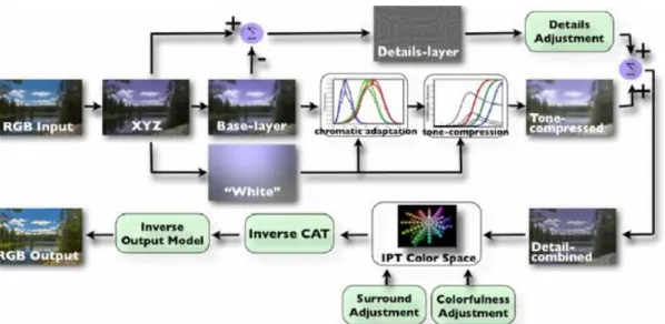
Local tone mapping based on iCAM

Image appearance models extend color appearance models to incorporate properties of spatial and temporal vision allowing prediction of the appearance of complex stimuli. Given an input of images and viewing conditions, an image appearance model can provide perceptual attributes of each pixel, not only limited to the traditional color appearance correlates such as lightness, but rather those image attributes such as contrast and sharpness. Spatial color appearance models, were first proposed by incorporating spatial filtering to measure the difference between two images, extending the application of traditional color difference equations in measuring the perceptual difference between complex stimuli. The filtering computation is dependent on viewing distance and is generally derived from human contrast sensitivity functions. More recent results suggest that while such multi-scale filtering might be critical for some threshold metrics, it is often not necessary for supra-threshold predictions of image attributes and perceived image differences. Image color appearance model (iCAM)[8] was proposed to preserve simplicity and ease of use by adopting a single-scale spatial filtering.

As image appearance models attempt to predict the perceptual response towards spatial complex stimuli, they can provide a unique framework for the prediction of the appearance of HDR images. Without changing its general framework, iCAM has been extended into the application of HDR image rendering. Recent tone-mapping operator evaluation results showed that iCAM is effective in HDR image rendering, however, iCAM does not perform as well as some of other operators, such as the bilateral filter. The next generation of image appearance model, designated iCAM06, was developed for HDR image rendering application. Several modules have been inherited from the

15

iCAM framework, such as the local white point adaptation, chromatic adaptation, and the IPT uniform color space. A number of improvements have been implemented in iCAM06 on the motivation of a better algorithm that is capable of providing more pleasing and more accurate HDR renderings, and even a more developed perceptual model for a wider range of image appearance prediction.

Figure 2.12 an explain of histogram equalization

Firstly, when we get the RGB input image we can transform it into CIE tristimulus values (XYZ). The absolute luminance Y of the image data is necessary to predict various luminance-dependent phenomena, such as the Hunt effect and the Stevens effect. And then, we can use the bilateral filter to decompose the image into a base layer and a detail layer.

Secondly, the modules of chromatic adaptation and tone-compression processing are applied to the base layer. The base layer image is first processed through the chromatic adaptation.

………...……(2.23)

The incomplete adaptation factor D is computed as a function of adaptation luminance LA and surround factor F (F = 1 in an average surround).

The post-adaptation nonlinear compression is a simulation of the photoreceptor responses, including cones and rods. Therefore, the tone compression output in iCAM06 is a combination of cone response and rod response. The CIECAM02 post-adaptation model is adopted as cone response prediction in iCAM06 since it was well researched and established to have good prediction of all available visual data. The chromatic adapted RGB responses are first converted from the CAT02 space to Hunt-Pointer-Estevez fundamentals using the CIECAM02 formula. After that we can use the tone mapping function as follow,

16

………...……(2.24)

The color channel G and B is compressed similar as R. However, the computation of the FL factor in iCAM06 is quite different from that in the previous color appearance

models, as it is derived from the low-pass adaptation image at each pixel location and thus spatially varied in iCAM06. Yw is the luminance of the local adapted white

image. A filter size of 1/3 the shorter dimension of the image size works well for our experimental images, though again it should be stressed that this is based on an assumption for the viewing conditions. For unusually large or small images this parameter might need to be altered. The rod response after adaptation, As, is given as follow,

………...……(2.25)

Here, s is the luminance of each pixel in the chromatic adapted image, and Sw is the

value of S for the reference white. By setting Sw to a global scale from the maximum

value of the local adapted white point image, the rod response output is automatically adjusted by the general luminance perception of the scene. LAS is the dark luminance,

BS is the rod pigment bleach or saturation factor, and FLS is the dark luminance level

adaptation factor. The final tone compression response is a sum of the cone response and the rod response, given as follow,

RGBTC = RGB’+AS………...……(2.26)

The rod response after adaptation, As Evaluation of the model proved iCAM06 to have consistently good HDR rendering performance in both preference and accuracy.

2.3.3 Inverse Tone mapping

Tone mapping operators compress the luminance range while trying to maintain contrast. The inverse of tone mapping, inverse tone mapping, expands a low dynamic range image into an HDR image. HDR images contain a broader range of physical values that can be perceived by the human visual system. But the majority of today’s media is stored in the low dynamic range. Inverse tone mapping operators (iTMOs) could thus potentially revive all of this content for use in high dynamic range display. Many new frameworks were introduced to find a solution to this problem. Most of them is based on the original tone mapping methods.They try to use the inverse operation of the original operator to mapping the LDR images to HDR images. Some of them also set frameworks to make the inverse tone mapping gain more details of the images. One

17

widely used example uses importance sampling of light sources to find the areas considered to be of high luminance and subsequently applies density estimation to generate an expand map in order to extend the range in the high luminance areas using an inverse tone mapping operator.

2.4 HDR image compression using optimized TM model

The paper[16] gives us a coding algorithm for HDR images. Their encoder applies a tone mapping model based on scaled μ-Law encoding, followed by a conventional LDR image (LDRI) encoder. The tone mapping model is designed to minimize the difference between the tone mapped HDR image and its LDR version. Use this method not only the quality of the HDRI but also the one of LDRI is improved. The outline of the encoder is in Fig.2.13(a), and the outline of the decoder is in Fig.2.13(b).

Fig.2.13 outline of the encoder(a) and decoder(b)

where ‘TM’ is a tone mapping operator and f() is an approximated model for the TM, and Q is quantization. Given a HDR image, we first convert it to a LDR image by a user-selected tone mapping operator. Any operator can be used unless it intends to yield unnatural effects. Using the two images, the HDR image and its tone mapped LDR image, the parameters of our tone mapping model are found by nonlinear least squares optimization. Then the HDR image is transformed by the tone mapping model with the optimized parameters, followed by the quantization. Finally the transformed image is input to JPEG2000. The decoder, illustrated in Fig.2.13(b), applies its inverse tone mapping model f-1() after the JPEG2000 decoding. The parameters of the tone mapping model are sent to the decoder as side information.

The most effective way to evaluate the visual quality is based on the Human Visual System (HVS). Especially a nonlinear relationship to luminance is important for the HDRI compression. It is widely agreed that there is a nonlinear relationship between an amount of sensation and intensity of lights. So we can choose Weber-Fechner’s Law our method optimizes a tone mapping operator to minimize the error between the HDRI and the LDRI converted by a particular tone mapping operator. The tone mapping model is as follow,

18

………...……(2.27)

where s is a scaling parameter and μ is a parameter to control the depthof logarithm. Its inverse function is given by

…….………..(2.28)

We choose this function due to some desirable properties: Firstly, the function is controlled only by two parameters. Secondly, the function is invertible. To design the model, we first select a tone mapping operator that will be actually used after decoding. Then the LDR image is created by the operator. We find the parameter s and μby minimizing a cost function:

………...……(2.29)

where, H and L are the HDR image and its tone mapped LDR image, and the suffix i is a pixel index.

In this method, the intensity of an input color image is calculated, and then the optimization is done for the intensity. Each of RGB channels is transformed by the same optimized model. After the image is transformed, it is uniformly quantized to integer in order to input the JPEG2000 encoder, that is,

………...…………..…(2.30)

where y is an input to the JPEG2000 encoder and H is the quantization operator. Since the HDR images are used after tone mapping in many applications, improving the quality of LDR images is important. Our technique uses the tone mapping model that is optimized to minimize the error between the HDR images and its tone mapped version for pre-processing before JPEG2000 compression. This method is better than the conventional method in senses both of the HDR images and LDR images.

This technique uses the tone mapping model that is optimized to minimize the error between the HDR images and its tone mapped version for pre-processing before JPEG2000 compression. This method is better than the conventional method in senses both of the HDR images and LDR images.

2.5 The Visual difference predictor

The visible differences predictor (VDP) is an algorithm for describing the human visual response. It is the visible differences predictor which use an algorithm for the assessment of image fidelity. Unfortunately, the VDP of Daly model works well for narrow intensity ranges, and do not correlate well with experimental data outside these ranges. Handling a wide range of luminance is essential for the new high dynamic range display technologies or physical rendering techniques, where the range of luminance can vary greatly. To address these issues, we need a visual metric for predicting visibility and quality. The new metric named HDR-VDP-2 is widely used and it is

19

based on a new visual model for all luminance conditions, which has been derived from new contrast sensitivity measurements.

To get the visibility and quality predictions for HDR images, we need to mimic the visual system. When mimic the visual system, we have to deal with different aspects. Firstly, we need an accurate fit to the experimental data. Secondly, we want to make the computation not too complex. Thirdly, we want to get a model of actual biological mechanisms. The former one is the most important one. So based on this three roles, HDR-VDP-2 is created. The overall architecture of the proposed metric which mimics the visual system is shown as follow, and the diagram also summarizes the symbols used throughout the paper. In this part we want to show how it works.

Figure 2.14 The visual difference predictor

We can see the inputs are a test image and a reference image. Usually a test image contains a feature that is to be detected but a reference image lacks. For example, for measuring compression distortions the pair can be an image before and after compression. Since the visual performance differs dramatically across the luminance range as well as the spectral range, the input to the visual model needs to precisely describe the light falling onto the retina. Both the test and reference images are represented as a set of spectral radiance maps, where each map has associated spectral emission curve. This could be the emission of the display that is being tested and the linearized values of primaries for that display. The following sections are organized to follow the processing flow shown in next figure, with the headings that correspond to the processing blocks.

2.5.1 Optical and retinal pathway

Optical and retinal pathway starts from the eyes get the scene spectral radiance maps, then it model the light scatter in human eyes, the human visual system response to the light and human visual system pay different sensitivity of different luminance intensity. Figure 3.3 shows how optical and retinal pathway, in this part we will introduce them in detail.

20 Figure 2.14 Optical and retinal pathway of the HDR-VDP-2

Intra-ocular light scatter. A small portion of the light that travels through the eye is

scattered in the cornea, lens, inside the eye chamber and on the retina. Such scattering can compress the high spatial frequencies, but more importantly, it causes a light pollution. The pollution can reduce the contrast of the light projected on the retina. The effect is especially pronounced when observing scenes of high contrast (HDR) containing sources of strong light. We model the light scatting as a modulation transfer function (MTF) acting on the input spectral radiance maps L[c]:

F{L0}[c] = F{L}[c]MFT ………...……(2.31)

The F{} operator is the Fourier transform. [] denotes an index to the set of images, which is the index of the input radiance map, c, in the equation above. The authors experimented with several glare models proposed in the literature, and finally to achieve a better match to the data as follow,

………...……(2.32)

where is the spatial frequency in cycles per degree. The values of all parameters, including ak and bk, can be found on the project web-site and in the supplementary

materials. This MTF is meant to model only low-frequency scattering and it does not predict high frequency effects. The same MTF can be used for each input radiance map with different emission spectra.

Photoreceptor spectral sensitivity. Photoreceptor spectral sensitivity curves describe

the probability that a photoreceptor senses a photon of a particular wavelength. Figure 2.15 shows the sensitivity curves for L-, M-, S-cones used in HDR-VDP-2.

Figure 2.15 the sensitivity curves for L-, M-, S-cones

When observing light with the spectrum f [c], the expected fraction of light sensed by each type of photoreceptors can be computed as:

21

…..……(2.33)

where is the spectral sensitivity of L-, M-, S-cones or rods, and c is the index of the input radiance map with the emission spectra f[c]. Given N input radiance maps, the total amount of light sensed by each photoreceptor type is:

………...……(2.34)

Luminance masking. Photoreceptors are not only selective to wavelengths, but also

have non-linear response to light. Photoreceptors can see the huge range of physical light, and they can control human’s sensitivity according to the intensity of the incoming light. The effects of these processes in the visual system are often described as luminance masking. Most visual models assume a global state of adaptation for an image. This is an unjustified simplification, especially for scenes that contain large variations in luminance range. The proposed visual model accounts for the local nature of the adaptation mechanism, which we can model using a non-linear transducer function tL/M/R:

PL|M|R = tL|M|R(RL|M|R) ………...……(2.35)

where PL/M/R is a photoreceptor response for L-, M-cones and rods.

We do not model the effect of S-cones because they have almost no effect on the luminance perception. The transducer is constructed by Fechner’s integration:

…………(2.36)

where r is the photoreceptor absorbed light, SL/M/R are L-, M-cone, and rod intensity

sensitivities. Speak is the adjustment for the peak sensitivity of the visual system, and it

is the main parameter that needs to be calibrated for each data set. The transducer scales the luminance response in the threshold units, so that if the difference between r1 and r2

is just noticeable, the difference t(r1)-t(r2) equals to 1.

To solve for the transducer functions, we need to know how the sensitivity of each photoreceptor type changes with the intensity of sensed light. We start by computing the combined sensitivity of all the photoreceptor types:

SA(l) = SL(rL)+SM(rM)+SR(rR) ………...……(2.37)

where l is the photopic luminance. Such combined sensitivity is captured in the CSF function , and is approximated by the peak contrast sensitivity at each luminance level

………...……(2.38)

where is the spatial frequency and l is adapting luminance. This assumes that any variation in luminance sensitivity is due to photoreceptor response, which is not necessarily consistent with biological models, but which simplifies the computations. We did not find a suitable data that would let us separately model L- and M-cone sensitivity, and thus we need to assume that their responses are identical: SL = SM. Due

to strong interactions and an overlap in spectral sensitivity, measuring luminance sensitivity of an isolated photoreceptor type for people with normal color vision is

22

difficult. However, there exists data that lets us isolate rod sensitivity, SR. Given the

photopic luminance l = rL +rM and assuming that rL = rM = 0.5l, we can approximate the

L- and Mcone sensitivity as:

SL|M(r) = 0.5 (SA(2r)−SR(2r)) ………...……….…(2.39)

Achromatic response. To compute a joint cone and rod achromatic response, the rod

and cone responses are summed up:

P = PL +PM +PR………...……(2.40)

The equally weighted sum is motivated by the fact that L- and M cones contribute approximately equally to the perception of luminance. The contribution of rods, PR, is

controlled by the rod sensitivity transducer tR so no additional weighting term is

necessary. This summation is a sufficient approximation, although a more accurate model should also consider inhibitive interactions between rods and cones.

2.5.2 Multi-scale decomposition

Both psychophysical masking studies and neuropsychological recordings suggest the existence of mechanisms that are selective to narrow ranges of spatial frequencies and orientations. To mimic the decomposition that presumably happens in the visual cortex, visual models commonly employ multi-scale image decompositions, such as wavelets or pyramids. In this model the authors use the steerable pyramid, which offers good spatial frequency and orientation separation. Similar to other visual decompositions, the frequency bandwidth of each band is halved as the band frequency decreases. The image is decomposed into four orientation bands and the maximum possible number of spatial frequency bands given the image resolution. However, they found that the spectrally sharp discontinuities where the filter reaches the 0-value cause excessive ringing in the spatial domain. Such ringing introduced a false masking signal in the areas which should not exhibit any masking, making predictions for large-contrast scenes unreliable. The steerable pyramid does not offer as tight frequency isolation as the Cortex Transform but it is mostly free of the ringing artifacts.

2.5.3 Neural noise

We can assume that the differences in contrast detection are caused by sources of noise. We model overall noise that affects detection in each band as the sum of the signal independent noise (neural CSF) and signal dependent noise (visual masking). If the f- th spatial frequency band and o-th orientation of the steerable pyramid is given as BT/R[f ,o]

for the test and reference images respectively, the noise-normalized signal difference is

………...……(2.41)

The exponent p is the gain that controls the shape of the masking function. We found that the value p = 3.5 gives good fit to the data and is consistent with the slope of the psychometric function. The noise summation in the denominator of Equation 2.41 is responsible for the reduced effect of signal-independent noise, observed as flattening of the CSF function for supra threshold contrast.

23 Neural contrast sensitivity function. The signal dependent noise, NnCSF , can be found

from the experiments in which the contrast sensitivity function (CSF) is measured. In these experiments the patterns are shown on a uniform field, making the underlying band limited signal in the reference image equal to 0. However, to use the CSF data in our model we need to discount its optical component that has been already modeled as the MTF of the eye, as well as the luminance-dependent component, which has been modeled as the photoreceptor response. The neural-only part of the CSF is found by dividing it by the MTF of the eye optics and the joint photoreceptor luminance sensitivity sA. Since the noise amplitude is inversely proportional to the sensitivity, we

get:

………...……(2.42)

is the peak sensitivity for the spatial frequency band f , which can be computed as

= nppd / 2f ………...………(2.43)

where nppd is the angular resolution of the input image given in pixels per visual degree,

and f = 1 for the highest frequency band. La is adapting luminance, which we compute

for each pixel as the photopic luminance after intra-occular scatter:

La = RL +RM……….……...……(2.44)

Our approach to modeling sensitivity variations due to spatial frequency assumes a single modulation factor per visual band. In practice this gives a good approximation of the smooth shape of the CSF found in experiments, because the filters in the steerable decomposition well interpolate the sensitivities for the frequencies between the bands. The exception is the lowest frequency band (base-band), whose frequency range is too broad to model sensitivity differences for very low frequencies. In case of the base-band, we filter the bands in both the test and reference images with the nCSF prior

to computing the difference in Equation 2.41 and set NnCSF = 1. For the base-band we

assume a single adapting luminance equal to the mean of La, which is justified by a very low resolution of that band.

Some visual models, such as the VDP or the HDR-VDP, filter an image by the CSF or nCSF before the multi-scale decomposition. This, however, gives worse per-pixel

control of the CSF shape. In our model the CSF is a function of adapting luminance, La; thus the sensitivity can vary greatly between pixels in the same band due to different luminance levels.

Contrast masking. The signal-dependent noise component Nmask models contrast

masking, which causes lower visibility of small differences added to a non-uniform background. If a pattern is superimposed on another pattern of similar spatial frequency and orientation, it is more difficult to detect .This effect is known as visual masking or contrast masking to differentiate it from luminance masking. Inter-channel masking is still present, but has lower impact than in the intra-channel case. Although early masking models, including those used in the VDP and the HDR-VDP, accounted mostly for the intra-channel masking, findings in vision research give more support to the models with wider frequency spread of the masking signal. We can follow these findings and integrate the activity from several bands to find the masking signal. This is

24

modeled by the three-component sum:

………...……(2.45)

where the first line is responsible for self-masking, the second for masking across orientations and the third is the masking due to two neighboring frequency bands. ksel f , kxo and kxn are the weights that control the influence of each source of masking. O in

the second line is the set of all orientations. The exponent q controls the slope of the masking function. The biologically inspired image decompositions, reduce the energy in each lower frequency band due to a narrower bandwidth. To achieve the same result with the steerable pyramid and to ensure that all values are in the same units before applying the non-linearity q, the values must be normalized by the factor

nf = 2−( f−1) ………...………..…(2.46)

The BM[ f ,o] is the activity in the band f and orientation o. Similarly as in [Daly 1993]

we assume mutual-masking and compute the band activity as the minimum from the absolute values of test and reference image bands:

BM[ f ,o] = min{|BT [ f ,o]|, |BR[ f ,o]|} nCSF[ f ,o]…....…(2.47)

The multiplication by the NnCSF unifies the shape of the masking function across spatial

frequencies, as discussed in detail in Daly model.

2.5.4 Visibility metric

Visual metrics play an important role in the evaluation of imaging algorithms. They are often integrated with imaging algorithms to achieve the best compromise between efficiency and perceptual quality. In fact any algorithm that minimizes root-mean-square-error between a pair of images, could instead use a visual metric to be driven towards visually important goals rather than to minimize a mathematical difference.

Figure 2.16 the visibility metric of the HDR-VDP-2

Psychometric function. The values D[ f ,o] are given in contrast units and they need to

be transformed by the psychometric function to yield probability values P:

P[ f ,o] = 1−exp(log(0.5)D[ f ,o]) ………...……(2.48)

25 Probability summation. To obtain the overall probability for all orientation- and

frequency-selective mechanisms it is necessary to sum all probabilities across all bands and orientations.

………..……(2.49)

It is important to note that the product has been replaced by summation. This lets us use the reconstruction transformation of the steerable pyramid to sum up probabilities from all bands. Such reconstruction involves pre-filtering the signal from each band, upsampling and summing up all bands. Therefore, instead of the sum we use the steerable pyramid reconstruction P−1 on the differences with the exponent equal to the psychometric function slopeAfter substituting the psychometric function we can get the Pmap as follow,

Pmap = 1−exp(log(0.5)SI(P−1(D )) ………...……(2.50)

SI is the spatial integration. Pmap gives a spatially varying map, in which each pixel

represents the probability of detecting a difference. To compute a single probability for the entire image, for example to compare the predictions to psychophysical data, we compute the maximum value of the probability map: Pdet = max{Pmap}. Such a

maximum value operator corresponds to the situation in which each portion of an image is equally well attended and thus the most visible difference constitutes the detection threshold.

Spatial integration. Larger patterns are easier to detect due to spatial integration.

Spatial integration acts upon a relatively large area, extending up to 7 cycles of the base frequency. HDR-VDP-2 model the effect as the summation over the entire image.

………...……(2.51)

where S = P−1(D) is the contrast difference map. The map S is modulated by the effect of stimuli size so that the maximum value, which is used for the single probability result Pdet , is replaced with the sum.

The main contribution of HDR-VDP-2 is these three aspects. Firstly, it generalizes to a broad range of viewing conditions, from night to daytime vision. Secondly, it is a comprehensive model of an early visual system that accounts for the intra-ocular light scatter, photoreceptor spectral sensitivities, separate rod and cone pathways, contrast sensitivity across the full range of visible luminance, intra- and inter-channel contrast masking, and spatial integration. Thirdly, it improves the predictions of a supra threshold quality metric. The main limitation of the proposed model is that it predicts only luminance differences and does not consider color. It is also intended for static images and does not account for temporal aspects.

The metric used in HDR-VDP-2 is based on a new visual model for all luminance conditions, which has been derived from new contrast sensitivity measurements. The model is calibrated and validated against several contrast discrimination data sets, and image quality databases (LIVE and TID2008). The visibility metric is shown to provide much improved predictions as compared to the original HDR-VDP and VDP metrics.

26

3 Research Work

In this part we will talk about two of our research work. One is about the quality metric, we want to find a better parameter for the pooling function in HDR-VDP-2. That means we want to find the highest correlation of the two sets, the subjective quality scores and the quality score get from objective function. The second work is about compare the different tone mapping methods used in HDR image compression. We want to see the influence of the compression to the quality of the HDR images.

3.1 optimize the pooling function of HDR-VDP-2

3.1.1 Reason for research

Visual metrics are often integrated with imaging algorithms to achieve the best compromise between efficiency and perceptual quality. They play an important role in the evaluation of image quality. Sometimes it is more important to know how a visual difference affects overall image quality, than to know that such a difference exists. The subjective severity of visual difference is usually measured by quality metrics, which quantify the visual distortion with a single value of quality score. Such a quality score can be measured in subjective experiments in which a large number of observers rate or rank images. The objective metrics attempt to replace tedious experiments with computational algorithms. The HDR-VDP-2 has been designed and calibrated to predict visibility rather than quality. However, in this section we demonstrate that the metric can be extended to match the performance of state-of- the-art quality metrics.

Figure 3.1 The quality metric of the HDR-VDP-2

Pooling strategy. The goal of the majority of quality metrics is to perceptually

linearize the differences between a pair of images, so that the magnitude of distortion corresponds to visibility rather than mathematical difference between pixel values. The HDR-VDP-2 achieves this goal when computing the threshold-normalized difference for each band D[ f ,o]. However, this gives the difference value for each pixel in each spatially and orientation selective bands. The question is how to pool the information from all pixels and all bands to arrive at a single value predicting image quality. The pooling function that produced the strongest correlation with the quality databases was:

27

where i is the pixel index, e is a small constant (10−5) added to avoid singularities when

D is close to 0, and I is the total number of pixels.

The objective quality predictions do not map directly to the subjective mean opinion scores (MOS) and there is a non-linear mapping function between subjective and objective predictions. HDR-VDP-2 fit a logistic function to account for such a mapping:

………...………….…(3.2)

The LIVE database was used to fit the logistic function and to find the per-band weights

wf , while the TID2008 database was used only for testing. The TID2008 database

contains a larger number of distortions and is a more reliable reference for testing quality metrics, but the distortions are mostly concentrated in the central part of the MOS scale with a lower number of images of perfect or very poor quality. This biases fitting results toward better predictions only in the central part of the MOS scale. The pooling function is a way to pool the information we have to arrive at a value. We can use the quality of the image to measure the magnitude of distortion. HDR-VDP-2 tries to pool the D[ f ,o] which gives the difference value for each pixel in each spatially and orientation selective bands to arrive at a single value predicting image quality. and they found the pooling function that produced the strongest correlation with the quality databases is formula (3.1). So it is a way to try different formula to get the best one which can transform the information from all pixels and all bands to a single value predicting image quality. We can get the subjective results which can measure the quality of the image from subjective test. For example, we can give tester a set of the same image with different degree of distortion, and let the tester score them from 0 to 5. The score we get from the tester is the subjective results, the results we get from the pooling function is the objective results. So we need to use different the pooling function and select the one which can get the objective results similar to the subjective results.

Formula (3.1) is based on the subjective test results, the function has no more meaning in side. To find the best pooling strategy, they tested 20 different combinations of aggregating functions and compared the predictions against two image quality databases: LIVE and TID2008. The aggregate functions included maximum value. Each aggregating function was computed on the linear and logarithmic values. As the measure of prediction accuracy they selected Spearman’s rank order correlation coefficient as it is not affected by non-linear mapping between subjective and objective scores. Slightly higher correlation was found for exponents greater than 2, but the difference was not significant enough to justify the use of a non-standard mean. So we can change the formula in the function if the new one we use can get the better results. Now, we want to get a better value for wf. The per-band weighting wf was set to 1 to

compare different aggregating functions, but then was optimized using the simulated annealing method to produce the highest correlation with the LIVE database. The database they use is a set of LDR images. So we can use a HDR image database to get better wf. The data base we use here has 140 HDR images, we also has the subjective