Fei: Hartford Life Insurance
Fluet: Université du Québec à Montréal and CIRPÉE
Schlesinger: University of Alabama
Cahier de recherche/Working Paper 07-42
Uncertain Bequest Needs and Long-Term Insurance Contracts
Wenan Fei Claude Fluet Harris Schlesinger
Abstract: We examine how long-term life insurance contracts can be designed to
incorporate uncertain future bequest needs. An individual who buys a life insurance contract early in life is often uncertain about the make up of his or her future family, much less their financial needs. Ideally, the individual would like to insure the risk of having high future bequest needs; but since bequest motives are typically unverifiable, a contract directly insuring these needs is not feasible. We derive two equivalent long-term life insurance contracts that are incentive compatible and achieve a higher welfare level than the naïve strategy of delaying the purchase of insurance until after one's bequest needs are known. We also examine the welfare effects of such contracts and we show how third-party financial products, although beneficial to the individual in the short run, can be welfare decreasing over one's lifetime.
Keywords: Life insurance, Bequest needs, Asymmetric information
JEL Classification: D82, D91, G22
Résumé: Nous analysons le design de contrats de long terme d'assurance décès
lorsque les besoins futurs d'assurance sont incertains. Au moment de la souscription d'un contrat de long terme, l'acheteur n'a souvent qu'une idée imprécise de sa situation familiale future ou de ses besoins financiers. Idéalement, il aimerait pouvoir s'assurer contre le risque de se trouver ultérieurement dans une situation de besoins élevés; ses besoins ou ses préférences étant invérifiables, un tel contrat n'est toutefois pas possible. Nous étudions deux formes équivalentes de contrat de long terme avec options et satisfaisant à des contraintes d'auto-sélection en fonction des besoins au moment où ceux-ci deviennent connus. Ces contrats sont préférables à la stratégie naïve consistant à attendre de connaître ses besoins avant d'acheter une protection d'assurance décès par le biais d'un contrat de court terme. Nous montrons aussi que des produits financiers récemment offerts sur le marché, permettant le rachat par des tiers des couvertures d'assurance décès, auront pour effet de perturber les arrangements de long terme et se traduiront par une perte de bien-être sur le cycle de vie.
1
Introduction
People purchase life insurance to protect their dependents against …nancial losses caused by their deaths. In the life insurance market, most contracts extend many years into the future. Such prevalence of long-term contracts is partly due to the premium risk or "insurability risk." In particular, a person’s health status may deteriorate, which makes short-term life insurance no longer a¤ordable in the future. In the extreme, a person’s health could deteriorate to such an extent that no life insurance is available. A long-term insurance contract with a front-loaded premium schedule, in a certain sense, also provides insurance against this "insurability risk." However, even
without such insurability risk, a long-term contract can be bene…cial. In
particular, we show how such arrangements can improve welfare by partially insuring the risk of having a high bequest demand in the future.
Although it may be advantageous from an insurability standpoint to arrange for life insurance early, the need for life insurance many years later depends on the future demographic structure of the household and may not be known in advance. The impact of one’s death often depends on the num-ber of children in the household and the …nancial condition of other family members, as well the future preferences of these family members, as exam-ined by Lewis (1989). Absent the insurability risk, it would at …rst appear to be optimal to purchase life insurance contracts later in life, when bequest needs are better known. Of course, another possibility is to purchase short-term contracts and to adjust the insurance level as needed at a later date, as in Polborn et al. (2006). If the status of one’s health is private information,
this runs into the problem of renewability risk.1 However, even without the
1See Pauly et al. (1995). However, if this change in insurability is observable, it
might be possible, at least in theory, to insure it directly in a manner similar to Cochrane (1995). For commitment problems associated with long-term contracting when changes in insurability are unobservable risk see Hendel and Lizzeri (2003).
insurability risk, a short-term purchasing strategy for life insurance is not optimal.
Intuitively, although delaying the purchase of life insurance can help indi-viduals to determine the appropriate level of insurance, in concordance with their known bequest demand, one must still pay the extra insurance premium if one’s demand is high. That is, one must plan for the possibility of needing
to spend more on insurance premia in the future. Note that this form of
"premium risk" has nothing to do with the insurability risk. Here the risk is on the budget required to …nance the required amount of life insurance; not on whether or not the premium rate is higher.
In this paper, we consider the design of a long-term life insurance contract that also can help to mitigate the risk of possibly having a high bequest need in the future. Our model is similar to that of Polborn et al. (2006), except that we do not consider the insurability risk. With no insurability risk, but with a risk of demand type, the insurance premium per unit of coverage will not change. Hence one can always buy more life insurance later at the same price. Polborn et. al. (2006) also consider this case, but they conclude that there is no bene…t to purchasing insurance earlier.
However, a long-term contract can also help to mitigate the risk of bequest type. Although this risk introduces no price risk per se, it does require that individuals with a high-bequest demand spend a higher share of their wealth on life insurance. Thus, a high-bequest demand leads to less consumption
than a low-bequest demand, if an individual does not die early. We show
long-term contracts can partially hedge this future consumption risk. This is accomplished by e¤ectively transferring some wealth in future states where one’s bequest needs are low to states for which bequest needs are higher. Since bequest needs are not likely to be easily veri…able, the contract cannot just pay a transfer to anyone who claims to have high bequests needs. Hence, the long-term contract is written with particular options, and the exercise of
these options occurs via self selection.
In the next section, we set up the basic model. We then examine a
…rst-best world in which bequest type is veri…able. We examine the optimal insurance contract, which also provides protection again the risk of having
a high bequest need in this setting. Next, we derive two equivalent
long-term life insurance contracts for the case where bequest type is unveri…able. These contracts are incentive compatible and achieve a higher welfare level than the naïve strategy of delaying the purchase of insurance until after one’s bequest needs are known. These second-best contracts are also compared to the …rst-best case. We conclude by explaining how some relatively new third party …nancial products, especially so-called "life settlement" contracts, can upset this long-term contract arrangement.
2
The Model
We develop a simple three-period model of life-insurance purchases when individuals are uncertain about their bequest preferences. A person with
initial wealth w0 at date t = 0 learns of his preferences for bequest at date
t = 1. The individual faces a probability q of death at date t = 2. With
probability 1 q, the individual lives to consume another period. To keep
the model simple and to focus on bequest needs, q is non-random and, thus, there is no insurability risk. For similar reasons, we further assume that the
interest rate for borrowing or lending is zero.2
Denote by wd and wl the individual’s …nal wealth in the states of death
2Obviously, we are simplifying the basic insurance decision to a great extent. For
example, we do not consider future income, much less the fact that it might be risky. Likewise, we do not consider intermediate consumption in our model. See, for example, Campbell (1980). For a survey of many theoretical life insurance issues, see Villeneuve (2000).
and survival respectively. Let i refer to the individual’s type with respect to preferences for bequest at t = 1. The expected utility of …nal wealth is then
qvi(wd) + (1 q)u(wl);
where vi(wd) is the utility of leaving wealth wd to dependents at t = 2 and
u(wl) is the utility of wealth wl in the state of living. Both functions are
increasing and strictly concave. Moreover, vi0(w) > u0(w)for all w, implying
a demand for life insurance. Taken together, vi(wd)and u(wl)can be viewed
as a state-dependent value function for the utility derived from the optimal consumption and savings strategies, given the individual’s wealth in each state at the beginning of date t = 2 and taking implicitly into account the future labor income that a surviving individual would earn.
Bequest needs are initially uncertain. At t = 0, the individual does not
know his bequest utility function, which can be either vB( )with probability
or vA( ) with probability 1 . We assume that vB0 (w) > v0A(w) for
all w, so that type B is the high-bequest type. An individual’s type, once learned, is private information, but insurers know the proportion of types in
the population. Any amount of life insurance coverage can be purchased
at any time before t = 2. Let L be the death bene…t purchased.3 The life
insurance premium is assumed to be actuarially fair, so the premium for the amount of coverage L is qL.
As a preliminary step, we examine an individual’s demand for life insur-ance when coverage is purchased at t = 1, after the individual has learned his type. We then show that, from the perspective of t = 0, the individual would like to insure against the risk of being a high-bequest type. However,
3We ignore any savings component built into many life insurance contracts. In this
sense, we can regard L as the pure death-protection bene…t that is paid in the event of an early death at date t = 2. More simply, we can view the insurance as a type of term life insurance product that only pays a bene…t if death is at date t = 2.
insurance against such a risk cannot be bought directly, since one’s type is unveri…able.
3
Bequest type is veri…able
Here we consider two insurance strategies. The …rst is simply to wait until
bequest type is known before buying insurance. Even in a world with no
insurability risk, the individual has a risk as to how much the total expendi-ture on insurance will be. In an ideal world, where bequest type is veri…able, this risk can be insured.
The naïve strategy
The simplest strategy for buying life insurance is to wait until t = 1 and to purchase coverage after learning one’s type. It is useful to characterize the demand for coverage as a function of some arbitrary wealth w at date t = 1.
Obviously, if nothing has been done before this date, then w = w0.
For an individual with bequest type i and wealth w at date t = 1, the life-insurance objective is to
max
Li
qvi(w qLi+ Li) + (1 q)u(w qLi); i = A; B:
The optimal coverage Li(w) satis…es the …rst-order condition
vi0(w qLi(w) + Li(w)) u0(w qLi(w)) = 0; i = A; B: (1)
Risk aversion ensures that the second-order condition is satis…ed. It is easily
checked that LB(w) > LA(w), i.e., B is indeed the high-bequest type.
Substituting for the optimal amount of coverage yields the date 1 optimal expected utility
Here Vi(w)is the value function for a person of type i at date t = 1, who has
wealth w at that date. Viewed from date t = 0 and treating bequest type as
a random variable, Vi(w)is a state-dependent utility function exhibiting risk
aversion in each state of the world. To see this, apply the envelope theorem and use (1) to obtain
Vi0(w) = u0(w qLi(w)); i = A; B: (2)
Since LB(w) > LA(w), it follows that V0
B(w) > VA0(w). Di¤erentiating a
second time yields
Vi00(w) = u00(w qLi(w)) (1 qLi0(w)) < 0:
The sign follows from
1 qLi0(w) = v 00 i (1 q)v00 i + qu00 > 0; (3)
where the expression is obtained by total di¤erentiation of (1). From (3), it is also easily veri…ed that
1 qLi0(w) + Li0(w) = u
00
(1 q)v00
i + qu00
> 0: (4)
Thus, bequest and net wealth in the survival state are normal goods, i.e., wl
i w qLi(w)and wid= w qLi(w) + Li(w)are strictly increasing in the
date 1 wealth w.
Insurance against bequest type
An individual who decides to wait until date t = 1 to purchase life insurance
knows that he will purchase either LA(w0) or LB(w0), depending on his
bequest needs. At date t = 0, his expected utility is therefore (1 )VA(w0)+
VB(w0). Since VB0(w0) > VA0(w0), transferring wealth at a fair price from
di¤erently, the individual would like to insure against the risk of being a high-bequest type.
Suppose for now, contrary to our earlier assumption, that bequest types are veri…able. A contract could then be written at date t = 0 that pays some amount Q at date t = 1 if the person turns out to be type B. The fair premium for such a contract is Q paid at date t = 0. The date 1 wealth is
now either wA= w0 Qor wB = w0 Q+Qdepending on the individual’s
realized bequest type, where (1 )wA+ wB = w0.
It is a simple dynamic programming problem to maximize the expectation of the value function
max
Q (1 )VA(w0 Q) + VB(w0 Q + Q):
The optimal Q satis…es the …rst-order condition
VB0(w0 Q + Q ) VA0(w0 Q ) = 0: (5)
It follows trivially that Q > 0, so that wB> w0 > wA.
The life insurance purchased is then LA(wA)if needs are low and LB(wB)
if they are high. The possibility of insuring against bequest needs yields a solution characterized by
u0(wAl ) = u0(wlB) = vA0 (wdA) = v0B(wBd ); (6)
where
wli = wi qLi(wi), wid = wi qLi(wi) + Li(wi); i = A; B:
We essentially have a complete contingent claims market and equate marginal utility in all four possible states of the world. This is achieved by combining two types of insurance products: one insures against a premature death and the other insures the uncertain bequest needs. Coverage against the risk of being the high bequest type, equivalently the transfer of wealth from state
A to state B individuals is wB wA = Q = q(LB(wB) LA(wA)), the
di¤erence in the life insurance premia. We will refer to this set of contracts as the …rst-best solution.
Comparison
It is instructive to compare this …rst-best solution with the naïve strategy used when preference risks are not insurable. Using the …rst-best strategy, wealth in the survival state is now equalized across bequest types. Moreover, because of the wealth transfer and since bequests are normal goods, bequests are now larger in the high-bequest state and smaller in the low-bequest state, i.e., wd
B > w0 qLB(w0) + LB(w0)and wdA < w0 qLA(w0) + LA(w0). Thus,
the possibility of insuring against preference risks allows the bequest amount to more closely re‡ect needs.
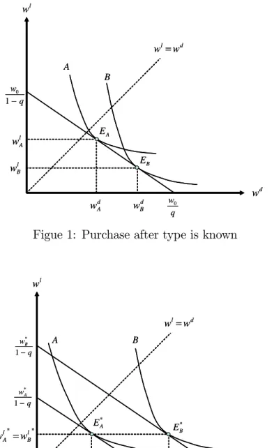
-- Fig. 1 and 2 about here
--Figures 1 and 2 provide a state-space representation of the consumer’s problem at date t = 1, when bequest type is known but one’s date of death is still uncertain. In …gure 1 preference risks are not insured. The negatively sloped straight line is the budget constraint arising from the insurer’s zero pro…t condition, i.e.,
(1 q)wli+ qwid= w0:
Indi¤erence curves (iso-expected-utility) for both bequest types are shown. For bequest type i, the marginal rate of substitution between wealth in the surviving state and wealth in the death state is
dwl i dwd i = qv 0 i(wd) (1 q)u0(wl):
For each type, the equilibrium occurs at the tangency point with the budget
wd
B > wAd and wBl < wlA, leading to equilibria such as the contingent claims
EA and EB in …gure 1.4
Figure 2 illustrates the case where preference risks can be insured. The date 1 budget constraint is then
(1 q)wil+ qwid= wi; i = A; B:
The equilibrium contingent claims in this case are EA and EB characterized
by the condition wl
B = wAl . Moreover, wdA is smaller and wBd larger than the
corresponding amounts in the uninsured case.
Of course, direct insurance against bequest type is not feasible if one’s bequest type is unveri…able. An individual purchasing such a policy would always want to claim that he is the high bequest type in order to receive the
indemnity Q . This is obvious from …gure 2. Rather than staying at EA,
a type-A individual is better o¤ claiming he is B and moving to the higher budget line.
4
Bequest type is unveri…able
We now turn our attention to the case where bequest type is private infor-mation and show how we can improve upon the naïve strategy of waiting until date t = 1 to purchase insurance. Note that it does not matter whether or not type is veri…able by the insurer to implement the naïve strategy.
Long-term life insurance contracts are purchased at date t = 0, before individuals know their bequest preferences. Many extant life insurance con-tracts often include provisions that allow for changes to the contract at some future date, at the option of the insured. One such type of provision is an opting out opportunity: the insured can trade-in his policy at a later date
4See Karni (1985) for a general treatment of models using such state-dependent
at some pre-speci…ed buy-back price. Alternatively, the contract can include an option for the purchase of additional coverage at some pre-speci…ed rate. We show that such long-term insurance contracts can improve the individ-ual’s welfare even though bequest types are non-veri…able. In particular, a well designed policy allows wealth to e¤ectively be transferred from type-A individuals to type-B individuals.
Opting out contracts
We consider a contract with a sell back option. We de…ne the contract by the triplet (P; L; K), where P denotes the premium paid at t = 0, L denotes the death bene…t and K is the price at which the policy can be traded in (i.e. sold back to the insurer) at date t = 1. With insurers earning zero pro…t, if only type-A individuals sell back their policies, such a contract will
e¤ectively transfer the amount qL K from type-A individuals to type-B
individuals at date t = 1. In essence, the insurer sells the original coverage
Lat a subsidized price. The insurer …nances this subsidy by buying back the
policy at an unfair price from the low-bequest types, who then subsequently purchase a lower level of coverage.
Such an arrangement works if the following three incentive-compatibility conditions are satis…ed:
(a) type-A individuals choose to sell back their policy at t = 1 and buy a
new short-term policy on the “spot” market at actuarially fair prices5:
VA(w0 P + K) qvA(w0 P + L) + (1 q)u(w0 P ): (7)
5We make the usual assumption that an individual chooses the action designed for him
(b) type-B individuals prefer keeping their policy at t = 1:
qvB(w0 P + L) + (1 q)u(w0 P ) VB(w0 P + K): (8)
(c) From the perspective of date t = 0, the arrangement dominates the
strategy of waiting until t = 1 to buy insurance:
U (1 )VA(w0) + VB(w0); (9)
where U denotes the expected utility provided by the long-term contract
U (1 )VA(w0 P +K)+ [qvB(w0 P + L) + (1 q)u(w0 P )] : (10)
In addition, the contract must yield a non-negative pro…t:
P qL + (1 )K: (11)
It is easily seen that the set of contracts that satisfy the above constraints
is not empty. In particular, consider the contract de…ned by L = LB(w0)and
P = K = qLB(w0), where LB(w0) is the optimal death bene…t for type B
under the naïve strategy. The non-negative pro…t condition and (8) are then satis…ed as equalities, and (7) is satis…ed as a strict inequality. Clearly, this arrangement yields the same outcome as the naïve strategy described in …gure 1, implying that (9) is then satis…ed as an equality.
In a competitive market, insurers are led to o¤er the best contract subject to pro…ts being non negative. The equilibrium contract is therefore the one that maximizes U de…ned as in (10) subject to the non-negative pro…t condi-tion and the incentive compatibility condicondi-tions. Since it is a maximum, the optimal contract is at least as good as the naïve strategy, i.e., the constraint
(9) is trivially satis…ed. Also, given K P, it is easily checked that (9)
implies (8). Thus, the only relevant constraints are (7), which is the opting out condition for type A, and the non-negative pro…t condition (11).
Second-best arrangement
Under the above arrangement, type A’s wealth at date t = 1, after exercising
his option to sell back his policy, is wA = w0 P + K. This type then
purchases the optimal death bene…t LA(wA) in the date 1 market. This
yields the …nal contingent wealth levels wl
A = wA qLA(wA) and wdA =
wA qLA(wA) + LA(wA). Type B does not opt out and thus the …nal
contingent wealth allocation follows directly from the long-term insurance
contract, i.e., wlB = w0 P and wdB = w0 P + L. The date 1 value of this
allocation is
wB = qwBd + (1 q)w
l
B = w0 P + qL:
The implied wealth transfer from type-A to type-B individuals is therefore
wB wA= qL K.
Written in terms of wA, wBl and wdB, the second-best arrangement solves
the following program: max wA;wlBwdB U = (1 )VA(wA) + qvB(wdB) + (1 q)u(w l B) subject to VA(wA) qvA(wdB) + (1 q)u(wBl ) (12) and (1 )wA+ qwBd + (1 q)wlB w0: (13)
The …rst inequality is type A’s incentive compatibility constraint; the second follows from the insurer’s non-negative pro…t condition.
It is straightforward to characterize the main features of the solution to the above problem. The resource constraint (13) is obviously binding. We show …rst that the self-selection condition (12) must be binding as well. Suppose, to the contrary, that the optimal solution maximizes U subject to (13) only. This is readily seen to yield a solution
Substituting from (1) and (2), we then have
u0(wlA) = v0A(wAd) = v0B(wdB) = u0(wlB);
which corresponds to the …rst-best allocation represented in …gure 2.
How-ever, as is clear from the …gure, type A strictly prefers EB to EA, implying
that type A would not opt out, i.e., (12) is not satis…ed.
Secondly, the naïve strategy is not a solution. As discussed above, (12) holds as a strict inequality under the naïve strategy. Since this condition must bind, the naïve strategy does not solve the problem. However, since it nevertheless satis…es the constraints, it must be the case be that the in-dividual is strictly better o¤ under the long-term contract. The following proposition summarizes these results.
Proposition 1 Long-term opting-out contracts make individuals strictly
bet-ter o¤ than the naïve strategy, but they remain second-best compared to the (complete-information) case where bequest needs are directly insurable.
Levels of coverage
We next examine how the levels of coverage di¤er under the various insurance arrangements. The Lagrangian of the second-best program is
L = (1 )VA(wA) + qvB(wBd) + (1 q)u(w l B) + VA(wA) qvA(wBd) (1 q)u(wBl ) + w0 (1 )wA qwdB+ (1 q)w l B ;
with positive multipliers and . Together with (12) and (13) holding as
equalities, the solution satis…es the …rst-order conditions
@L
@wA
@L @wd B = q vB0 (wBd) vA0 (wdB) = 0; (15) @L @wl B = (1 q) ( ) u0(wlB) = 0: (16)
Denote the solution by (wbA;wbBd;wbBl ). The date-1 value of type B’s
allo-cation iswbB qwbBd+ (1 q)wblB. Type A’s allocation iswbAd andwbAl satisfying
v0A(wbAd) = u0(wblA) = VA0(wbA): (17)
An illustration is given in …gure 3. We derive two results. First, the wealth transfer from type-A to type-B individuals in the long-term arrangement is smaller than in the …rst-best contract. Secondly, the second-best contract provides a greater death bene…t than type B would wish if he could purchase freely on the basis of his contractually de…ned date 1 wealth.
-- Fig. 3 about here
--Wealth transfer. We show that the subsidy from type-A to type-B
individuals is lower in the second-best solution vis-à-vis the …rst-best one: b
wB wbA< wB wA. Suppose, to the contrary, that
b
wB wbA wB wA: (18)
From the zero-pro…t condition, the state wealth levels satisfy
(1 )wbA+ wbB = (1 )wA+ wB = w0:
Hence, (18) implies wbA wA and wbB wB. A’s date-1 budget line in the
second-best arrangement is then below the …rst-best one represented in …gure 2, while B’s budget line would be above the one in …gure 2.
A’s allocation satis…es (17). Since bequest and survival wealth are normal
allocation. This is given by the intersection of A’s indi¤erence curve through (wbd
A;wbAl ) and B’s budget line. Obviously, the foregoing implies wbBd > wBd .
Combining both these results yields
vA0 (wbdA) vA0 (wdA) = v0B(wdB) > vB0 (wbBd), (19) where the equality follows from the optimality conditions for a …rst best.
We now turn to the restrictions imposed by the …rst-order conditions. From (14) and (15) it follows that
vB0 (wbBd) = 1 + 1 V 0 A(wbA) + v0A(wbBd): (20) Substituting for V0 A(wbA) = vA0 (wbdA) from (17), (20) implies vB0 (wbdB) > vA0 (wbdA)
which contradicts (19). The wealth transfer must therefore be strictly smaller in the second-best arrangement.
Distortion. Here we show that the B-type is forced to "overinsure,"
which can be interpreted as a type of signalling cost in the second-best
set-ting. This distortion is represented by a point such as bEB in …gure 3. As
drawn, the long-term contract provides a larger bequest (and correspondingly smaller survival wealth) than type B would wish to puchase voluntarily on
the basis of the post-transfer wealth level wbB. In other words, L > LB(wbB)
or equivalently wbdB >wbB qLB(wbB) + LB(wbB). This is a necessary feature
of the second-best arrangement. The intuition is that this “distortion” fa-cilitates the transfer of wealth from state A to state B, by making it more costly for type A not to opt out of the initial contract.
To see this more formally, substituting from (15) and (16) yields vB0 (wbBd) u0(wblB) = vA0 (wbdB) u0(wblB) :
No “distortion” would require that the left-hand side is zero, which in turn
through bEB cannot be steeper than the fair-odds line. Otherwise, a pair
(wd
B; wlB) could be chosen on the same fair-odds line below A’s indi¤erence
curve through bEB that satis…es A’s incentive compatibility constraint and
is strictly preferred by B. Hence, we must have L larger than LB(wbB) as
claimed.
The next proposition summarizes our results.
Proposition 2 Under the second-best long-term contract
(i) the wealth transfer between type A and type B is smaller than the …rst-best transfer and
(ii) high-bequest types are over-insured relative to the coverage they would like to have at the contractually de…ned wealth level.
The foregoing results imply that type-A’s bequest and survival wealth are greater than in the …rst best, while type-B’s survival wealth is smaller. However, how type-B’s bequest compares with the …rst-best level is ambigu-ous. There are two opposing e¤ects so to speak. On the hand, because of the distortion, B’s equilibrium bequest is larger than he would wish at the wealth
level wbB. On the other hand, his wealth level is lower than the …rst-best wB.
When conditional wealth levels do not di¤er too much from the …rst best, it may therefore be that B leaves a larger bequest. In this case, bequest by both types are greater than in the …rst best.
It is interesting to note that at date 1, an individual who turns out to be type A will be better o¤ with the second-best contract than with the …rst-best
one. This is to be expected, since the subsidy is lower under the
second-best arrangement. In other words, at date 0 the individual would prefer
the extra protection a¤orded by a larger subsidy. However, an individual
who eventually turns out to be of a low-bequest type will be happier if the subsidy is smaller when date 1 arrives.
Opting in contracts
An alternative to the opting out arrangement is to o¤er a contract with an option to purchase additional coverage at date t = 1. Such an "opt-in" contract is de…ned by the vector (P ; L; S; k) where P is the premium paid at t = 0 for coverage L and S is the optional additional coverage that the
individual can purchase at date t = 1 for an additional premium k. If
P > qLand k < qS, then wealth will be transferred from type-A individuals
to type-B individuals, provided of course only type B exercises the option to purchase additional coverage. Here, the original coverage L is sold at an
unfair premium. The non-negative pro…t constraint under this opting-in
arrangement is
P qL + (qS k): (21)
The above contract is equivalent to selling both types an initial contract with death bene…t (L + S) for a premium of (P + k). The type-B individual "opts in" by maintaining this package at date t = 1. The type-A individual refuses to "opt in" at date t = 1 by obtaining a refund of the extra premium k, and reducing the death total bene…t by an amount S. As before, e¤ectively only the A-type’s incentive compatibility constraint matters, with the type-A individual being just indi¤erent between opting in or not opting in.
De…ning
P P + k; L L + S and K qL + k; (22)
it is easily seen that the non-negative pro…t constraint (21) is equivalent to the previous non-negative pro…t constraint (11), and it will be satis…ed once again with an equality at the optimum. We have one additional requirement here, namely that a type-A individual who would receive a refund qL+k at date t =
1would purchase an optimal level of insurance coverage LA(w0 P +qL) = L,
…rst-order condition for LA, this requires that
vA0 (w0 P + qL qLA+ LA) = u0(w0 P + qL qLA) (23)
be satis…ed when LA(w0 P + qL) = L.
It then follows in a straightforward manner that the same triple (P; L; K) is optimal, which together with (22) and (23) determine the parameters for the optimal opt-in contract: (P ; L; S; k). Thus, the opting-in and opting-out
arrangements are e¤ectively identical.6
5
Concluding Remarks
This paper has shown how a long-term insurance contract can be designed, within a competitive insurance market, to insure the uncertain future bequest needs of the individual. We derived two equivalent forms for this long-term
insurance contract:7
(i)It provides a high level of initial coverage at a subsidized (low) price,
with an option to sell back the policy at an unfair price (i.e. at a loss to the insured)
or
(ii) It provides a low level of initial coverage at an unfair (high) price,
with an option to purchase additional coverage at a subsidized (low) price.
The existence of such contracts in the market place depends crucially
on the self selection of types in exercising the various options. But some
6One can also verify this directly by writing out the incentive compatibility constraints
and then …nding the optimal (P ; L; S; k) directly, which together with (23) shows the equivalence of the two types of contract arrangements.
7These two forms will not be unique. For example, an intermediate level of insurance
could be o¤ered with both "opt in" and "opt out" opportunities to achieve the same …nal wealth levels.
relatively new innovations in the …nancial marketplace may have an
unto-ward e¤ect on the development of the long-term contracts we propose. In
particular, the market for life settlements poses such an obstacle.
A life settlement contract essentially o¤ers to "buy back" the life
insur-ance policy of an individual.8 This is e¤ected via a third party paying cash to
the insured, in exchange for being named the bene…ciary of the life insurance death bene…t. Although this seems to eliminate any bene…t to the original bene…ciary, this will not be the case. In particular, under contract (i), the low-bequest need individual will opt to sell the policy to a life settlement broker, rather than back to the insurer, and receive more money for the pol-icy. The insured can then purchase insurance at a fair price, since there is no insurability risk. Under contract (ii), both bequest types might purchase the additional extra insurance at the low price, with the low-bequest need type individual then immediately selling back the extra coverage in the life settlement market for a pro…t.
The existence of such markets provides an alternative for the insured that is bene…cial ex post (i.e., after signing the original long-term contract). Insurance companies had originally protested as these markets developed, claiming that they should have the exclusive right to buy-back (i.e. "settle")
contracts that they had written. But others disagree. For example,
Do-herty and Singer (2002) tout the bene…ts of life settlement markets to the
insurance consumer. Such analysis might be incomplete, however, in that
it excludes the fact that ex ante (i.e. prior to learning one’s bequest type) one would prefer the longer term contracts described in this paper; and the life settlement market might preclude such contracts from ever being o¤ered.
8A similar arrangement is a viatical settlement, which is exclusively for people who are
terminally ill. See Doherty and Schlesinger (2000) and Doherty and Singer (2002). Since the viatical-settlement market depends critically on a large change in the insurability risk, the life settlement market is more appropriate here.
Although the long-term contracts we describe in this paper give the insurer monopoly power ex post, a competitive market ex ante should ensure that insurers cannot earn undue monoply rents.
Obviously, we simpli…ed the setting of our analysis by assuming away
many complicating factors, such as the insurability risk. This allowed our
focus to be on the bequest needs and the (non-random) probability of death. Integrating these results into more complex settings is di¢ cult. Hopefully, our paper takes a good …rst step in this direction.
References
[1] Campbell, R. A. (1980). Demand for life insurance: An application of the economics of uncertainty. Journal of Finance 35, 1155-1172.
[2] Cochrane, J. H. (1995). Time-consistent health insurance. Journal of Political Economy 103, 447-473.
[3] Doherty, N. A. and Schlesinger, H. (2000). Viaticals: A matter of life and death, Unpublished Working Paper, University of Pennsylvania. [4] Doherty, N. A. and Singer, H. J. (2002). The bene…t of a secondary
market for life insurance policies, Wharton Financial Institutions Center Working Paper No. 02-41.
[5] Hendel, I. and Lizzeri, A. (2003). The role of commitment in dynamic contracts: Evidence from life insurance. Quarterly Journal of Economics 118, 299-327.
[6] Karni, E., (1985). Decision Making Under Uncertainty: The Case of State-Dependent Utility. Cambridge, MA: Harvard University Press.
[7] Lewis, F. D. (1989). Dependents and the demand for life insurance. American Economic Review 79, 452-467.
[8] Pauly, M. V.; Kunreuther, H.; and Hirth, R. (1995). Guaranteed re-newability in insurance. Journal of Risk and Uncertainty 10, 143-156. [9] Polborn, M. K., Hoy, M., & Sadanand, A. (2006). Advantageous e¤ects
of regulatory adverse selection in the life insurance market. Economic Journal 116, 327-354.
[10] Villeneuve, B. (2000). Life insurance, in: G. Dionne, Editor, Handbook of Insurance, Boston: Kluwer Academic Publishers.
A B l w d w l A w d A w l B w d B w q w − 1 0 q w0 d l w w = B E A E A B l w d w l A w d A w l B w d B w q w − 1 0 q w0 d l w w = B E A E
Figue 1: Purchase after type is known
A B l w d w * * l B l A w w = * d A w d* B w q wB − 1 * q wA − 1 * d l w w = * A E * B E A B l w d w * * l B l A w w = * d A w d* B w q wB − 1 * q wA − 1 * d l w w = * A E * B E
A B l w d w l B wˆ d A wˆ d B wˆ q wB − 1 ˆ q wA − 1 ˆ B A l A wˆ d l w w = A Eˆ B Eˆ A B l w d w l B wˆ d A wˆ d B wˆ q wB − 1 ˆ q wA − 1 ˆ B A l A wˆ d l w w = A Eˆ B Eˆ