Gradual Pattern Extraction from Property Graphs

(1)

HAL Id: tel-02446233

https://tel.archives-ouvertes.fr/tel-02446233

Submitted on 20 Jan 2020

HAL is a multi-disciplinary open access archive for the deposit and dissemination of sci-entific research documents, whether they are pub-lished or not. The documents may come from teaching and research institutions in France or abroad, or from public or private research centers.

L’archive ouverte pluridisciplinaire HAL, est destinée au dépôt et à la diffusion de documents scientifiques de niveau recherche, publiés ou non, émanant des établissements d’enseignement et de recherche français ou étrangers, des laboratoires publics ou privés.

To cite this version:

Faaiz Shah. Gradual Pattern Extraction from Property Graphs. Other [cs.OH]. Université Montpel-lier, 2019. English. �NNT : 2019MONTS025�. �tel-02446233�

(2)

THÈSE POUR OBTENIR LE GRADE DE DOCTEUR

DE L’UNIVERSITE DE MONTPELLIER

En Informatique

École doctorale : Information, Structures, Systèmes Unité de recherche LIRMM

Gradual Pattern Extraction from Property Graphs

Présentée par Faaiz Hussain SHAH

Le 16 juillet 2019

Sous la direction de Prof. Anne LAURENT

et Dr. Arnaud CASTELLTORT

Devant le jury composé de

Carmen Gervet, Professeur, Université de Montpellier Présidente Ricard Gavalda, Professeur, Universitat Politècnica de Catalunya Rapporteur Marie-jeanne Lesot, Maître de Conférence HDR, Sorbonne Université Rapporteur Claire Noy, Maître de Conférence, Université Paul Valéry Examinatrice Anne Laurent, Professeur, Université de Montpellier Directrice Arnaud Castelltort, Maître de Conférence, Université de Montpellier Co-directeur

(3)

(4)

(5)

(6)

Acknowledgements

The journey of PhD thesis is a life changing experience, i must say “a life transformation experience“. It requires a lot of patience, persistence and perseverance.

To reach at this stage, i really want to render my highest gratitude to Prof. Anne Laurent to give me this opportunity to work under her supervision. She is a real mentor. She was always available through emails and meetings whenever i needed guidance. I would also like to thank Dr. Arnaud Castelltort for his guidance at various phases of thesis and in particular sharing his expertise in experiments part of thesis.

I would like to thank Prof. Carmen Gervet for presiding the jury and i present my especial gratitude to Prof. Ricard Gavalda and Dr. Marie-jeanne Lesot for their valuable and explicate feedback on thesis report.

Finally, I am very much thankful for my family for their support; my mother, my father, my wife and sweet kids.

(7)

(8)

Résumé

Les bases de données orientées graphes (NoSQL par exemple) permettent de gérer des données dans lesquelles les liens sont importants et des requêtes complexes sur ces données à l’aide d’un environnement dédié offrant un stockage et des traitements spécifiquement desti-nés à la structure de graphe. Un graphe de propriété dans un environnement NoSQL est alors vu comme un graphe orienté étiqueté dans lequel les étiquettes des nœuds et les relations sont des ensembles d’attributs (propriétés) de la forme (clé:valeur). Cela facilite la représentation de données et de connaissances sous la forme de graphes. De nombreuses applications réelles de telles bases de données sont actuellement connues dans le monde des réseaux sociaux, mais aussi des systèmes de recommandation, de la détection de fraudes, du data-journalisme (pour les panama papers par exemple). De telles structures peuvent cependant être assimilées à des bases NoSQL semi-structurées dans lesquelles toutes les propriétés ne sont pas présentes par-tout, ce qui conduit à des valeurs non présentes de manière homogène, soit parce que la valeur n’est pas connue (l’âge d’une personne par exemple) ou parce qu’elle n’est pas applicable (l’an-née du service militaire d’une femme par exemple dans un pays et à une époque à laquelle les femmes ne le faisaient pas). Cela gêne alors les algorithmes d’extraction de connaissance qui ne sont pas tous robustes aux données manquantes. Des approches ont été proposées pour remplacer les données manquantes et permettre aux algorithmes d’être appliqués. Cependant, nous considérons que de telles approches ne sont pas satisfaisantes car elles introduisent un biais ou même des erreurs quand aucune valeur n’était applicable. Dans nos travaux, nous nous focalisons sur l’extraction de motifs graduels à partir de telles bases de données. Ces mo-tifs permettent d’extraire automatiquement les informations corrélées. Une première contri-bution est alors de définir quels sont les motifs pouvant être extraits à partir de telles bases de données. Nous devons, dans un deuxième temps, étendre les travaux existant dans la lit-térature pour traiter les valeurs manquantes dans les bases de données graphe, comme décrit ci-dessus. L’application de telles méthodes est alors rendue difficile car les propriétés classique-ment appliquées en fouille de données (anti-monotonie) ne sont plus valides. Nous proposons donc une nouvelle approche qui est testée sur des données réelles et synthétiques. Une pre-mière forme de motif est extrait à partir des propriétés des nœdus et est étendue pour prendre en compte les relations entre nœuds. Enfin, notre approche est étendue au cas des motifs gra-duels flous afin de mieux prendre en compte la nature imprécise des connaissances présentes et à extraire. Les expérimentations sur des bases synthétiques ont été menées grâce au déve-loppement d’un générateur de bases de données de graphes de propriétés synthétiques. Nous en montrons les résultats en termes de temps calcul et consommation mémoire ainsi qu’en nombre de motifs générés.

(9)

(10)

Abstract

Graph databases (NoSQL oriented graph databases) provide the ability to manage highly con-nected data and complex database queries along with the native graph-storage and processing. A property graph in a NoSQL graph engine is a labeled directed graph composed of nodes con-nected through relationships with a set of attributes or properties in the form of (key : value) pairs. It facilitates to represent the data and knowledge that are in form of graphs. Practical applications of graph database systems have been seen in social networks, recommendation systems, fraud detection, and data journalism, as in the case for panama papers. Often, we face the issue of missing data in such kind of systems. In particular, these semi-structured NoSQL databases lead to a situation where some attributes (properties) are filled-in while other ones are not available, either because they exist but are missing (for instance the age of a person that is unknown) or because they are not applicable for a particular case (for instance the year of military service for a girl in countries where it is mandatory only for boys). Therefore, some keys can be provided for some nodes and not for other ones. In such a scenario, when we want to extract knowledge from these new generation database systems, we face the problem of missing data that arise need for analyzing them. Some approaches have been proposed to replace missing values so as to be able to apply data mining techniques. However, we argue that it is not relevant to consider such approaches so as not to introduce biases or errors. In our work, we focus on the extraction of gradual patterns from property graphs that provide end-users with tools for mining correlations in the data when there exist missing values. Our approach requires first to define gradual patterns in the context of NoSQL property graph and then to extend existing algorithms so as to treat the missing values, because anti-monotonicity of the support can not be considered anymore in a simple manner. Thus, we introduce a novel approach for mining gradual patterns in the presence of missing values and we test it on real and synthetic data. Further to this work, we present our approach for mining such graphs in order to extract frequent gradual patterns in the form of “the more/less A1,..., the more/less

An" where Ai are information from the graph, should it be from the nodes or from the

rela-tionships. In order to retrieve more valuable patterns, we consider fuzzy gradual patterns in the form of “The more/less the A1is F1,...,the more/less the Anis Fn" where Aiare attributes

retrieved from the graph nodes or relationships and Fi are fuzzy descriptions. For this

pur-pose, we introduce the definitions of such concepts, the corresponding method for extracting the patterns, and the experiments that we have led on synthetic graphs using a graph genera-tor. We show the results in terms of time utilization, memory consumption and the number of patterns being generated.

(11)

(12)

List of Figures

1.1 AI in Practice and Current Dimensions [Log16, Reu16, Ful16] . . . 3

1.2 Data Mining Process [Kam09a] . . . 3

1.3 Data Mining Application Domains [HPK11] . . . 4

1.4 Data Mining Venn Diagram [Hal+14] . . . 4

1.5 Graph Type Morphisms [RN10] . . . 6

1.6 Graph Databases Overview [RWE15] . . . 7

1.7 Property Graph Representation . . . 8

2.1 DB-Engines Ranking of Graph DBMS -Trend Chart April 2019 . . . 13

2.2 DB-Engines Ranking of Graph DBMS -Tabular April 2019 . . . 13

2.3 Graph Native Storage and Processing . . . 14

2.4 Explicit relationships . . . 14

2.5 Property Graph with data as (key:value) pairs . . . 16

2.6 Running Example Graph Database Schema. . . 17

2.7 Running Example Property Graph Visualization . . . 18

2.8 Output Example Cypher Pattern Query . . . 19

(19)

2.10 The KDD Process [FPS96] . . . 21

2.11 p1 w.r.t all other tuples . . . 28

2.16 Final Binary Matrix of Order for Gradual Item (Age ↑) . . . 29

2.17 ( Age ↑ ) - Hasse Diagram Representation . . . 29

2.18 ( Experience ↑ ) - Hasse Diagram Representation . . . 29

2.19 ( Publications ↑ ) - Hasse Diagram Representation . . . 29

2.20 (Experience ↑) Binary Matrices for Gradual Item of Size-1 . . . 30

2.21 (Publications ↑) Binary Matrices for Gradual Item of Size-1 . . . 30

2.22 Binary AND of concordant object pairs for gradual patterns (Age↑ , Experience↑) 30 2.23 Precedence Graph ( Age ↑ , Experience ↑) - Hasse Diagram representation . . . 30

2.24 Binary matrix representing orders for the dataset shown in Table 2.3 . . . 31

2.25 Binary AND of concordant object pairs for gradual patterns (Age↓ , Publications↓) 32 2.26 Membership Functions [Str15]. . . 34

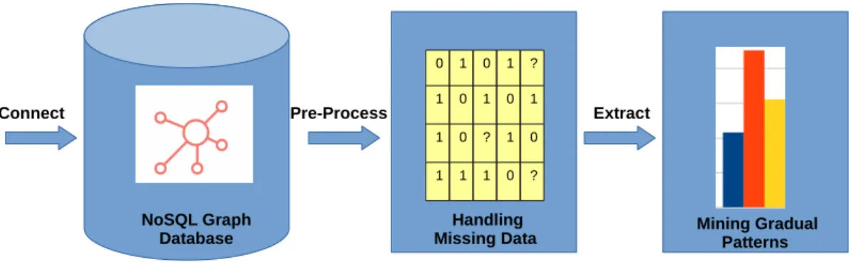
2.27 Property Graphs Missing Data Handling and Pattern Mining Process . . . 36

2.28 Handling Missing Data [Swa18] . . . 37

2.29 Datasets with and without Missing values. . . 39

3.1 Property Node . . . 45

3.2 Property Relationship between two Property Nodes . . . 45

3.3 Property Graph . . . 47

3.4 Label “Person” Nodes . . . 50

(20)

List of Figures xix

3.6 Property Graphs Gradual Pattern Mining Process . . . 53

3.7 Fuzzy Partition . . . 59

4.1 Binary matrix representing orders for Table 4.3 . . . 64

4.2 Hadamard product for binary AND operation of Age AND Expr . . . 65

4.3 Neo4j Internal Architecture . . . 70

4.4 Extension possibilities . . . 72

4.5 API Service Illustration . . . 73

4.6 Neo4j: run of Intra-Label-Node-Properties GP with on a label . . . 77

4.7 Neo4j: run of Intra-Label-Node-Properties GP with on a label and minsup . . . . 77

4.8 Neo4j: run of Intra-Label-Node-Properties GP with on a label and minsup + skipProperties . . . 78

5.1 Graph Data Generation tool . . . 81

5.2 Synthetic Graph Generator for Neo4j . . . 81

5.3 Graph Tool Parameters Descriptions . . . 83

5.4 Cypher with Random Names of Labels, Relationships and Properties . . . 85

5.5 Original Graph Generator Tool with Cypher . . . 89

5.6 Uniform Nodes and Relationships "Without" Properties in Original Graph Gen-erator . . . 90

5.7 Non-uniform Nodes and Relationships "Without" Properties in Original Graph Generator . . . 90

5.8 Explicit Label Names Nodes "With" Properties in Extended Graph Generator . . 91

5.9 Explicit Relationship Names Nodes "With" Properties in Extended Graph Gen-erator . . . 91

5.10 Random Label Names Nodes "With" Properties in Extended Graph Generator . . 92

5.11 Random Relationship Names Nodes "With" Properties in Extended Graph Gen-erator . . . 92

(21)

5.12 Russian-Twitter-Troll Sandbox Details . . . 96

5.13 Russian-Twitter-Troll-Graph Schema Visualization . . . 96

5.14 Synthetic Graph Schema visualizations . . . 99

5.15 Hetnet Graph Schema visualizations [Dan19] . . . 100

5.16 Time Utilization for Russian Troll Tweets . . . 102

5.17 Memory Consumption for Russian Troll Tweets . . . 102

5.18 Number of Patterns for Russian Troll Tweets . . . 102

5.19 Time Utilization for Hepatitis - UCI ML Repository Dataset. . . 103

5.20 Memory Consumption for Hepatitis - UCI ML Repository Dataset. . . 103

5.21 Number of Patterns for Hepatitis - UCI ML Repository Dataset . . . 103

5.22 Time Utilization for Synthetic Dataset . . . 104

5.23 Memory Consumption for Synthetic Dataset . . . 104

5.24 Number of Patterns for Synthetic Dataset . . . 104

5.25 Time Utilization for Synthetic Graph Generator Dataset . . . 105

5.26 Memory Consumption for Synthetic Graph Generator Dataset . . . 105

5.27 Number of Patterns for Synthetic Graph Generator Dataset . . . 105

5.28 Time Utilization for Hetionet(Gene) Dataset Dataset . . . 106

5.29 Memory Consumption for Hetionet(Gene) Dataset Dataset . . . 106

5.30 Number of Patterns for Hetionet(Gene) Dataset . . . 106

5.31 Time Utilization with Fuzzy Sets . . . 107

5.32 Memory Utilization with Fuzzy Sets . . . 107

5.33 No. of Patterns with Fuzzy Sets . . . 107

5.34 Time Utilization for Crisp Data . . . 107

5.35 Memory Utilization for Crisp Data . . . 107

(22)

List of Figures xxi

6.1 Cache and Filesystem . . . 113

A.1 (vdb) approach . . . 129

(23)

(24)

List of Tables

2.1 Most Used Neo4j Cypher Clauses . . . 15

2.2 Market Basket Dataset . . . 23

2.3 Person Data . . . 28

3.1 Label “Person” Tabular form . . . 50

3.2 Age Fuzzy Sets . . . 59

3.3 Data Fuzzification . . . 60

4.1 |vdb (Age)| . . . 62

4.2 |vdb (Sal)| . . . 62

4.3 Retrieved Data from Graph for Age & Expr . . . 63

4.4 |vdb (Age & Expr)| . . . 64

4.5 |vdb (Age & Sal)| . . . 64

4.6 |vdb (Age & Sal & Expr)| . . . 64

5.1 Intra-Node Gradual Pattern Mining . . . 95

5.2 Nodes with Relationships Gradual Pattern Mining . . . 96

5.3 Hetionet “Gene”Relationships Summary . . . 100

(25)

(26)

Chapter

1

Introduction

1.1 Introduction . . . . 2 1.2 Problem Statement . . . . 8 1.3 Thesis Outline . . . . 9

(27)

1.1 Introduction

With the provision of ever increasing data rates on Internet and open source technologies to the end users, it has become increasingly challenging for many enterprises to process large vol-umes of data in an efficient manner. In some cases, traditional database management systems may not be able to store, process, manage, and analyze data to get insight of data for efficient decision making.

Since the inception of artificial intelligence (AI) in 1956 at Dartmouth conference, it has be-come such an important field that its influence on our daily lives can hardly be overestimated [Lun+07]. The rapid change in AI technologies is transforming various aspects of our lives and human activities from healthcare to education, supply chain, manufacturing, entertain-ment, etc. It has evolved from simple rule-based systems to machine learning in 1980s to deep learning in recent days and it is continuously evolving into many more aspect of information technology. Thomson Reuters, a well know corporation that serves the decision makers in providing integrated and intelligent information on financial risks for businesses and profes-sionals states “experts predicts that spending on AI by companies will grow from $8 billion in 2016 to $47in 2020, up almost 600%” [Reu19]. The current AI practices and state of the art is shown in Figure1.1.

Artificial intelligence, data mining, and machine learning techniques are being actively studied for last three decades. More and more applications have been developed these days at a scale to solve the problems in diversified fields including computer science (neural nets and deep learning), medical science (biological databases), chemistry (DNA sequencing and molecules properties analysis), physics (quantum machine learning and experimental physics e.g. Large Hadron Collider experiments at CERN), space technology (data streams or sensor readings) etc. One of the main purpose of all these developments is to emulate human intelli-gence and implement or apply decision making process for computers.

At the crossroads of big data and artificial intelligence, the objective of data mining can be precisely described as “the non-trivial extraction of new, implicit, and actionable knowledge from large datasets” [WHR98]. Formally, it can be defined as “a process concerned with uncovering patterns, associations, anomalies, and statistically significant structures and events in data” [Kam09b]. The process involves collecting raw data, cleaning, pre-processing, data transformation into desired formats and then extraction of patterns to gain useful insight from data. The key steps in the process of data mining are briefly shown in Figure1.2.

As stated in [HPK11], data mining is a highly application-driven domain that has adopted many techniques from various domains such as “statistics, machine learning, pattern recognition, database and data warehouse systems, information retrieval, visualization, algorithms, high-performance computing, etc.,”. Figure 1.3depicts the relationships of data mining with different domains, where each one of them is entirely as vast field of research. Figure1.4given in article [Hal+14] shows the Venn diagram representation of AI, data mining, machine learning, and particularly

(28)

1.1. Introduction 3

Figure 1.1 –AI in Practice and Current Dimensions [Log16,Reu16,Ful16]

data science domain covering databases, statistics, and pattern recognition as well as others. This clearly shows the versatility of data mining domain as well as the complexity involved in a particular mining task. The advantage of this intersection of data mining with several fields make it a source to deal with many open research problems.

The applications of data mining are often closely related to one of four main problems i.e., pattern mining, clustering, classification and outlier analysis [Agg15b]. The data mining pro-cess may vary depending on the type of data and the level of complexity for data analysis. It involves to find the relationships between attributes/columns and relationships between ob-jects/rows. Pattern mining (aka association pattern mining) and classification are generally

(29)

Figure 1.3 –Data Mining Application Domains [HPK11]

Figure 1.4 –Data Mining Venn Diagram [Hal+14]

used to find relationships between attributes, whereas clustering and outlier analysis find rela-tionships between objects [Agg15b]. In data mining, the overall goal is to transform raw data into understandable structures that are presentable in such a way that they may be used for predictive analysis and strategic or capacity planning.

Pattern recognition is one the key step of data mining as shown in Figure1.2. It involves considering various algorithms for an application to implement it in such a way to make the application more effective and computationally efficient [Kam09a]. A pattern is defined as “an arrangement or an ordering in which some organization of underlying structure can be said to exist. Patterns in data are identified using measurable features or attributes that have been extracted from the data.” [Kam09a]

(30)

1.1. Introduction 5

Pattern mining is generally referred as frequent itemsets (pattern) mining or frequent sub-sequence (sequential patterns) mining. It is used to find the items that appear often together and in some sequence in transactional dataset [HPK11]. The data classification mining de-termines the relationships of a special column with other columns of dataset and hence the process is referred to as supervised. In clustering the main objective is to determine how the values of a subset of rows are related to the values in corresponding columns. The outlier anal-ysis refers to “identify entries in the rows are different from the corresponding entries in other row”, and it becomes interesting data or unusual data point [Agg15b].

Frequent pattern mining i.e., mining the data patterns having more occurrences than a pre-defined threshold is a major domain in data mining. Frequent pattern mining has rapidly extended from transactional databases analysis to the analysis of complex structures having numerical attributes such as sequences, trees or graphs. Therefore, frequent gradual pattern mining poses a new challenge to design efficient algorithms capable of scaling up on huge and complex databases [DLT09].

Gradual pattern extraction is the process of discovering knowledge from databases as com-parable attributes of co-variations. These can be increasing variations or decreasing variations. In linguistic expression, it may be represented as, “the more/less the value of Xi,. . . , the

more/-less the value of Xn”, where i = 1, 2, 3...n, and X1,X2,X3, . . . to Xn are numerical ordinal

at-tributes [DLT09]. For instance, a gradual pattern is considered interesting if it occurs frequently i.e., the support of that pattern is greater than the given threshold (minimum support).

Efficient mining of gradual patterns from large numerical databases is a non-trivial task, in particular when considering the scalability issues due to ever increasing volume of data in enterprises. The application of gradual patterns mining can be found in various fields rang-ing from applications for analyzrang-ing client databases for marketrang-ing purposes, analyzrang-ing pa-tient databases in medical studies, analysis of climate and environment change. The existing gradual pattern mining techniques presented in [DLT09,LLR09,Do+15] are mainly for tabular databases while some other types are emerging, as for instance property graphs.

The concept of graph is studied since late 19thcentury, however, in last few decades in the field of computer science, the research in applied graph has grown due to prevalence of social networks and networked-based data [RN12]. “A graph G = (V,E) is a data structure composed of a set of vertices (V) and edges (E)” or more commonly called as a set of nodes and the relationships that connect them [RN10]. The authors in [RN12,Rod16] present various types of graphs by describing their relevant definition as shown in Figure1.5.

Graphs provide us better understanding of diversified datasets in the fields such as science, government, and business [FG17, Muñ+17]. As stated in [RWE15], “The expressive nature of graph structures allows us to model almost all kind of scenarios for computing like construction of a space rocket, system of roads, supply chain, medical history for populations, etc”. This expressive nature of graph structures helps to model a vast number of real scenarios of governments and business applications [Neo19e,Neo19c].

(31)

Figure 1.5 –Graph Type Morphisms [RN10]

Graphs have been studied from many years [Tru94] but they have only been integrated in database engines in recent years with the so called name as “graph databases”. In contrast with relational database, there is no concept of “joins” in a graph database and relationships are treated as first class citizens [RWE15]. When considering the graph database technologies there are two main properties of a graph database are (i) underlying storage i.e., the way in which graphs are stored and manged and (ii) graph processing engine i.e, the way in which graph queries are processed, typically as an index-free node traversal [RN12,RWE15]. The Figure1.6

shows an overview of graph database present with respect to these two properties.

Graph modeling helps to identify people’s interactions, influences, and exchange of ideas on these social networks has helped to better understand global demographics, political move-ments and products commercialization [Van14]. Graph modeling is generally an iterative pro-cess. A property graph data model enables to represent the data in a natural way with the flex-ibility to incorporate schema changes as and when required. It does not require a fixed schema prior to the database creation. Hence, it is also referred as semi-structured data. In graph the-ory, these types of graphs are called “dynamic” or “time-evolving” graphs, where changes occur in vertices and edges over the time [KBB17,Dem+10,Liu+18]. For building a property graph model, first we identify requirements for the node labels and relevant properties that are to be assigned to nodes. Then we identify and assign the relationships between these nodes and their properties. This process becomes and evolutionary process and nodes and relationships keeps on adding as and when required.

(32)

1.1. Introduction 7

Figure 1.6 – Graph Databases Overview [RWE15]

Graph data can be embeded within NoSQL graph oriented databases. The other categories of NoSQL databases include Key-Value store, Column-Family stores, and Document stores re-spectively. Many companies have developed their in house implementations of graph database systems such as, Facebook’s Open Graph, Google’s Knowledge Graph, FlockDB by Twitter, and many more [Mil13]. The other open source graph database solutions are Dex, InfiniteGraph, and OrientDB having different levels of maturity. NoSQL graph engines are purpose built sys-tems to store nodes and relationships natively. Nodes or vertices (data entities) are created and linked through relationships (edges), that results in much faster query response for this linked data. The increasing need for such systems has been observed in use cases including “social networks, recommendation engines, knowledge graphs, fraud detection, network and IT operations, and life sciences”[Beb+18].

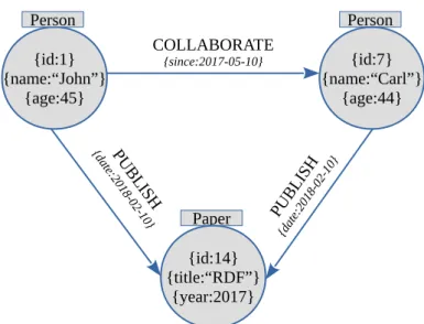
A property graph is a way to represent data as graphs. “In the parlance of graphs, a prop-erty graph is a directed, edge-labeled, attributed multi-graph”[RN12]. A property graph is typically defined as a data model in a graph structure containing nodes and relationships with proper-ties/attributes in form of (key:value) pairs. Nodes are represented as entities and relationships are the edges that connect these entities. A node can have one or more Labels that define the role of a node. Relationships between two nodes have one Type; they are directional and may contain (key:value) properties as nodes as shown in Figure 1.7. Several relationships can be defined between two nodes, which is different from regular graphs.

(33)

Collaborates {key:value} Paper

key:value

Person : Student Person : Professor P ub lis_h {key :val ue} {k_ey :va_lu e} key:value key:value Publ ish

Figure 1.7 – Property Graph Representation

1.2 Problem Statement

In recent years, graph data management and mining is gaining a lot of interest in database research community due to its pervasiveness in the fields such as, social networks, knowledge graphs, genome and scientific databases, medical and government record [KBB17]. Also, the research is being actively pursed for last one decade in gradual pattern mining from large nu-merical tabular datasets along with addressing the scalability issues [DLT09,LLR09,Ayo+10,

QLP11, Do+15, AY14, Lau+12, Ngo+18]. This dissertation argues that in case of property graphs, it is not possible to apply directly existing methods for gradual patterns extraction. There are two main reasons:

1. Graphs are not same as tabular data in their meaning and application;

2. Graphs are semi-structure nature of data.

The existing techniques were primarily for small or large single dataset of tabular data without involving relationships. Also, the existing techniques did not address the issue of missing values in datasets, if they appear in attributes. In property graphs, we have nodes with label(s), that have properties/attributes (missing and non-missing) and directed relation-ships. This arises many questions like how to manage different labeled nodes data for gradual pattern mining, what to do when nodes involve relationships between them and how to do transformation into tabular data, as well as treatment of missing data, if there exist any. To the best of our knowledge, the extraction of gradual patterns from property graphs is a novel idea and has not been studied as yet. The objective of this research work is to address following two main aspects:

1. Defining gradual patterns in the context of property graphs;

(34)

1.3. Thesis Outline 9

In order to achieve these objectives, we address the issue of missing data that arises as a conse-quence when we are mining graph data. Furthermore, we also define and describe our method for mining fuzzy gradual patterns from property graphs.

We will investigate in detail each of the above mentioned aspect in the coming chapters including extending existing gradual pattern mining algorithms, their implementation results on real and synthetic graph data and discussions to highlight use and application of property graphs.

1.3 Thesis Outline

The rest of the thesis document is organized as follows.

Chapter2describes the preliminary concepts and definitions about property graphs, grad-ual patterns, mining fuzzy gradgrad-ual patterns, and various types of missing data types and the techniques for handling missing data. All these concepts are discussed as a basis to for our proposed approach presented in chapter3.

In chapter3, we describe an overall mining process for gradual patterns in the context of property graphs. A property graph is a data structure containing nodes and relationships with properties in (key:value) format. One of our contributions is to propose a formal definition of property graphs as the literature often proposes definitions that do not embed all particular-ities that we would like to include. We then introduce different forms of gradual patterns in the particular context of such property graphs. Five types are proposed that can be seen as protoforms in the sense of fuzzy summaries. Finally, we propose an extension to fuzzy gradual patterns in order to be able to extract more understandable knowledge. Such patterns can be like the more the age is “almost 40”, the more the experience is “almost high”.

In chapter4, we investigate in detail the mining of gradual patterns. Such a process implies to deal with the presence of missing values as it is in the context of property graphs. We discuss the support computation process and the algorithms with related explanations. This chapter is concluded by a section discussing how our work can be integrated in a graph database engine with by a proof-of-concept example.

In chapter 5, we show the experiments and results for our proposed approach. It starts with describing synthetic graph generator tool in detail including its implementation and how it can be used to generate property graphs in NoSQL engine like Neo4j. This GUI-based tool facilitates to generate property graphs for our experiment. Then we describe the setup environ-ment and program execution protocol. We show the details for 8 different datasets on which the experiments are led along with briefly describing them. For all these datasets the results are provided in terms of time utilization, memory consumption and the number of generated patters in the process of mining gradual pattern. The chapter ends with a discussion on the

(35)

results.

In chapter6, we present the conclusion of the entire work covering of all the chapters. In perspectives, we discuss the possible dimensions of the current work by briefly describing the conceptual visualization that could possibly lead to complete research projects.

(36)

Chapter

2

Related Work

2.1 Introduction . . . 12 2.2 Graph Databases . . . 12

2.2.1 Neo4j Graph Database . . . 12

2.2.2 Cypher Query Language . . . 15

2.3 Property Graphs . . . 15

2.3.1 Schema-less Nature of Property Graphs . . . 16

2.3.2 Graph Pattern Matching . . . 19

2.4 Gradual Pattern Mining . . . 20

2.4.1 Frequent Pattern Mining. . . 22

2.4.2 Anti-monotonicity Property. . . 24

2.4.3 Association Rules and Gradual Dependencies . . . 24

2.4.4 Formal Definition of Gradual Pattern (Itemset) . . . 25

2.4.5 Support Measure for Gradual Pattern . . . 26

2.4.6 GRITE Algorithm. . . 27

2.4.7 GRAANK Algorithm. . . 31

2.5 Fuzzy Gradual Patterns . . . 32

2.5.1 Fuzzy Logic and Fuzzy Sets . . . 33

2.5.2 Defining Fuzzy Gradual Patterns. . . 34

2.6 Handling Missing Values . . . 36

2.6.1 Handling Missing Data Techniques . . . 37

2.6.2 Handling Missing Data With Replacement . . . 38

2.6.3 Handling Missing Data Without Replacement . . . 38

(37)

2.1 Introduction

This work deals with property graphs, gradual patterns, extending fuzzy gradual patterns and missing data management. In this chapter, we will first review existing works related to these topics. In section 1.1, we briefly described about the graphs, graph database, prop-erty graphs in Neo4j graph database and the purpose to choose it to perform gradual pattern mining. Furthermore, we describe and define property graphs, state of the art about gradual pattern extraction algorithms and gradual pattern mining from property graphs. We also de-scribe mining fuzzy gradual patterns from property graphs and treatment of missing data in property graphs so as to mine gradual patterns.

2.2 Graph Databases

Graph databases have given a new way of modeling and traversing interconnected data and have applications in social graphs, recommendation systems, and bioinformatics [Mil13]. A comparison between the relational databases and graph databases focusing on the aspects of data structures, data models, query facilities and limitations of is presented in [Mil13]. The decision to choose between the relational database and graph database is primarily based on the requirements of systems that may be utilizing these database.

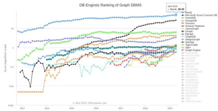
A NoSQL database engine is a system specifically designed to store, manage, and pro-cess such kind of graph-like data. Such kind of systems are gaining attention as mentioned in [SA11] "increasing usage of graph data structure for representing data in different domains such as: chemical compounds, multimedia databases, social networks, protein networks and semantic web." To-day, the well known NoSQL database systems are: Amazon’s Neptune [Ama19], Microsoft’s Cosmos [Mic19], Titan [Aur19], and Neo4j [Neo19a]. DB engine ranking [DBE19] provides the current ranking of graph database engines in the market according to the popularity and is updated monthly. The chart and list depiction of April 2019 are shown in Figures 2.1and 2.2

respectively. This clearly shows that Neo4j is a leader in Graph databases for quite some time. Therefore, based on research survey, popularity and more importantly of being open source, we choose Neo4j as graph database engine to create property graphs and apply gradual pattern mining algorithms to analyze the patterns and evaluate the results.

2.2.1 Neo4j Graph Database

Neo4j is an open source NoSQL graph database implementation that is highly scalable and leverages data as well as relationships. Neo4j stores data as connected data that provides the flexibility of adding a new node or a new relationship without compromising or migration of existing data. Relationships are considered as much important as the nodes. Relationships are used to perform the node traversing thereby eliminating the need of complex join operations.

(38)

2.2. Graph Databases 13

Figure 2.1 – DB-Engines Ranking of Graph DBMS -Trend Chart April 2019

(39)

Native Graph Processing

Native Graph Storage

Figure 2.3 –Graph Native Storage and Processing

Neo4j’s native graph storage as shown in Figure2.3is used to store the data as graphs and optimized for managing graphs. “The graph processing engine is used to provide basic graph opera-tions and algorithms to deliver constant, real-time performance, helping enterprises to build intelligent applications to meet today’s evolving data challenge” [RWE15]. Another main performance char-acteristic of a graph database is the graph traversal or pattern matching query independent of the data set size. This is achieved primarily due to native storage of data as graphs.

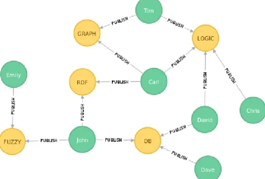
Graph traversal across the nodes using relationships is one of the key features of graph databases. Neo4j does not require a join operation because every node in graph has an explicit relationship joined between two nodes and it only requires traversal across the graph to match the required pattern. This feature results in efficient query performance and better response time. In the case of relational database systems, we need to create a separate link table in which we store foreign keys of two tables to link them together. Another advantage of property graph model as compared to relational model is that it does not require creating a schema prior the creation of database. It allows more flexibility to incorporate schema changes as and when required. J ohn Carl Dave Chris T im COLAB

Figure 2.4 –Explicit relationships

Neo4j helps to model dynamic complex relationships in a maneuverable form of connected data that can be easily understandable like white board model. Neo4j is gaining more interest in the field of data science, specifically for defining complex join-intensive and path traversal queries over the graph [RWE15].

(40)

2.3. Property Graphs 15

2.2.2 Cypher Query Language

Neo4j is a NoSQL graph database that uses “Cypher’’, a declarative query language that uses ASCII-art syntax. The queries written in declarative query language allow to declare a required pattern to retrieve data from the database as opposed to imperative query language such as SQL where we have to specifically tell the database what to do in order to retrieve the required data. Cypher query language is composed of specific clauses to perform queries from graph database.

Table2.1shows the different clauses used to query the graph data in Noe4j. Cypher uses these clauses to change or update the graph data by adding or removing the nodes, relation-ships and properties of a graph. Cypher also provides several aggregate functions to calculate aggregate data analogous to ’GROUP BY’ in SQL. These include but are not limited to COUNT, COLLECT, AVG, MAX, MIN, SUM, etc.

Clause Purpose

MATCH To match the required pattern for result RETURN To return the matched data

WHERE Provides criteria for filtering pattern matching results CREATE Create nodes and relationships

DELETE Removes nodes, relationships, and properties

SET Sets property values

UNION Merges results from two or more queries REMOVE Remove a label or property from node CALL Standalone call to built-in procedures

LOAD To import external files in graph database and create nodes ORDER BY To the result of return result in ascending or descending order

Table 2.1 – Most Used Neo4j Cypher Clauses

In the following section we describe property graphs using Neo4j graph database engine to explain the relavent concepts including the running example created in Neo4j.

2.3 Property Graphs

A Property Graph (PG) refers to a data model in which data has (key:value) pairs. A property graph data model enables us to represent the data in natural way in form of graph structure of vertices (nodes) and edges (relationships), as shown in Figure2.5. We use property graphs to represent data. Entities are represented as nodes or objects having one or more labels that describe the type or class of nodes and a node can have one or more (key:value) properties, hence the graph is called as a labeled property graph model. Each node can have one or more relationships that connect the nodes. Relationships have a single type and they can also store (key:value) properties. Relationships have a direction.

(41)

{id:1} {name:“John”} {age:45} Person Person Paper {id:7} {name:“Carl”} {age:44} {id:14} {title:“RDF”} {year:2017} COLLABORATE {since:2017-05-10} PU BL IS_H {d ate :20 18 -02 -10_} PUBL ISH {dat e:20 18-0 2-10 }

Figure 2.5 – Property Graph with data as (key:value) pairs

Property graph modeling is generally an iterative process that provides a flexibility to change the graph schema without altering the existing graph structure. This feature is very use-ful particularly for agile application development. For building a property graph data model it is important to identify the nodes and what properties are relevant to the nodes that are to be assigned. This is generally termed as user requirement gathering for developing the initial graph structure. We identify the uniquely identifiable able attributes to define the indexes and constraints accordingly. Then we identify the relationships between these nodes and possible properties these relationships can have between each node. This process is repeated whenever needed.

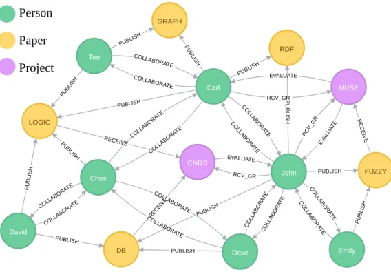
To present the definitions, we create a running example property graph in Neo4j. The graph schema of the property graphs is shown in Figure2.6showing three labeled nodes with rela-tionship types. The overall property graph visualization for this graph schema with nodes and relationships is shown in Figure2.7. The property graph shows 14 nodes with 3 labels namely person, paper and projects. There are 30 relationships with 3 relationship types namely collab-orate, publish and receive_grant.

2.3.1 Schema-less Nature of Property Graphs

The interesting thing is the property graph is that there is no fixed schema and any node(s) or relationship(s) can be removed without affecting the entire graph. Only the links between associated nodes will diminish and rest of the structure will be intact. Similarly, the addition of nodes and relationships can be done on the fly whenever required. For example, in case of Person label, assume that you have a table named “Person” in a relational database and you need to add an attribute, say “Phone_Number”. To do so, you need to define the attribute first

(42)

2.3. Property Graphs 17 Person Paper Project COLLAB. PUBLISH RCV_GRANT

Figure 2.6 –Running Example Graph Database Schema

by using ALTER table and then you can add the value for the respective record. In case of property graph, there is no need to define something before for adding an attribute/property for a node (record). You just add the property right away independent of any structure as well as without affecting relationships. That is why property graphs are often referred as schema less graphs and semi-structured data graphs.

We use Neo4j cypher-shell utility to query the list of nodes for each label. The Cypher query along with the output result for label “Person” is shown in Listing 2.1. In the query we write the names of each property to make the output more presentable. Similarly, the query and output for label “Paper” is shown in Listing 2.2and for label “Project” it is shown in Listing

2.3respectively.

1 neo4j > MATCH ( n:Person )

2 RETURN ID ( n ) AS ID , n . name AS NAME, n . age AS AGE,

3 n . d e s i g AS DESIGNATION, n . expr AS EXPERIENCE,

4 n . s a l AS SALARY ;

5 +−−−−−−−−−−−−−−−−−−−−−−−−−−−−−−−−−−−−−−−−−−−−−−−−−−−−−−−−−+ 6 | ID | NAME | AGE | DESIGNATION | EXPERIENCE | SALARY | 7 +−−−−−−−−−−−−−−−−−−−−−−−−−−−−−−−−−−−−−−−−−−−−−−−−−−−−−−−−−+ 8 | 1 | " John " | 4 5 | "PR" | 1 3 | 3 5 0 0 | 9 | 2 | " Dave " | NULL | "MCF" | 7 | 2 5 0 0 | 10 | 3 | " Emily " | 3 0 | "ETU" | 5 | NULL | 11 | 6 | " Tim " | NULL | "MCF" | 1 0 | 2 8 0 0 | 12 | 7 | " C a r l " | 4 4 | "PR" | 1 4 | 3 8 0 0 | 13 | 9 | " C h ri s " | 3 8 | "MCF" | 9 | 2 6 0 0 | 14 | 1 0 | " David " | 3 2 | "ETU" | 5 | 1 4 0 0 | 15 +−−−−−−−−−−−−−−−−−−−−−−−−−−−−−−−−−−−−−−−−−−−−−−−−−−−−−−−−−+ 16 7 rows a v a i l a b l e a f t e r 1 0 ms, consumed a f t e r another 1 ms

(43)

Person

Paper

Project

RCV_GR RCV_ GR PUBLI SH P U B LIS H PUBLISH CO LLA BO RAT E C_O LL_AB O_R AT_E CO LL AB_O RA_TE PUBLISH COL_LAB ORA_TE CO LLA BO RAT E PU BLI SH C_O LL_AB O_R AT_E PUBL ISH PUBLI SH COLLABO_RATE RCV_GR PU BL_IS H PUBLISH PUBLI SH COLLABO_RATE COLL ABOR ATE CO LL AB_O RA_TE PU BL ISH COLL ABOR ATE COL_LAB ORA_TE COLL ABOR ATE PU BLI SH PUBLISH COLL ABOR ATE RECEIVE R_E C E IV_E RECE IVE EVAL UAT E EVALUATE EVALUATE John Dave Emily Tim Carl Chris David GRAPH LOGIC FUZZY RDF DB MUSE CNRS

Figure 2.7 – Running Example Property Graph Visualization

1 neo4j > MATCH ( n:Paper )

2 RETURN ID ( n ) AS ID , n . p r _ t i t l e AS TITLE,

3 n . type AS TYPE, n . year AS YEAR, n . C i t a t i o n s AS CITATIONS,

4 n . I m p a c t _ F a c t o r AS IMPACT_FACTOR ;

5 +−−−−−−−−−−−−−−−−−−−−−−−−−−−−−−−−−−−−−−−−−−−−−−−−−−−−−−−−−−−−−−−−−−+ 6 | ID | TITLE | TYPE | YEAR | CITATIONS | IMPACT_FACTOR | 7 +−−−−−−−−−−−−−−−−−−−−−−−−−−−−−−−−−−−−−−−−−−−−−−−−−−−−−−−−−−−−−−−−−−+ 8 | 1 1 | "GRAPH" | " c o n f e r e n c e " | "2 0 1 5" | 1 0 | NULL | 9 | 1 2 | "LOGIC" | " j o u r n a l " | "2 0 1 6" | 3 0 | 4.5 | 10 | 1 3 | "FUZZY" | " c o n f e r e n c e " | "2 0 1 5" | 5 | NULL | 11 | 1 4 | "RDF" | " c o n f e r e n c e " | "2 0 1 7" | NULL | NULL | 12 | 1 5 | "DB" | " j o u r n a l " | "2 0 1 6" | 5 0 | 2 | 13 +−−−−−−−−−−−−−−−−−−−−−−−−−−−−−−−−−−−−−−−−−−−−−−−−−−−−−−−−−−−−−−−−−−+ 14 5 rows a v a i l a b l e a f t e r 1 ms, consumed a f t e r another 1 ms

Listing 2.2 –Paper Node Details

1 neo4j > MATCH ( n:P r o j e c t )

2 RETURN ID ( n ) AS ID , n . p r g _ t i t l e AS PROJECT_TITLE,

3 n . amount AS AMOUNT, n . year AS YEAR ; 4 +−−−−−−−−−−−−−−−−−−−−−−−−−−−−−−−−−−−−−−+

(44)

2.3. Property Graphs 19

5 | ID | PROJECT_TITLE | AMOUNT | YEAR | 6 +−−−−−−−−−−−−−−−−−−−−−−−−−−−−−−−−−−−−−−+ 7 | 1 6 | "MUSE" | 3 0 0 0 0 | "2 0 1 7" | 8 | 1 7 | "CNRS" | 5 0 0 0 0 | "2 0 1 6" | 9 +−−−−−−−−−−−−−−−−−−−−−−−−−−−−−−−−−−−−−−+

10 2 rows a v a i l a b l e a f t e r 1 1 ms, consumed a f t e r another 1 ms

Listing 2.3 –Project Node Details

2.3.2 Graph Pattern Matching

Pattern matching e.g., "()-[]->()" is also one of the main feature of cypher to match the de-sired graph structures and to retrieve the dede-sired information pertaining to nodes and rela-tionships in a graph. An example cypher query to find a node labeled Person, whose name property value is ‘John’ and he publishes a journal paper can be written as shown in List-ing2.4. The output of this query from Neo4j console is shown in Figure2.8.

1 MATCH ( p:Person ) − [v:PUBLISH] -> ( q:Paper ) 2 WHERE p . name =" John " AND q . type =" j o u r n a l " 3 RETURN p AS PersonName, q AS Paper

Listing 2.4 –Example Cypher Pattern Query

Figure 2.8 – Output Example Cypher Pattern Query

Similarly, if we want to see all the persons who have published in a journal, the Cypher query can be written as shown in Listing2.5. The output of the query is shown in Figure2.9.

(45)

1 MATCH ( p:Person ) − [r:PUBLISH] -> ( q:Paper ) 2 WHERE q . type =" j o u r n a l "

3 RETURN p AS PersonName, q AS Paper

Listing 2.5 –All Persons who Published in Journal

Figure 2.9 – Cypher - All Persons who Publish Paper

In the whole property graph, if we like to see who is connected with whom and in what frequency of relationships, then we can use the query shown in Listing2.6. It can also be said as topology extraction in tabular form.

After discussing briefly about the property and pattern matching in property graphs, we proceed in the next section to describe the main concepts of gradual pattern mining, definitions and algorithms presented in the literature on the topic.

2.4 Gradual Pattern Mining

The knowledge discovery process was first presented in [FPS96] as shown in Figure2.10. In the process of knowledge discovery from databases, data mining is one of the key steps that involves applying algorithms in order to extract patterns. Data mining tasks include cluster-ing, classification, association rule mincluster-ing, etc. The association rule mining involves frequent pattern mining/extraction. Following are some of the categories of frequent pattern mining:

• frequent Patterns,

(46)

2.4. Gradual Pattern Mining 21

1

2 neo4j > MATCH ( n ) -[r] ->(m)

3 RETURN l a b e l s ( n ) AS S r c L a b e l , type ( r ) AS R e l a t i o n s h i p,

4 l a b e l s (m) AS DstLabel, _{Count ( * ) AS Relationships_Count ;}

15 5 rows a v a i l a b l e a f t e r 7 ms, consumed a f t e r another 0 ms 16 neo4j >

Listing 2.6 –Graph Schema Summary with Relationships

• gradual Patterns,

• sequential Patterns.

Figure 2.10 – The KDD Process [FPS96]

All these approaches for mining patterns differ in their application on the basis of the type of data from which the pattern extraction is performed.

Gradual pattern mining is an extension of frequent pattern mining. In this section, first we briefly describe frequent pattern mining and its related definitions as a basis for describing gradual patterns. Then we describe state of the art algorithms for gradual patterns mining. In particular, we explain the two existing algorithms namely GRITE and GRAANK that were primarily used on tabular data to extract gradual patterns. The GRadual ITemset Extraction (GRITE) [DLT09] is based on precedence graph, whereas GRAANK [LLR09] is employing the

(47)

approach based on rank correlation and the concept of concordant/discordant pairs. We also describe their related definitions and support computation method for these algorithms.

In data mining process from the raw data to the patterns and knowledge discovery, the pattern mining/extraction poses several questions such as [Kam09a]:

• “Is it possible to modify existing algorithms, or design new ones, that are scalable, robust, accurate, and interpretable?”

• “Can these existing algorithms be applied effectively and efficiently to complex data?”

To address these questions, research is being continuously carried out to present more op-timized solutions with the evolution of technology.

2.4.1 Frequent Pattern Mining

Frequent pattern mining (aka frequent itemset mining) is defined as a process to find the items that appear often together in some sequence in transactional database [ABA14]. Frequent pattern mining was first introduced in 1993 in [AIS93] and since then it is “one of the most intensively investigated problems in terms of computational and algorithmic development” [ABA14].

“The problem was originally proposed in the context of market basket data in order to find frequent group of items that are bought together” [Agg14].

Frequent patterns play an important role in many data mining tasks such as association rules, correlations, sequences, classifiers, clusters etc. [Goe03]. Association rule mining is gen-erally referred as frequent itemsets mining and it is used to discover the association rules (Sec-tion2.4.3) between items in the transactional data [AIS93].

An itemset is considered to be frequent if its support is at least equal to user defined minimum support threshold. Therefore, in frequent pattern mining the actual task is to determine itemsets that have requisite level of support [Agg15a]. The definition of support and its calculation is described as follows.

Definition of Support

As stated in [ABA14], let D be a transaction database which contains a set of n trans-actions as D = {t1, t2, ..., tn}. Each ti ∈ D, ∀i = {1....n} consists of a set of items, say

ti = {x1, x2, x3, ...xm}. A set I ⊆ ti, is called an itemset. A k-itemset is an itemset that

(48)

tid Set of Items Binary Representation

t1 a,b,e 110010 t2 d,e,f 000111

t3 a,c,d,e 101110 t4 d,e,f 000111

t5 c,e,f 001011

Table 2.2 – Market Basket Dataset

Definition 2.1(Support). The support of an itemset I is defined as the fraction of the transac-tions in the database D = {t1, t2, ..., tn} that contains I as a subset [Agg15a].

Support(I) = |Occurrences of I in D|

|D| (2.1)

Support Calculation

Considering the Table2.2of market basket dataset, the attributes for binary representation are arranged in the order {a,b,c,d,e,f} and each item that is placed in basket is set to 1. Since there are 5 transactions in the database, the support for itemsets Ix= {a, e}and Iy = {c, f }is :

Support(Ix) =

2

5 = 0.4 , Support(Iy) = 1 5 = 0.2

How to choose minimum support threshold ?

Considering the above support calculation, if the required minimum support threshold value is 0.3, then the itemset Iy will not be considered as frequent because it does not fulfill the

minimum support level. In this example, Ixis a frequent 2-itemset that satisfies the minimum

support.

Therefore, the choice of minimum support threshold is a crucial aspect when discovering the frequent patterns. Because in case of a smaller value of minimum support threshold, a large number of patterns will be generated and if the minimum support threshold is very high then few or no patterns can be found.

Algorithms must be designed to extract all frequent itemsets from databases efficiently. For frequent pattern mining algorithms the search space for finding the frequent patterns becomes very larger (of the order of 2|t|). In the above toy dataset of market basket, the search space will be 26 _{= 64. Therefore, to limit the search space, algorithms apply pruning based on the}

(49)

2.4.2 Anti-monotonicity Property

The anti-monotonicity property of support states that, “the support of every subset J of I is at least equal to that of the support of itemset I” [Agg15a].

Support(J ) ≥ Support(I) ∀ J ⊆ I (2.2)

In other words, it can be said that support of an itemset never exceeds the support of its subset. The anti-monotonicity property of support is also referred to as “downward closure prop-erty” which implies that “if an itemset is frequent, then all of its subset will also be frequent, and if an itemset is infrequent then all of its superset will also be infrequent”.

2.4.3 Association Rules and Gradual Dependencies

An association rule is an implication of the form shown in Equation2.3, [AS+94].

X =⇒ Y, where X ⊂ ti, Y ⊂ ti, and X ∩ Y = ∅ (2.3)

It says that a transaction that contains the set of items X is likely to contain the items Y as well. By using a measure know as confidence, frequent patters can be used to generate associa-tion rules [Agg15a]. It is defined as follow, .

Definition 2.2(Confidence). “ Let X and Y be two set of items. The confidence conf(X ∪ Y) of the rules X ∪ Y is the conditional property of X ∪ Y occurring in a transaction, given that the transaction contains X. Therefore, the confidence conf(X ∪ Y) is defined as follows:” [Agg15a].

conf (X ∪ Y ) = Support(X ∪ Y )

Support(X) (2.4)

Although the original techniques for mining association rules were designed for binary attributes but in practice a database does not contain only the binary attributes but also the quantitative attributes therefore, “the algorithms can be extended to attributes with values ranging on (completely) ordered scales, e.g. cardinal or ordinal attributes” [Hül02]. These quantitative attributes then lead quantitative association rules. Several works have been proposed in the literature to deal with such data and patterns, as for instance [SA96] for mining patterns like “(Age: 30..39) and (Married: Yes) → (NumCars: 2)". Such patterns have been extended to fuzzy intervals in order to discover patterns like “(Age: young) and (Married: Yes) → (NumCars: low)" [AYL11].

For mining quantitative data, [Hül02] proposes a new type of rules to express a kind of “tendency” aka a gradual dependence between attributes.

(50)

Gradual Dependency

In [Hül02], a first interpretation of “gradual dependency” is presented in which it is expressed as co-variation constraint such that “the more A, the more B holds if an increase in A comes along with an increase in B” [LLR09]. To extract such relationships, a linear regression analysis of two attributes is presented. Hence, a “gradual dependency” is defined as a pair of gradual itemsets on which a causality relationship is imposed [LLR09]. For instance, it takes the form “the higher the experience, ’then’ the more the salary“ meaning that an increase in experience implies a salary increase which as a result “breaks the symmetry of the gradual itemsets in which all items play the same role” [LLR09]. In the next section we discuss the definition of gradual item, gradual pattern, and the computation of support for gradual patterns.

2.4.4 Formal Definition of Gradual Pattern (Itemset)

The gradual pattern mining is a process to discover frequent co-variations of the form “the more/less the Xi, . . . , the more/less theXn” [DLT09]. These co-variation can be between two

or more than two attributes such as: “The higher the age, the higher the salary, the higher the tax” or “The more the intensive-diet, the less the physical-activity-hours, the more the weight”.

A gradual item is defined as follows.

Definition 2.3(Gradual Item). Let τ be a set of items, i ∈ τ be an item and ? ∈ {↑, ↓} be a com-parison operator. A gradual item i? is defined as an item i associated to an operator ? [DLT09].

Consequently, a gradual pattern (aka gradual itemset) is defined as follows:

Definition 2.4(Gradual Pattern). A gradual pattern P = (i1?1, . . . , ik?k)is a non empty set of

gradual items. A k-itemset is an itemset containing k gradual itemsets [DLT09].

Example 1. For example, let us consider the pattern “the higher the age, the higher the number of publications”, formalized by the itemsets from Figure2.5are:

P 1 = (Age ↑ , N umberof P ublications ↑)

A gradual pattern is said to be frequent if its support calculation is greater than or equal to user defined minimum support threshold. In the following section we discuss different methods for computing the support.

(51)

2.4.5 Support Measure for Gradual Pattern

In the classical pattern mining the quality of patterns is assessed by the “minimum sup-port” measure. Therefore, when dealing with gradual patterns, the definitions of the classical support measure must be extended.

In [Ber+07], and interpretation of gradual dependencies is presented as constraints imposed to the order induced by the attributes and not to their numerical values[LLR09]. Considering the attributes shown in Table2.3, the order-based definition of gradual dependency defined in [Ber+07] as follows.

Definition 2.5(Order-based gradual dependency). A gradual dependency of the form the more the Age, the more the Experience holds if,

∀(x, x0) ∈ D, Age(x) < Age(x0) implies Experience(x) < Experience(x0) (2.5)

where Age(x) denotes the value taken by attribute Age for object x such that x proceeds x0.

It is clear from the above definition that it takes the implication relationship between item-sets and the authors propose to extract such gradual dependencies to formulate the association rules [LLR09]. And to mine these gradual rules, the authors in [Ber+07] use operators {<, >} with attributes e.g., {Age <}. The support is consequently expressed as the number of object pairs respecting the order divided by the total number of object pairs of the dataset as given below [DLT09,

LLR09]. Supp(A1?1, . . . , Ak?k) = 1 |D||{o = (x, x 0_{) ∈ D/∀y ∈ [1, k]A} y(x) ?yAy(x0)}| (2.6)

By relying on the Definition2.5, the authors in [DLT08], present a heuristic based method to extract gradual association rules. To build these rules the first step is to compute the support. Let P be a gradual pattern (itemset), where P = (A1?1, . . . , Ak?k), the support of P is given as

follows.

Supp(P ) = 1

|D| maxLi∈µ

|L_i| (2.7)

The support measure Supp(P ) is the maximal number of rows {r1, ...., rm} in D for which

there exist a permutation π such that ∀x ∈ [1, m − 1], ∀y ∈ [1, k], it holds Ay(rπx) ?yAy(rπx+1),