HAL Id: inria-00461410
https://hal.inria.fr/inria-00461410
Submitted on 5 Mar 2010
HAL is a multi-disciplinary open access
archive for the deposit and dissemination of
sci-entific research documents, whether they are
pub-lished or not. The documents may come from
teaching and research institutions in France or
abroad, or from public or private research centers.
L’archive ouverte pluridisciplinaire HAL, est
destinée au dépôt et à la diffusion de documents
scientifiques de niveau recherche, publiés ou non,
émanant des établissements d’enseignement et de
recherche français ou étrangers, des laboratoires
publics ou privés.
Scenario templates to analyse qualitative ecosystem
models
Christine Largouët, Marie-Odile Cordier, Guy Fontenelle
To cite this version:
Christine Largouët, Marie-Odile Cordier, Guy Fontenelle. Scenario templates to analyse qualitative
ecosystem models. International Congress on Modelling and Simulation (MODSIM’09), 2009, Cairns,
Australia. pp.2129-2135. �inria-00461410�
18th
World IMACS / MODSIM Congress, Cairns, Australia 13-17 July 2009 http://mssanz.org.au/modsim09
Scenario templates to analyse qualitative ecosystem
models
C. Largouet
1, M.-O. Cordier
2and G. Fontenelle
31
Agrocampus/IRISA, Route de St Brieuc, 35042 Rennes Cedex, France
2
Universit´e Rennes1/IRISA, Campus de Beaulieu 35042 Rennes Cedex, France
1
Agrocampus, Route de St Brieuc, 35042 Rennes Cedex, France
Email : [email protected], [email protected]
Abstract : In this paper, we propose to transform environmental questions about future evolution of ecosystems into queries that could be submitted to a simulation model. In this work, the model is a marine ecosystem in a fisheries context. When dealing with environmental problems, scenarios are widely used tools for evaluating future evolution of ecosystems given policy options, potential climatic changes or impacts of catastrophic events. If the scenarios are generally expressed in natural language, when working with a model describing the ecosystem, it is necessary to transform them into formalised queries that can be given as input to the model. In this paper, the ecosystem behavior is described by a qualitative model, defined as a discrete-event system and represented by timed automata. The scenario templates are expressed using temporal logic completed with interest variables. The ecosystem is represented as a set of interacting subsystems and the global model obtained by composition on shared events. This technique is particularly suited to representing large-scale systems such as ecosystems. This work has been applied to a simplified marine ecosystem under fishing pressure. The model describes the tropho-dynamic interactions between fish trophic groups as well as interactions with the activities of a fishery. Scenario templates has been defined and tested in order to check several assumptions of the model.
Keywords : qualitative modelling, Discrete Event Systems (DES), ecosystem modelling, fisheries, scenario querying
1
Introduction
The value of building ecosystems models is well-recognized with respect to improving the understanding of the complex linkages between human actions, the environmental context and ecosystem responses. Moreover, these models can be used in a decision-aid context, to answer predictive queries about what will happen and proactive queries about what to do for improving the simulation. Ecological modellers have typically used mathematical equations as noted by (Rykiel 1989). These numerical models are well-suited when the process is well-known and when precise data exist. Unfortunately, it is not often the case when modelling ecosystems. In these systems, the interaction between the entities are difficult to express at a fine scale, sufficient observations are difficult to obtain and the linkages are not always sufficiently well-known to be expressed as mathematical equations. Qualitative modelling avoids some ot these issues and appears to be, at least in the case of complex and large systems, a good approach for modelling ecosystems. Moreover, they are easy for experts to assess and to use them as tools for decision making. Simulations of qualitative models may be useful for ecosystems recovery in many ways: for understanding such systems, for making predictions on the values of critical variables and also for prioritizing research and management options and identifying governing mechanisms.
It is especially true when temporal evolution is complex as in the case of population regulation. The way each population (in our case, fish species) evolves through time is relatively easy to express qualitatively. Howewer, predicting what will happen when a fishing politicy is applied, becomes quite tricky as things can change in a range of ways, especially when you want to take into account exogeneous environmental issues (e.g. climatic events).
This qualitative modelling simulation approach has been used effectively in various domains as plant physiology (Rickel and Porter 1997), terrestrial ecology (Salles et al. 2006), water ecology (Tulllos and Neumann 2006; Guerrin and Dumas 2001), and streamwater pollution (Beaujouan et al. 2001; Cordier et al. 2005). However, to become an efficient tool in a decision-aid context, the difficulty for a user is to design adequate simulation inputs and to analyse the simulation results.
We rely in this paper on a discrete-event system formalism which is well- suited to modelling the dynamics of an ecosystem. In this formalism, the states represent either equilibrium states or transition states and the events represent change from one state to another and are temporally constraint. These events can be, for instance, human actions or environmental events. Clocks can be associated with states and events, allowing then to represent temporal evolution from one state to another.
Our contribution is to propose the use of a high-level language based on temporal logic(Bouyer 2009) that appear well-suited for a user to express, in a form that is similar to a database query, the scenarios they are
interested in exploring. Moreover, it is then possible to take advantage of model-checking techniques to get answers to the predictive and proactive scenarios expressed in this logic. Our view is that a user may receive help from the model by ”exploring” it, i.e starting by an initial query, getting a result, and then entering into an interactive process until he has a better understanding of the system and of the impact of the decisions they have in mind.
Figure 1: Trophic network example Figure 2: Qualitative model of an ecosystem We illustrate our approach in the domain of fisheries ecosystem modeling. A simplified ecosystem and its evolution under fishing pressure is described in Figure 1. In this toy example, we define an ecosystem represented as a trophic structure and composed of four species (Species0 to Species3), two fishing pressures (PP0 and PP1) and two environmental disturbances (disaster and warm). The species are considered as trophic compartments that exchange biomass flow via predation. The biomass flow between the prey Species1 and the predator Species0 is labelled by the symbol a whereas the biomass inflow of Species1 is denoted by b. This inflow is mostly coming from Species2 (indicated by the symbol ++) and to a lesser extent Species3 (symbol +). In addition to the trophic structure, two anthropogenic pressures have been included and are applied on Species0 (for P P 0) and Species1 (for P P 1). In this trophic network, fishing pressures are considered as supra-predators. The disturbances are external events that affect Species2 for the disaster and Species3 for the warming sea.
In section 2, the qualitative model is described and an illustrative example given in Figure 1. In section 3, the different types of scenarios are explored. In section 4, model-checking techniques are introduced and a demonstration of how scenarios can be expressed using a temporal logic-based language is given. Finally, in section 5, related work is discussed and some perspectives provided.
2
The qualitative model
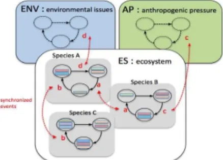
The model we propose is composed of three parts (ES, EN V, AP ) as described in Figure 2. The first part models the dynamics of the ecosystem (ES) itself, that may be composed of elementary interacting models (illustrated, in the figure, as colored rectangles). It describes in a qualitative way the evolution of each entity and the causal influences that exist between them. In our trophic network example, the model is composed of four fish species. The second part models the environmental issues (ENV). It describes the exogeneous constraints, that usually are uncontrollable, but impact, sometimes heavily, the ecosystem. Examples of such environmental drivers are climate evolution or climatic events (e.g. rain, storms, and hurricanes). Some of these can be temporally constrained. For instance, the warming of oceans increases at a (partially) known speed. In our simplified example, we consider only climate change and catastrophic events (hurricanes), that have a strong impact on fish population. The third part models the anthropogenic pressure (AP). It describes the actions that can be decided by humans as resource users or politicians. These events are potentially controllable and impact, in a more or less critical way, the health of the ecosystem. In our case, these actions are fisheries management policies. These three parts of the model interact in a potentially complex way, via shared events (also called synchronized events) and by the clock that is supposed to be shared by the three elements and expresses the temporal constraints.
We first introduce timed automata formalism that is used to represent the qualitative model. Then we present the three parts of our illustrative model. Note that the model has been simplified to serve as a pedagogical tool. A more complicated version is currently beeing developped to look at a coral- reef ecosystem.
2.1
Timed automata formalism
There are many formalisms to represent discrete-event systems, the most common ones being automata theory, statecharts, Petri nets, algebraic approaches, Markov chains and timed automata. In this work, we propose to model the three parts of the qualitative model by timed automata, that were first introduced by Alur and Dill (Alur and Dill 1994). Each component of the system (species, fishing pressures, and environmental constraints) is described as a timed automaton A. Timed automata extend the automata formalism by adding clocks. Clocks are real-valued variables increasing uniformly with time. They define
timing constraints associated with locations (the vertices of the graph) or transitions. In a timed automaton, transitions are instantaneous and allow the resetting of clocks. A timing constraint related to a location is called its invariant. It is possible to stay in a location as long as its invariant is true. A timing constraint related to a transition means that the transition is enabled only when the value of the clocks satisfies the constraint. A clock constraint is the conjunction of atomic constraints which compare the clock value with a non-negative rational.
Timed automata A timed automaton A is a tuple < S, X , L, E, I > where: S is a finite set of locations and so∈ S is the initial location ; X is a finite set of clocks ; L is a finite set of labels ; E is a finite set of edges, each edge e is a tuple (s, l, ϕ, δ, s′) such that e connects the location s ∈ S to the location s′ ∈ S on label l ∈ E, the enabling condition required for all clocks is captured in ϕ and δ ⊆ X gives the set of clocks to be reset when the edge is triggered ; I : S → Φ(X ) maps each location s with a clock constraint called an invariant.
Since it is unrealistic to describe real systems by a single subsystems, the timed automata theory allows the definition of it as a product of its components descriptions. The behavior of the global system is then obtained by the parallel composition of several automata that are synchronized through the label of the edges. When defining an automaton, it is then necessary to distinguish internal events and synchronized events. When a synchronized event is triggered, all subsystems evolve simultaneously. Internal events correspond to asynchronous evolution of the component.
2.2
The anthropogenic pressure (AP) : fishing model
As defined in our trophic network, two fishing pressures are applied on the system. Both follow the same behavior. The automaton, represented in the left of the Figure 3, defines this behavior for the fishing pressure PP0 applied on Species0. A similar one is defined for PP1. Four qualitative strengths of fishing pressure are possible: PP0high, PP0medium, PP0low, PP0null. The evolution between them is gradual except for the cancellation of the fishing pressure (PP0null) that can be applied from any state of the automaton. All the events are synchronized events, since they impact directly on the automaton describing Species0. For example, the event PP0high indicates that the fishing pressure evolves from the medium qualitative state (PP0medium) to the high one (PP0high). PP0high, PP0medium1, PP0low1 are increasing fishing pressure events while PP0medium2, PP0low, PP0null are decreasing fishing pressure events. The automaton described here is a general one in order to describe, in an exhaustive way, the ecosystem automata with regards to the fisheries. For each type of interest problem, more specific fishing pressure can be expressed by adding timing constraints.
Figure 3: Fishing pressure and environmental context automata
2.3
The environmental context (ENV) : climate evolution and environmental
catastrophic events model
The environmental context is described by two automata (see the right of the Figure 3), the first one is related to the disaster, the second one to the ocean warming. Initial states correspond to a situation without any problems. Disaster and warm events are synchronized events. Disaster impacts directly on Species2 and, by regulation, on Species1 and Species3, and warm event impacts on Species3. The ocean warming automaton contains a clock V that is set in the initial state and specifies that the warming occurs after 100 time units.
2.4
The ecosystem dynamics (ES) : fish population dynamics model
The ecosystem dynamics is represented by four automata, each of which is associated with a species in the trophic network. The principles of the approach are explained for Species0 and Species1 automata. For
each species, the automaton describes the evolution of the biomass, defined by qualitative values (Low BM, Medium BM, High BM, Endanger BM) corresponding to an interval of biomass values expressed in g/m2. Each state is associated with a property related to the biomass quantity. For example, in Figure 4, SP 0 M edium BM expresses that the biomass property for Species0 is medium. This biomass property is the only property for equilibrium states (yellow boxes) while for transition states (white boxes), informa-tion about the evoluinforma-tion speed is added (”slow” -one arrow- or ”fast” -two arrows-). Each automaton is associated with a clock : X for Species0 and Y for Species1.
Let us now describe the interaction between the fishing pressure P P 0 and the species Species0 and suppose that the initial biomass for the species is M edium BM . When the fishing pressure increases from PP0medium to PP0high, the event PP0high is triggered. Since this event is synchronized with Species0, the Species0 model goes from state0 to state1 and the clock X is reset. Species0 may stay in this state until X reaches 15 time units, but as soon as X is equal to 12, it may also move to state2, where the biomass value is low. When the automaton of Species0 reaches a state with a new biomass value, a a − kind event (alow, amedium1, ahigh, etc.), denoting a change in the biomass flow between Species0 and Species1, is triggered. So, when Species0 reaches state2, an alow event is triggered and, due to the synchronization with Species1, prey of Species0, it will have an impact on the evolution of Species1.
In the Species0 automaton, only fishing pressure events impact on the evolution of the biomass states. The Species1 automaton is more complicated since it interacts with P P 1 (fishing pressure on Species1), Species0 (its predator), Species2 and Species3 (its prey). When the biomass of Species0 decreases through the event alow, if Species1 is in its initial state, the system moves to state6 indicating that the biomass of Species1 begins to increase. When the automaton of Species1 reaches a state with a new biomass value, a b − kind event (bhigh, bmedium2, bdanger, etc.), denoting a change in the biomass flow between Species1, Species2 and Species3, is triggered. So, due to synchronization constraints, this will have an impact on the evolution of Species2 and Species3, both prey of Species1.
From an environmental point of view, whereas the disaster event causes an immediate change for Species2 into the state Endanger, it causes Species1 to move into a fast decreasing transition state, due to bottom-up regulation.
Figure 4: Species0 and Species1 automata
3
Different types of scenarios
We consider in this section different types of scenarios a user may be willing to explore. We use the term ”‘scenario”’ for denoting a high-level description of a problem. Generally, it means specifying three main issues : i) restricting the general framework by adding a set of constraints that describe a specific situation of interest; ii) giving the temporal window of interest; and iii) expressing the kind of expected answers. In the following, we list a set of scenario frames, that we think are representative of the kind of problems users will want to express. These systems can be classified into two main kinds of queries. The first one are the so-called predictive scenarios, corresponding to ”Given an initial situation and policies, what happens ?” queries, where the difficulties rely in evaluating the complex temporal interactions of each ecosystem submodel, when the ecosystem is subject to environmental and anthropogenic changes. The second are the so-called proactive scenarios, corresponding to ”What to change is needed to reach a specific situation?” queries, that can also be written as ”Which policies to apply to get achieve an objective?”. The concept is to get an idea of the impact of anthropogenic pressure on ecosystem-environment pair. We illustrate each of these cases in our fish population domain. First two are clearly predictive scenarios, the next two are more robustness checking scenarios, and the last one is a proactive scenario.
• The first scenario corresponds to the following issue: ”Given a policy, what will happen on the ecosystem in the near future, depending on the possible occurrence of environmental events?”. More precisely, it is: given E and an ecosystem initial situation described by a set of initial states ei in E, given EN V and a set of initial states envi in EN V and given AP and a set of initial states api in AP , which final states of E will be reached at the end of a given temporal window? See Scenario 1 corresponding to ”What will be the biomass level of the 4 fish species, in 35 time units (let us say months), in the case where the fishing pressure changes from medium to weak for Species0 the next 15 months?”
• The second predictive one is ”Given a policy, is it possible to reach a given state for a given entity? Does it depend on the occurrence of some environmental events? which ones? at which dates?”. On our illustrative example, the query can be: ”Is the fish species Species3 going to be in a dangerous state (i.e. with a low biomass level) if the current policy is not changed, even if i do not consider the risk of a catastrophic climatic event (e.g. hurricane) in the near future?
• The third case considers the impact of environmental events on the ecosystem. As the environmental events are difficult to preview, these scenarios evaluate the robustness of an ecosystem with respect to the climatic events. ”‘Given the current policies and the current situation, what will be, at time t, the impact on the entities of the ecosystem if a specific climatic event occurs at a date t′< t”’. Or ”Is it sure that this risky state will never be reached even if such climatic event occurs? ”.
• An interesting case is when you want to detect whether there exists cases in which you will never be able to jump out from a risky (from an ecological point of view) state, because it is too late to react, or because there is no way to improve the current state.
• A proactive scenario consists in specifying the environmental model EN V and the ecosystem model ES, and looking for policies well-suited to fulfill a specific goal (for instance a satisfying situation). For example, where you are looking for a policy (fishing pressure on Species1 for instance) that will avoid dangerous states, in case of a possible disaster in the next few months.
It can be noted that, even in the simplified example we use for illustration, these kinds of scenarios cannot be answered by only looking at the model. The temporal interactions are sufficiently complex to justify a simulation tool in order to get the answers.
In the following section, we show how the first scenario is translated into logic queries. Let us stress that, in our opinion, the user is supposed to iteratively refine his query according to the first results he gets, and explore the situation using all the capacities of the language and of the tool.
4
Scenarios as model-checking queries
4.1
Few words on model-checking
Model-checking is one of the most successful techniques for automatic verification of complex systems (Hen-zinger et al. 1994; Yovine 1998). It consists of a system specification language, a property specification language and efficient algorithms called model-checkers. The model is generally a set of synchronized au-tomata as presented above for our qualitative model. Examples of well-known model-checking tools are KRONOS(Yovine 1997) and UPPAAAL(Larsen et al. 1997). An important issue is the efficiency of the model-checking algorithms which never explicitly represent all the states of the automaton but rely on sym-bolic methods such as Binary Decision Diagrams (BDD) or Difference Bound Matrices (DBM).
Our implementation has been realized using the tool KRONOS (Yovine 1997) in which the properties are expressed using TCTL (Timed Computation Tree Logic). TCTL formulae are defined using the following grammar:
f ::= p | x ∈ I | ¬f | f1∨ f2 | ∃♦If | ∀♦If
where p ∈ F is a property (fluent), X ∈ X is a clock and I is a time interval. Intuitively, ∃♦If means that there is an execution leading to a state where f holds at time t ∈ I and ∀♦If means that every execution goes through a state where f holds at time t ∈ I. Usually a model-checker answers either by yes or exhibits a counter-example. The model-checker Kronos has been extended to return, when a reachability property is satisfied, the sequences of transitions that lead from the initial state(s) to the final state(s).
4.2
Predictive scenario
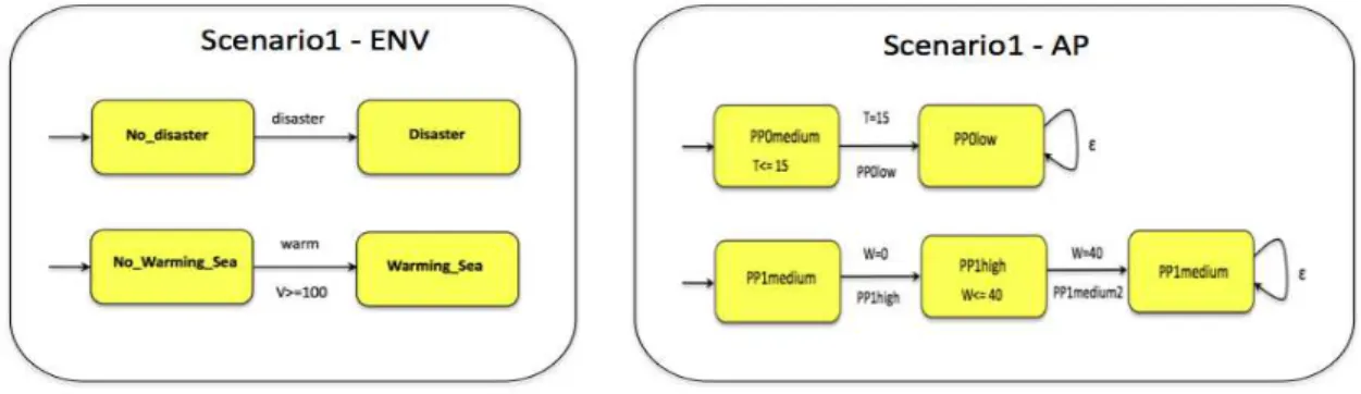
In the case of a predictive scenario, we are interested in the future of the ecosystem, given a specific fishing policy, whatever the environment. To define the scenarios, we firstly have to refine the different parts of the qualitative model (ES, ENV, AP). In the ecosystem, ES, the initial states correspond to the medium biomass for each species. The environmental model is given in its generic form and the occurrence of the disaster is not temporally constrained. The anthropogenic pressure is however clearly known. As can be seen in Figure 5, the fishing pressure on Species0 is medium during 15 time units before becoming low. The fishing pressure on Species1 is initially medium; it moves to high immediatly after and comes back to medium again after 40 time units.
Figure 5: Scenario1 description
4.3
Results
Let us use this scenario in a predictive way to query the model about its evolution after 35 time units and present three variations of queries.
Scenario1: The first query is to predict the qualitative biomasses of each species, after 35 time units, in case no disaster happens. Technically, this query corresponds to a reachability property (i.e does there exist a path from the initial states to specific final states. It is expressed in TCTL as : init ⇒ ∃♦(f inal state ∧ W = 35). The previous formula is submitted to the model-checker Kronos that answers if the reachability property is satisfied or not. The results are the following:
Species0 BM High BM High BM High BM Medium BM Medium BM Medium Species1 BM Endanger BM Low BM Medium BM Medium BM Low BM Endanger Species3 BM Medium BM Medium BM Medium BM Medium BM Medium BM Medium Species4 BM Medium BM Medium BM Medium BM Medium BM Medium BM Medium Result at W=35 possible not possible not possible not possible possible not possible
Result at W=40 possible not possible
Actually only two states are possible at W = 35. Looking to the paths that reach them, it can be easily checked that they correspond to nearly the same trajectories. Due to the time uncertainty on some transition (here the guard 18 ≤ X ≤ 20 associated with the event ahigh of the automaton of Species0), the sequence of events is then : P P 1high ⇒ P P 0low ⇒ blow to reach the final state with the property SP0 BM Medium and SP1 BM Low and P P 1high ⇒ P P 0low ⇒ blow ⇒ ahigh to reach the final state verifying SP0 BM High and SP1 BM Endanger. It is mainly due to the time uncertainty on some transition (here the guard 18 ≤ X ≤ 20 associated to the event ahigh of the automaton of Species0). However, if the user looks at what happens later, for instance at W = 40, it can be checked that only the first state is still possible. It means that the followed fishing policies followed (increasing of P P 1 and, then, at W=15 decreasing of P P 0), causes the biomass of Species1 to decrease from medium to low (blow event) and afterwards the biomass of Species0 to increase. This later change impacts directly on Species1 which already has low resources ; consequently it enters a dangerous situation.
5
Related work and perspectives
Qualitative reasoning techniques started being advocated for dealing with ecological problems in the 90’ when using it like (Guerrin 1991) who used the QSIM simulation tool to look at hydroecology or (Guerrin and Dumas 2001) concerned by the impact of spawning areas on salmon mortality. More recently, more complex models were built, in order to study the interactions of biochemical, physical, chemical processes in marine ecosystems (Salles et al. 2006). Another trend is to study more globally the interactions between environmental, anthropogenic and ecological subsystems as (Tulllos and Neumann 2006) analysing the effects of anthropogenic activities in the watershed on benthic macroinvertebrate communities, and also (Cordier et al. 2005) who propose coupling a biophysical pollutant transfer model and a farm decision-making model to study the impact of agricultural actions (e.g. feeding) on the stream water quality. The main representation used were first purely qualitative representation using directed sign graphs or qualitative algebra (Guerrin 1991). When the dynamic aspects of these systems need to be represented (these aspects corresponding to differential equations in the numerical models), time dating and temporal information had to be introduced (Guerrin and Dumas 2001; Salles et al. 2006). Another way to model the dynamics of an ecosystems is to use finite state machines as automata or more generally discrete-event systems.
Qualitative models and simulations may be useful for understanding the systems and predicting values of variables. However, to fully fulfil their role in a decision-aid context, it is important to propose to the user a powerful, but yet easy way, to express the issues on which they would like to get answers (or at least some help) from the simulation model. For instance, (Attonaty et al. 1999) advocates that models should
be considered as a means to an end, which is to have an interactive debate about a problematic situation in order to decide how to improve it. We fully agree with this ambitious goal and propose to use model-checking techniques on the simulation model as a way to get answers to the user queries. This proposal is close to the work by (Monteiro et al. 2008) for querying qualitative models of genetic regulatory networks. The idea is to propose to users high-level query templates that correspond to frequently-asked questions. These queries are then automatically translated into temporal logic (CTL) expressions.
In this paper, we present an ecosystem modelling to answer predictive scenarios, described with high-level language based on temporal logic. We believe that qualitative models are an efficient tool for marine fisheries management since stakeholder objectives can be associated with scenario templates that can be checked efficiently using model-checking techniques. The refinement of these scenario templates is still in progress. Ongoing work includes the application of this approach on a coral reef ecosystem under fisheries pressure in New-Caledonia. In this larger ecosystem (with roughly ten species and more complicated interactions), the ability to query the model is not only useful in the prediction phase but also during the validation stage. Another interesting perspective is to combine these qualitative models with finer-grained models, and for instance, numerical models. After having a better general understanding of the ecosystem, the user could then focus on a subpart of the model, at a finer resolution. Moreover, up to now, the qualitative ecosystem models have generally been built from expert knowledge and a related bibliography. A challenging future project would be to automatically build these qualitative models by abstracting existing numerical models.
References
Alur, R. and D. Dill (1994). A theory of timed automata. Theoretical computer science 126, pp. 183–235. Attonaty, J. M., M. H. Chatelin, and F. Garcia (1999). Interactive simulation modeling in farm decision
making. Computers and Electronics in Agriculture 22 (2-3), pp. 157–170.
Beaujouan, V., P. Durand, and L. Ruiz (2001). Modelling the effect of the spatial distribution of agricultural practices on nitrogen fluxes in rural catchments. Ecological Modelling 137 (1), pp. 93–105.
Bouyer, P. (2009). Model-checking timed temporal logics. In Proceedings of the 4th Workshop on Methods for Modalities (M4M-5), Volume 231, pp. 323–341. Elsevier Science Publishers.
Cordier, M.-O., F. Garcia, C. Gascuel-Odoux, V. Masson, J. Salmon-Monviola, F. Tortrat, and R. Tr´epos (2005). A machine learning approach for evaluating the impact of land use and management practices on streamwater pollution by pesticides. In MODSIM’05 (International Congress on Modelling and Simulation).
Guerrin, F. (1991). Qualitative reasoning about an ecological process: interpretation in hydroecology. Ecological Modelling 59 (2), pp. 165–201.
Guerrin, F. and J. Dumas (2001). Knowledge representation and qualitative simulation of salmon redd functioning. part i: qualitative modeling and simulation. Biosystems 59 (2), pp. 75–84.
Henzinger, T., X. Nicollin, J. Sifakis, and S. Yovine (1994). Symbolic model checking for real-time systems. Information and Computation 111 (2), pp. 193–244.
Larsen, K., P. Pettersson, and W. Yi (1997). Uppaal in a nutshell. Journal of Software Tools for Technology Transfer 1 (1-2), pp. 134–152.
Monteiro, P. T., D. R. Mateescu, A. T. Freitas, and H. de Jong (2008). Temporal logic patterns for querying qualitative models of genetic regulatory networks. In European Conference in Artificial Intelligence (ECAI’08), pp. 229–233.
Rickel, J. and B. Porter (1997). Automated modeling of complex systems to answer prediction questions. Artificial Intelligence Journal 93, pp. 201–260.
Rykiel, J. (1989). Artificial intelligence and expert systems in ecology and natural resources management. Ecological Modelling 46 (1-2), pp. 3–8.
Salles, P., B. Bredeweg, and S. Arajo (2006). Qualitative models about stream ecosystem recovery: Ex-ploratory studies. Ecological Modelling 194 (1-3), pp. 80–89. Special Issue on the Fourth European Conference on Ecological Modelling - Selected Papers from the Fourth European Conference on Eco-logical Modelling, September 27 - October 1, 2004, Bled, Slovenia.
Tulllos, D. and M. Neumann (2006). A qualitative model for characterizing effects of anthropogenic activ-ities on benthic communactiv-ities. Ecological Modeling 196, pp. 209–220.
Yovine, S. (1997). Kronos : A verification tool for real-time systems (kronos user’s manual release 2.2). International Journal of Software Tools for Technology Transfer 1, pp. 123–133.