HAL Id: hal-01760290
https://hal.archives-ouvertes.fr/hal-01760290
Submitted on 5 Mar 2019HAL is a multi-disciplinary open access archive for the deposit and dissemination of sci-entific research documents, whether they are pub-lished or not. The documents may come from teaching and research institutions in France or abroad, or from public or private research centers.
L’archive ouverte pluridisciplinaire HAL, est destinée au dépôt et à la diffusion de documents scientifiques de niveau recherche, publiés ou non, émanant des établissements d’enseignement et de recherche français ou étrangers, des laboratoires publics ou privés.
Comparaison between two designs of experiment using
the response surface method in order to optimize the
velocity distribution in a coat hanger die
Nadhir Lebaal, Stéphan Puissant, Fabrice Schmidt
To cite this version:
Nadhir Lebaal, Stéphan Puissant, Fabrice Schmidt. Comparaison between two designs of experiment using the response surface method in order to optimize the velocity distribution in a coat hanger die. AMPT 2008 -Advances in Materials and Processing Technologies, Nov 2008, Manama, Bahrain. 20 p. �hal-01760290�
COMPARAISON BETWEEN TWO DESIGNS OF EXPERIMENT USING THE RESPONSE SURFACE METHOD IN ORDER TO OPTIMIZE THE VELOCITY
DISTRIBUTION IN A COAT HANGER DIE N. Lebaal1, S. Puissant1 and F. Schmidt2
1. Institut Supérieur d’ingénierie de la conception, GIP-InSIC (ERMeP), Laboratoire d’Energétique et de Mécanique Théorique et Appliquée (LEMTA), 27 Rue
d’Hellieule, 88100 Saint-Dié, France. ; email: [email protected]
2. Ecole des mines d’Albi Carmaux, CROMeP,- Campus Jarlard- Route de Teillet 81013 Albi Cedex 9, France; email: [email protected]
ABSTRACT
Balancing the distribution of flow through a die to achieve a uniform velocity distribution across the die exit is one of the most difficult tasks of extrusion die design. The objective of this paper is to obtain a homogeneous velocities distribution at the die exit. In order to keep the same geometry and avoid design and manufacture of a new die, it seems very important to control the die thermally. For this, we optimize the wall temperature of regulation of a coat hanger die in a heterogeneous way, (i.e. the wall temperature may not be constant in the entire die). The temperature of regulation of the melt enables us to locally control the viscosity, which influences the flows in the various zones.
The flow analysis results are then combined with an automatic optimisation algorithm that is based on a response surface methodology and a non linear constraint algorithm SQP with several strategies to provide a new profile of the die wall temperature distributions. Two designs of experiment are used and both results are then compared. Typically, for extrusion die design, the objective function states that the average velocity across the die exit is uniform. Constraints are used to limit and /or to control the pressure drop in the die.
KEYWORDS: (Optimization, DoE, Response surface method , FEM)
1. INTRODUCTION
To obtain the optimal parameters during polymer extrusion processes, the numerical simulation imposed itself as an important tool by giving access to difficult orders of magnitudes of physical parameters obtain by the experiment. Moreover it improves the comprehension of the process. Far from being a substitute for the experiment, the numerical simulation allows a time saving and a substantial economy. This is obtained by reducing the number of experiments to be carried out when analyzing the process before its realization. However, obtaining the optimum parameters is often the result of a difficult work of trial and error, during which the various solutions are tested and modified.
The majority of the early works on the extrusion process use the geometrical parameters to optimise the velocity distribution at the die exit [1-4]. The channel geometry of a flat die should be optimized such that a uniform velocity distribution at the die exit is obtained without excessively increasing the pressure drop across the die. Within this framework Smith [5] optimizes a flat die design to well operate at multiple temperatures. The author shows that the
exit velocity distribution is influenced by the melt temperature (the material properties for the power law fluid model are varied according to the melt temperature). To simplify the optimisation approach, the lubrication approximation to model isothermal flow of power-law fluids are used. Design sensitivities needed for the gradient-based constraint optimization algorithm are evaluated with the adjoint variable method to improve the performance and accuracy of the computations.
If the non isothermal flow is not accounted while optimizing the die [6] the computed velocity pressure fields are expected to have large errors [5]. The non-isothermal flow of a power-law fluid in a coat-hanger die is studied by Vergnes et al. [7]. The authors employed the finite difference method to solve the two dimensional equilibrium and thermal equations (flow field by considering the thermal regulation). The pressure, residence time, and temperature distribution are obtained. The authors show that the thermal regulation and temperature dependence of the viscosity have a large effect on the flow uniformity at the end of the die. Schläfli [8] made an experimental study on the effect of the difference of the temperature between the material and the die on the velocity distribution at the exit of a Coat-hanger melt distributors. He noted that the difference in temperature has a more important effect on the final zone of the distribution channel because of the more important residence time. Within the framework, Vergnes et al. [9] were interested in the manufacture of a tube. The problem encountered during this manufacture is the presence in the section of the tube of a symmetrical extra thickness. This defect is due to the existence, in the entry of the die, of two hotter zones of melt due to the flow in the twin screw extrusion machine. These hot zones separate to flow out on each side of the punch, providing, because of their lower viscosity, more important local flows and thus, extra thicknesses at the exit. To obtain a homogeneous distribution of the flow at the die exit, instead of imposing a homogeneous temperature of regulation, they imposed a heterogeneous temperature of regulation compared to the cold and hot zones. The results show that with this heterogeneous wall temperature, they obtained a practically homogeneous distribution of thickness all around the die. This possibility of heterogeneous thermal regulation was applied and exists at the industrial level. Fradette et al. [10] optimize the cooling channels diameter and position for the cooling layout of vacuum calibrators used in the extrusion of PVC profiles. The required objective is to minimize the average temperature to decrease the time of cooling and to standardize the temperatures to improve quality. The methodology is based on the finite element resolution of the heat transfer conduction problem in the calibrator and the profile coupled to the Fletcher-Reeves optimization algorithm.
For complex geometries, the computational resources and time required for analysis of extrusion dies are considerable. Consequently, the use of evolution strategy algorithm to optimize the extrusion die in three-dimensional analysis is less attractive to designers because of the unacceptable turnaround time for results. The purpose of this work is to deal with this inconvenient disadvantage, by using an automatic optimisation algorithm and several strategies which permit to avoid the local minima and by this fact without increasing the computing time which becomes penalizing for three-dimensional simulations. The non isothermal flow analysis results are then combined with an automatic optimisation algorithm that is based on a response surface methodology [11] and a non linear constraint algorithm SQP to optimize the wall temperature profile of a coat hanger die in a heterogeneous way.
To obtain the optimal parameters during polymer extrusion processes, the numerical simulation imposed itself as an important tool by giving access to difficult orders of magnitudes of physical parameters obtain by the experiment. Moreover it improves the comprehension of the process. Far from being a substitute for the experiment, the numerical simulation allows a time saving and a substantial economy. This is obtained by reducing the number of experiments to be
carried out when analyzing the process before its realization. However, obtaining the optimum parameters is often the result of a difficult work of trial and error, during which the various solutions are tested and modified.
The majority of the early works on the extrusion process use the geometrical parameters to optimise the velocity distribution at the die exit [1-4]. The channel geometry of a flat die should be optimized such that a uniform velocity distribution at the die exit is obtained without excessively increasing the pressure drop across the die. Within this framework Smith [5] optimizes a flat die design to well operate at multiple temperatures. The author shows that the exit velocity distribution is influenced by the melt temperature (the material properties for the power law fluid model are varied according to the melt temperature). To simplify the optimisation approach, the lubrication approximation to model isothermal flow of power-law fluids are used. Design sensitivities needed for the gradient-based constraint optimization algorithm are evaluated with the adjoint variable method to improve the performance and accuracy of the computations.
If the non isothermal flow is not accounted while optimizing the die [6] the computed velocity pressure fields are expected to have large errors [5]. The non-isothermal flow of a power-law fluid in a coat-hanger die is studied by Vergnes et al. [7]. The authors employed the finite difference method to solve the two dimensional equilibrium and thermal equations (flow field by considering the thermal regulation). The pressure, residence time, and temperature distribution are obtained. The authors show that the thermal regulation and temperature dependence of the viscosity have a large effect on the flow uniformity at the end of the die. Schläfli [8] made an experimental study on the effect of the difference of the temperature between the material and the die on the velocity distribution at the exit of a Coat-hanger melt distributors. He noted that the difference in temperature has a more important effect on the final zone of the distribution channel because of the more important residence time. Within the framework, Vergnes et al. [9] were interested in the manufacture of a tube. The problem encountered during this manufacture is the presence in the section of the tube of a symmetrical extra thickness. This defect is due to the existence, in the entry of the die, of two hotter zones of melt due to the flow in the twin screw extrusion machine. These hot zones separate to flow out on each side of the punch, providing, because of their lower viscosity, more important local flows and thus, extra thicknesses at the exit. To obtain a homogeneous distribution of the flow at the die exit, instead of imposing a homogeneous temperature of regulation, they imposed a heterogeneous temperature of regulation compared to the cold and hot zones. The results show that with this heterogeneous wall temperature, they obtained a practically homogeneous distribution of thickness all around the die. This possibility of heterogeneous thermal regulation was applied and exists at the industrial level. Fradette et al. [10] optimize the cooling channels diameter and position for the cooling layout of vacuum calibrators used in the extrusion of PVC profiles. The required objective is to minimize the average temperature to decrease the time of cooling and to standardize the temperatures to improve quality. The methodology is based on the finite element resolution of the heat transfer conduction problem in the calibrator and the profile coupled to the Fletcher-Reeves optimization algorithm.
For complex geometries, the computational resources and time required for analysis of extrusion dies are considerable. Consequently, the use of evolution strategy algorithm to optimize the extrusion die in three-dimensional analysis is less attractive to designers because of the unacceptable turnaround time for results. The purpose of this work is to deal with this inconvenient disadvantage, by using an automatic optimisation algorithm and several strategies which permit to avoid the local minima and by this fact without increasing the computing time which becomes penalizing for three-dimensional simulations. The non isothermal flow analysis results are then combined with an automatic optimisation algorithm that is based on a response
surface methodology [11] and a non linear constraint algorithm SQP to optimize the wall temperature profile of a coat hanger die in a heterogeneous way.
2. MESH SIZE SENSITIVE
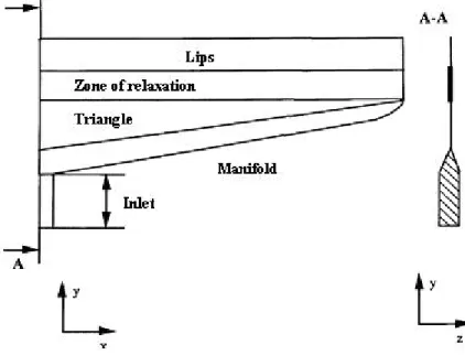
In this section we examine and analyze the effect of the mesh size over CPU time and on some results: pressure in the die entrance, and the exit velocity distribution. The mesh distribution was improved by dividing the die into four zones. The first zone represents the entry of the die and the manifold. The other zones (2, 3, 4) represent the zones of low thickness of the die (land), which are respectively: the triangle, the relaxation zone, and the lips, as figure 1 indicates. On these zones we will impose various sizes of finite elements. Considering the great shape ratio (thickness over width) (fig. 2) and to respect some number of node on the thickness the anisotropic mesh is privileged (i.e. size of element which varies according to each direction). Seven mesh sizes were analyzed. In table 1, we present the characteristics of each mesh: elements size according to each direction and for the various zones, node and element numbers, CPU time and pressure drop in the die.
0 50 100 150 200 250 300 350 400 450 20 30 40 50 60 70 80 90
Largeur de la demi filière [mm]
Vi te s s e [m m /s ] Maillage 1 Maillage 2 Maillage 3 Maillage 4 Maillage 5 Maillage 6 Maillage 7
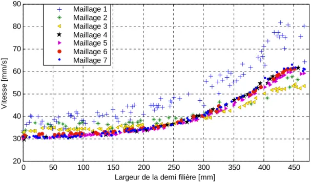
Figure 2. Mesh size effects on the exit velocity distribution.
We compare the pressure obtained by the various mesh size with that obtained by the finest mesh taken as reference. Thus, we note, according to the results obtained (table .1), that by refining the mesh and by using an adapted mesh for each zone, the difference between the pressures becomes negligible; on the other hand, the CPU time becomes more important.
In order to quantify the influence of the mesh density on the exit velocities distribution, we represent in figure .2 the results corresponding to the various mesh size.
Tableau 1. Characteristics of the various mesh size
Mesh size [ mm ] according to each direction for the various zones
Zone 1 Zone 2 Zone 3 Zone 4 Mesh x y z x y z x y z x y z Nodes Elements Pressure [MPa] CPU Time [min] (1) 4 4 4 2 2 2 2 2 2 1 1 1 135357 659761 4.87 267 (2) 6 3 7 6 1.5 6 6 1.5 6 5 1 5 20708 94113 3.95 14 (3) 6 4 6 6 1 6 6 1.5 6 3 0.75 3 24380 112209 3.98 26 (4) 6 4 6 4 0.75 4 5 1 5 3 0.5 3 35837 176806 4.44 49 (5) 5 2 5 4 0.75 4 4 1 4 3 0.5 3 60356 302588 4.43 85 (6) 4 1 4 2 0.5 2 2 0.5 2 2 0.37 2 104208 532018 4.48 192 Reference (7) 2 1 2 1 0.37 1 1 0.37 1 1 0.37 1 220888 1146689 4.46 431
We note that the exit velocities distribution converge by refining the mesh with very close values. By analyzing more closely the curves, we remark that a stabilization of the results is established starting from mesh 4.
3. OPTIMISATION PROCEDURE
3.1 Optimization variables
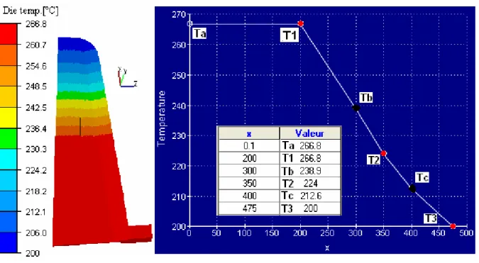
In order to keep the same geometry and obtain a homogeneous velocity distribution at the die exit, an optimization problem is formulated, which consists in optimizing the temperature of regulation of the flat die. For this procedure, the geometry of the die as well as the mesh remains constant. On the other hand, physical parameters, which represent the wall die temperatures of regulation, will be used as optimization variables to obtain a homogeneous exit velocity distribution. 6 temperatures of regulation "T1, T2, T3, Ta, Tb and Tc" are imposed according to the width of the die (Fig.1). Because of symmetry, we represented only half die. To decrease the number of optimization variables, we use a control curve obtained by Kriging, to allow the control of the die wall temperature profile, and to decrease the number of variables to 3.
Among the 6 optimization variables Ta, Tb and Tc are active; whereas, T1, T2, and T3 are passive. This means that T1 varies like Ta, at the distance from 0 to 200 mm of the width of the die. From the three temperatures (active variables), we can plot a curve using the Kriging interpolation to represent other die wall regulation temperatures (passive variables). The other temperatures T2 and T3 are determined according to Ta, Tb, Tc according to the curve of Kriging interpolation.
Figure 3. Wall temperatures distribution according to the width of the die (optimization variables).
The optimization problem is thus resolved with three parameters (Ta, Tb, and Tc). We can also add to it the applied constraint conditions so that the temperatures do not exceed a certain value. Initially, the temperature of regulation is constant through all the width of the die T=230°C. This constant temperature gives a non uniform velocity distribution. Velocities are more important of about 50% at the edge and weaker of about 25 % in the middle of the die compared to the average velocity. During the optimisation processes the variables permit the variation between 200°C and 280 °C. The maximum temperature of 280°C is chosen i.e. there is no polymer degradation.
3.2 Objective and constraint Function
The problem consists in determining the optimal profile of wall temperatures of this coat hanger die so that the objective function based on the exit velocity distribution is minimal; the sheet thickness will be then homogeneous. This represents a very important material profit considering the quantity of the extruded polymer sheets each year. The objective function ( f
( )
x ) represents the total relative variation on the exit velocity distribution. In order to ensure that the pressure at the entry of the die ( eP ) does not increase compared to the pressure obtained by the initial wall temperature ( e
P0 ), a constraint function (g
( )
x ) based on the pressure at the entry of the die is used. This problem of optimization is represented by the equation (1).( )
( )
⎪ ⎪ ⎪ ⎩ ⎪ ⎪ ⎪ ⎨ ⎧ ≤ ≤ ≤ − = = max min 0 0 0 0 min x x x P P P x g E E x f e e e (1)The velocity dispersion ( E ), is defined as: ⎟ ⎟ ⎠ ⎞ ⎜ ⎜ ⎝ ⎛ ⎟⎟ ⎠ ⎞ ⎜⎜ ⎝ ⎛ − =
∑
N= i i v v v N E 1 1 (2) whereE and 0 P are respectively the total relative variation of the exit velocity distribution 0and the pressure in the initial die, N is the total number of nodes at the die exit in the middle plane; v is the velocity at an exit node, and v is the average exit velocity which is defined as i follows:
∑
= = N i i v N v 1 1 (3) minx and xmax are the lower and higher limits of optimization variables, with:
⎪ ⎭ ⎪ ⎬ ⎫ ⎪ ⎩ ⎪ ⎨ ⎧ ° = ° = ° = = C Tc C Tb C Ta x 200 200 200 min min min min et ⎪ ⎭ ⎪ ⎬ ⎫ ⎪ ⎩ ⎪ ⎨ ⎧ ° = ° = ° = = C Tc C Tb C Ta x 280 280 280 max max max max (4)
The maximum temperature of 280°C is chosen so there is no polymer degradation. 3.3 Sensitive analysis
A Taguchi method [12] is used to investigate the sensitive analysis effect of the optimization variables (regulation temperature) in the objective and constraint function. The central composite design or CCD is the most popular class of designs used for fitting a second-order model. The CCD consists of a 2k factorial with runs, 2 k axial or star runs, and central runs. The parameter, which represents the distance of the axial runs from the design centre must be specified.
The rotatability is important for the second–order-model to provide good predictions throughout the region of interest. One way to well define is to require that the model have a
reasonably consistent and stable variance of the predicted response at point of interest. Because the purpose of RSM is the optimization and location of the optimum prior to running the experiment, is important to use a design that provides equal precision of estimation in all directions. For this, the CCD is made rotatable.
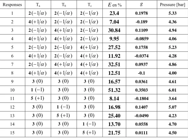
In this first study, in order to evaluate the effects of the optimization variables on the objective and constraint function, Taguchi design of experiments method was used to estimate the effects of the profile of the die wall temperature on the pressure drop and on the exit velocities distribution and to identify the influential parameters. This method uses a central composite design (CCD) [12], to study the entire parameter space with only small number of experiments. In this study, three parameters were considered with five levels each. According to the Taguchi quality design concept, 15 complete simulations were chosen. The various levels are represented from 1 to 5 respectively giving the values of the minimum to the maximum of each variable. For this, we have calculated the effect of each variable over all the field of research by studying the contribution of each variable on the variation of the response “objective and constraint function " (Table 2).
Table . 2. Response of the objective and constraint functions using CCD.
Responses Ta Tb Tc Een % g Pressure [bar]
1 2(−1α) 2(−1α) 2(−1α) 23.4 0.1978 5.33 2 4(+1α) 2(−1α) 2(−1α) 7.04 -0.189 4.36 3 2(−1α) 4(+1α) 2(−1α) 30.84 0.1109 4.94 4 4(+1α) 4(+1α) 2(−1α) 9.95 -0.0859 4.06 5 2(−1α) 2(−1α) 4(+1α) 27.52 0.1758 5.23 6 4(+1α) 2(−1α) 4(+1α) 11.92 -0.0374 4.28 7 2(−1α) 4(+1α) 4(+1α) 32.51 0.0937 4.86 8 4(+1α) 4(+1α) 4(+1α) 12.51 -0.1 4.00 9 3 (0) 3 (0) 3 (0) 16.57 0.0361 4.61 10 1 (−1) 3 (0) 3 (0) 51.32 0.3503 6.01 11 5 (+1) 3 (0) 3 (0) 8.14 -0.1804 3.64 12 3 (0) 1 (−1) 3 (0) 16.98 0.1407 5.07 13 3 (0) 5 (+1) 3 (0) 25.40 -0.0490 4.23 14 3 (0) 3 (0) 1 (−1) 13.70 0.0558 4.70 15 3 (0) 3 (0) 5 (+1) 21.75 0.0111 4.50
The average effects of the various variables are represented on graphs to support the discussion and to lead to the identification of those influencing to minimize the defects.
Ta1 Ta2 Ta3 Ta4 Ta5 Tb1 Tb2 Tb3 Tb4 Tb5 Tc1 Tc2 Tc3 Tc4 Tc5 -0.2 -0.1 0 0.1 0.2 0.3
Parameters with levels
A v e ra g e ef fe c t o n t he ob je c ti v e f unc ti o n Ta Tb Tc
Figure 4. Average effect of variables levels on the objective function (exit velocity distribution).
Figure 4 represent the average effect of the optimization variables on the objective function (velocities distribution at the die exit). It is noted that the temperature Ta have a most important effect on the velocities distribution. This temperature is located at the medium of the die, where the velocities are lowest. For the other temperatures, Tb and Tc seem having less important effects. We notice that the combination which offers the minimum of the objective function, corresponds to the maximum of the temperature Ta, and the minimum of the temperatures Tb, and Tc. This allows to change the polymer viscosity and control the flow locally. At this place, or the air-gap is weaker, that compensates for the lack of flow on this zone. On the other hand, for the zones located on the edge of the die (more important velocities), the temperatures of regulation Tb and Tc, which are low, generate an increase in viscosity, and thus a reduction in the flow.
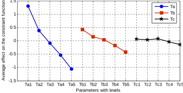
Ta1 Ta2 Ta3 Ta4 Ta5 Tb1 Tb2 Tb3 Tb4 Tb5 Tc1 Tc2 Tc3 Tc4 Tc5 -1.5 -1 -0.5 0 0.5 1 1.5
Parameters with levels
A v e rag e e ff e c t on t h e c o ns tr ai nt f u nc ti o n Ta Tb Tc
Figure 5. Average effect of variables levels on the constraint function (pressure).
Concerning their effects on the pressure (fig.5) we can classify them by descending order. The greatest effect on the pressure variation is given by Ta, then Tb and finally Tc which has the weakest effect. The combination, of the optimization variables, which offers the minimum of the
constraint function (pressure), corresponds to the maximum of the temperatures of regulation. That makes it possible to increase the melt temperature. Into consequent, the melt viscosity decreases, which favourite the flow with less pressure loss.
3.4. Response surface method
The objective and constraint functions are implicit, compared to the optimization parameters and their evaluation requires a large amount of computing time using three dimensional analyses. In order to decrease the evaluation number of the objective and constraint functions we use in this work the response surface method [11, 13] which consists in the construction of an approximate expression of the objective and constraint functions starting from a limited number of evaluations of the real function. In order to obtain a good approximation, we used a Kriging interpolation described in next section. In this method, the approximation is computed by using the evaluation points obtained using Design of Experiments technique.
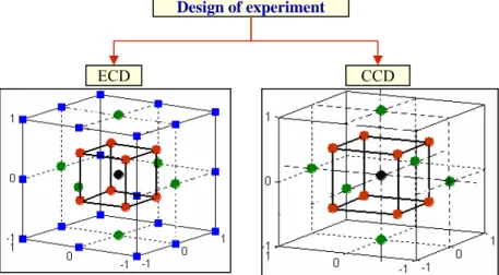
Two optimization results are built (conducted) using two DoE for the construction of the R.S (figure 6) the firs one is the Enriched Composite Design (ECD) and the second is the Central Composite Design (CCD).
Figure 6. Design of experiment.
3.5. Kriging interpolation
Kriging is an interpolation technique [14, 15] which allows to model very efficiently complex functions. It is applied here to represent the response surface in an explicit form, according to the variables of optimization. The explicit relationship of the objective and constraint function can be expressed as follows: Z(x) a (x) p (x) J~ = T + (5) with,
( )
( )
T m x p , , x pp(x)=[ 1 K ] , where m denotes the number of the basis function in
regression model, T m ] a , , a [
a= 1 K is the coefficient vector the, x is the design variables, (x)
J~ is the unknown objective or constraint interpolate function, and Z(x) is the random fluctuation. The term pT(x)a in Equation (5) indicates a global model of the design space, which is similar to the polynomial model in a Moving Least Squares (MLS) approximation. The second
Design of experiment
CCD ECD
part in Equation (5) is a correction of the global model. It is used to model the deviation from a
(x)
pT so that the whole model interpolates response data from the function. The output responses from the function are given as:
( ) ( )
( )
{
f x f x f x}
xF( )= 1 , 2 ,K n (6)
From these outputs the unknown parameters a can be estimated: F R P P) R (P a= T −1 −1 T −1 (7)
Where P is a vector including the value of p(x) evaluated at each of the design variables and R is the correlation matrix, which is composed of the correlation function evaluated at each possible combination of the points of design:
(
)
(
)
(
)
(
)
(
)
(
)
(
)
⎥⎥ ⎥ ⎥ ⎦ ⎤ ⎢ ⎢ ⎢ ⎢ ⎣ ⎡ − − − + ⎥ ⎥ ⎥ ⎦ ⎤ ⎢ ⎢ ⎢ ⎣ ⎡ = n 2 1 n n 1 n n 1 1 1 0 0 0 0 0 0 x , x , x , x , x x w x x w x x w x R x R x R x R R L M M M M L L L M O M L (8)(
)
3 j i j i x x R = − (9)A weight function of Gaussian type with a circular support is adopted for the Kriging interpolation because its derivatives with respect to the coordinates exist to any desired order. It takes the form
⎪⎩ ⎪ ⎨ ⎧ ≥ ≤ ⎟⎟ ⎠ ⎞ ⎜⎜ ⎝ ⎛ − − − − − − = w i w i w w i i r d r d c r c r c d x W χ χ * ) ) / ( exp( 1 ) ) / ( exp( ) ) / ( exp( 1 ) ( 2 2 2 (10) where
(
())
2 1 i J J n J i x x d =∑
− =is the distance from a discrete node x to a sampling point x i in the domain of support with radius r , and c is the dilation parameter. w
4
w
r
c= is used in computation. 0≤χ ≤1 represents the degree of the importance of the weight function.
The second part in Equation (5) is in fact an interpolation of the residuals of the regression modelpT(x)a. Thus, all response data will be exactly predicted; is given as:
( )
x r( )β
xZ = T (11)
Where rT
( )
x ={
R(
x,x1)
,L,R(
x,xn)
}
The parameters β are defined as fallow:(
F Pa)
R −
= −1
β (12)
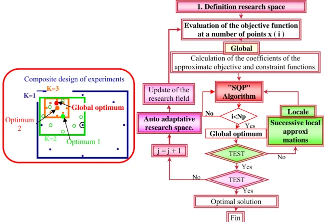
3.6.Optimization strategy
In order to reach a true global optimum (defined by the exact response) and to respect the non linear constraint function, an efficient optimization strategy using response surfaces are build:
In the first step we use the global response surface, using the DoE defined on the whole research space. The objective and constraint functions will be computed into a limited evaluation response, and we minimize it using a SQP (sequential quadratic programming method). To avoid local minima, and by this fact without increasing the computing time which becomes penalizing for three-dimensional simulations we change the initial points of the SQP method by all the points of the DoE because the evaluation of the explicit functions does not cause problems and does not take much time. When we have obtained the best minimum; successive local approximate problems based on the weight function of Gaussian type are then solved using an SQP algorithm. This weight function gives, also more importance to the responses which are closer to the minimum and less importance to the other responses, which allows makes the response surface more accurate locally.
During the progression of the optimization procedure (figure 7), the region of interest moves and zooms on each optimum by reducing the search space by 1/3. In addition,
We enriches then the collection { k
x } with the points by the vicinity ℜxmink . Giving a new collect
{ } { }
k k xk xx +1 = ∪ℜmin at the stage k+1 . At this iteration ( k+1 ) we construct a new approximation ~k+1
f starting from {xk+1}. The number of evaluation points considered increases because of enriching the collection { k
x } with the points by the vicinity. This carries out to an auto adaptive search space and increases the accuracy when we approach the optimum. These steps are repeated till the new profile temperature satisfies the objective and the constraints function and the iterative procedure stops when the successive points are superposed with a tolerance of ε=10-3.
Figure 7. The flowchart of the adopted optimization strategy.
Evaluation of the objective function at a number of points x ( i ) 1. Definition research space
No
"SQP" Algorithm
Calculation of the coefficients of the approximate objective and constraint functions.
TEST Successive local approxi mations Global optimum i<Np No Yes Locale Global
Composite design of experiments K=1 K=3 Optimum 1 K=2 Optimum 2 Global optimum Yes Yes Update of the research field TEST No Optimal solution j = j + 1 Fin Auto adaptative research space.
4. NUMERICAL APPLICATION
The optimization strategy applied consists in using the optimization algorithm described previously, based on the response surfaces method and the Kriging interpolation. Two results are presented by using two different experimental designs:
• Case 1: Optimization is carried out by using an Enriched Composite Design of experiment (ECD).
• Case 2: We a Central Composite Design of experiment (CCD).
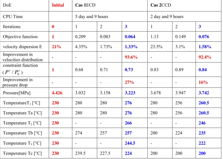
The process of optimization is carried out and the obtimum is obtained from the 3rd iteration; therefore a very fast convergence is obtained for the two results. These calculations take a computing CPU time of 5 days and 9 hour for the ECDs and 2 days and 9 hours for the CCD on a machine Pentium IV, 3 GHz, 1 Go RAM.
The results for the objective function (velocities distribution at the die exit) and the constraint function (pressure) are normalised (standardized) compared to the results obtained with the same geometry by imposing a constant wall temperature over all the width of the die (Tw=230°C). A
first observation in table 3 shows that with the two results, we find very satisfactory solutions, and that the value of the cost function is reduced moreover than 92%. The constraints on the pressure are respected for the two solutions, as well as the velocities distribution is better. The optimal solution is obtained after three iterations for the two results. On the other hand, the computing time is more important by using the enriched composite design (ECD) (cas1). With the use of the CCD (cas2), we can obtain a reduction of CPU time of about 66%. The optimum parameters obtained are given in table 3.
Table 3. Summary of the results for the two optimization cases.
DoE Initial Cas 1ECD Cas 2CCD
CPU Time 5 day and 9 hours 2 day and 9 hours
Iterations 0 1 2 3 1 2 3 Objective function 1 0.209 0.083 0.064 1.13 0.149 0.076 velocity dispersion E 21% 4.35% 1.73% 1.33% 23.5% 3.1% 1.58% Improvement in velocities distribution - - - 93.6% - - 92.4% constraint function ( e e P P / 0 ) 1 0.68 0.71 0.73 0.83 0.89 0.84 Improvement in pressure drop - - - 27% - - 16% Pressure[MPa] 4.426 3.032 3.158 3.223 3.678 3.947 3.742 TemperatureT1 [°C] 230 280 280 276 280 256 260.5 Temperature Ta [°C] 230 280 280 276 280 256 260.5 Temperature T2 [°C] 230 - - 266 - - 246 Temperature Tb [°C] 230 274 257 257 200 224 235 Temperature T3 [°C] 230 - - 244.5 - - 222 Temperature Tc [°C] 230 239.5 227.5 224 200 200 200
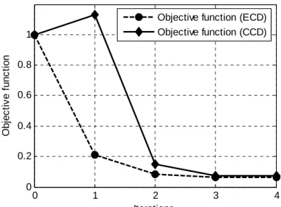
0 1 2 3 4 0 0.2 0.4 0.6 0.8 1 Iterations O b je c ti v e fu n c ti o n
Objective function (ECD) Objective function (CCD)
Figure 8. Convergence history during an optimization process on the objective functions.
The figure 8 represents the evolution of the objectives functions (E/E0) for the two optimization results (cas1 and cas2). We note that with the use of the ECD we obtain a reduction of 80% of the objective function at the first iteration, since the good interpolation obtained by Kriging. At the second and third iteration, the objective function decreases gradually until obtaining a profit of homogeneity of 93.5% compared to the exit velocities distribution obtained initially.
With the use of the CCD, the solution (total relative variation) obtained at the first iteration is higher than the initial solution obtained with a constant wall temperature. This is due to the weak evaluation points for the field of research which varies between 200 and 280°C, which makes the approximation less accurate. On the other hand, at the second iteration, the objective function decreases by 85%, then of 92.4% with the third iteration. The strategy of auto-adaptive search space makes it possible to enrich the approximation and to make it more accurate when we approach the global optimum.
0 50 100 150 200 250 300 350 400 450 0 10 20 30 40 50
Width of half die [mm]
R e la ti ve ve lo c ity va ri a ti o n %
Initial wall temperature
Optimal wall temperature using (ECD) Optimal wall temperature using (CCD)
Figure 9. Relative variation of the exit velocities distribution with initial and optimal wall die temperature distribution using (ECD & CCD) .
The figure 9 represents the relative variation of the exit velocities distribution obtained in the initial die wall temperature of regulation and after optimization for both results (using two design of experiment). Qualitatively it is clear that the velocities distribution obtained with the initial temperature (T= 230°C) gives more important relative variations, about 25% in the middle of the die and 50% at the edge. This important relative variation, result in lower velocities in the middle of the die, and more important velocities distribution on the edge. After optimization, we note that the velocities distribution is homogeneous over all the width of the die exit. The relative variations are lower than 5 % over all the width of the die.
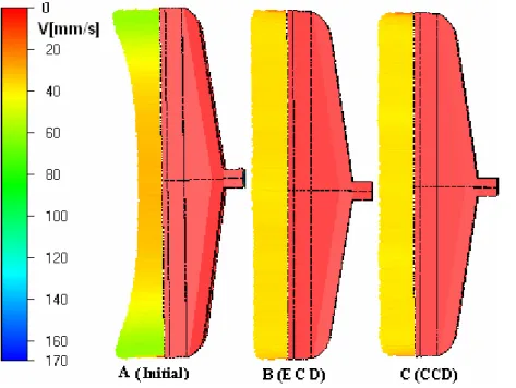
Figure 10. Exit velocity distributions in the initial (A), and optimized (B,C) temperature of regulation.
Qualitatively we find that the initial wall die temperature of regulation (Fig.10- A) gives a not homogeneous velocities distribution. The optimal solution obtained for two optimizations using ECD and CCD (B and C), represents hotter temperatures of regulation in the middle of the die. The local flows are more important there and a compensation of the flow diminution is thus obtained compared to the initial regulation. On the other hand, the temperatures are lower on the edge to increase the polymer viscosity. This generates a reduction in the flow towards the edge. With these optimal temperatures of regulation, we could obtain a balance which makes it possible to give a homogeneous exit velocities distribution according to all the width on the die (Fig.10 B and C).
0 1 2 3 4 0.65 0.7 0.75 0.8 0.85 0.9 0.95 1 Iterations C o n s tr a in t fu n c ti o n ( P /P 0 ) [P/P0] ECD [P/P0] CCD
Figure 11. Convergence history during an optimization process on the constraint functions.
The figure 11 shows that the constraint on the pressure is respected for the two results (ECD and CCD). This constraint represents the ratio the pressure, in each iteration, and the pressure obtained with the initial temperature of regulation ( e e
P
P / 0 ). The optimization problem was formulated so that the ratio ( e e
P
P / 0 ) remains lower than 1 for each iteration, which gives a pressure decrease. We notes according to the constraints evolution according to the optimization iterations, that we obtains a profit of pressure of about 27% with the 3rd iteration for the ECD (cas1). On the other hand, the pressure profit obtained by using a CCD (cas2) is lower, it accounts for 15% compared to the initial pressure.
Figure 12. Pressure distributions in the initial (a), and optimized (b,c) temperature of regulation.
The pressure drop in the initial wall die temperature of regulation was specified as the limit pressure drop in the optimization algorithm. The goal was to improve the uniformity of exit velocity without increasing the pressure drop in the die. We show in the figure 12, that the pressure drop in the coat-hanger die, is lower for the two results (B, and C). The optimal temperatures of regulation obtained by using the EDC (A) are higher. This made decrease the viscosity of polymer and thus implies a weaker pressure drop (see the study of the effect of the optimization variables on the pressure figure 5). The pressure is decreased by 27%, compared to the limit pressure drop obtained by initial temperature of regulation. On the other hand, the temperatures of regulation obtained by using CCD (C) are lower compared to the result (B). This decrease the pressure drop by 16%.
Figure 13. Convergence history during an optimization process on the optimizations variables.
The graph (Fig.13) represents the evolution of the optimization variables (temperatures of regulation) during iterations of optimization. The solutions of the two results are different; on the other hand they have the same gradient. It is noted that the wall temperatures of regulation obtained by the first optimization (cas1) are higher. The temperature in the middle of the die (Ta)
is about 276°C, then it decrease according to the width of the die as illustrated on the figure 14 until the lowest temperature at the edge of the die Tc, which is equal to 223.5°C. It is noted that the difference of temperatures between «Ta, Tb» and «Tb, Tc», is respectively 19°C and 33°C.
0 1 2 3 4 200 220 240 260 280 Iterations T e m p e rat ur e s [ °C ] T a Tb T c 0 1 2 3 4 220 230 240 250 260 270 280 Iterations T e m p era tures [ °C ] Ta Tb Tc (ECD) (CCD)
Figure 14. Distribution profile of optimal regulation temperature (ECD).
Figure 15. Distribution profile of optimal regulation temperature (CCD)
For Cas2, we notice that the temperatures are lower (fig. 15). On the other hand, the differences in temperature between the various zones are a little stronger. These differences represent 25°C and 35°C respectively between the temperatures "Ta Tb" and between "Tb Tc"
Figure 16. Temperature distributions in the mid-plane of the initial (a), and optimized (b,c) temperature of regulation of the flat die.
The figure 16 illustrates the Temperature distributions in the mid-plane of the initial (a), and optimized (b,c) temperature of regulation of the flat die. It is noted that for the temperature of initial regulation (constant wall die temperature), the melt temperature is higher on the edge and less low in the middle of the die. This difference in temperature which remains low ( ∆Tinitiale =3°C ), be essential caused by viscous dissipation. However, we note that the difference in melt temperature obtained by the optimal wall die temperatures of regulation is more important according to the width of the die, because of the imposed temperatures of regulation. The difference in temperature is of 10°C for two optimizations (∆TB ≈∆TC ≈10°C).This difference in temperature can generate difficulties during drawing and cooling on the outlet side of the die.
5. CONCLUSION
In this paper, a procedure was applied in order to optimize the distribution of temperatures of regulation of a coat hanger die. The optimisation method is based on a Surface Response Method and has a very fast convergence, which is an advantage when time-consuming flow analysis calculations are involved.
The advantage of such an approach lies in its (adjustment) facilitated of implementation to geometrical optimization. A curve of control was introduced in order to decrease the number of variables to 3 while keeping 6 temperatures of regulation. Two optimization cases were carried out according to the used experimental design. The two results show an improvement of the velocity distribution higher than 92% compared to the reference solution. The taking into account of the nonlinear constraint allowed decreasing the pressure at the end of the optimization. Nevertheless, the weakness lies in the difference of the temperatures on the outlet side of the die. This is likely to generate difficulties during the operations of drawing and cooling. In the continuation we will optimize the geometry of a cylindrical die and will carry out experimental validations.
6. BIBLIOGRAPHY
[1] J. M. Nóbrega, O. S.Carneiro, F. T.Pinho, P. J.Oliveira, Flow Balancing in extrusion dies for thermoplastic profiles, Int. Polym. Process. 19 (2004) 225-235.
[2] H. J.Ettinger, J.Sienz, J. F. T. Pittman, A. Polynkin, Parameterization and optimisation strategies for the automated design of U PVC profile extrusion dies. Struct. Multidisc. Optim. 28 (2004) 180-194.
[3] W. Michaeli, S. Kaul, T. Wolff, Computer aided optimisation of extrusion dies, J. Polym. Eng. 21 (2001) 225-237.
[4]. Y. Sun, M. Gupta, Optimization of a flat die geometry, SPE ANTEC Tech. Papers, (2004) 3307-3311.
[5] D.E. Smith, An optimisation-based approach to compute sheeting die designs for multiple operating conditions, SPE ANTEC Tech. Papers, (2003) 315-319.
[6] Y. Wang, The flow distribution of molten polymers in slit dies and coat hanger die through three-dimensional finite element analysis, Polym. Eng. Sci. 31 (1991) 204-212.
[7] B. Vergnes, P. Saillard, J.F. Agassant, Non-isothermal flow of a molten polymer in a coat-hanger die, Polym. Eng. Science 24 (12), pp. 980-987 1984
[8] D. Schläfli, Analysis of polymer flow through coat-hanger melt distributors, Int. Polym. Process., 10 (1995) 195.
[9] B. Vergnes, J.F. Agassant, Modélisation des écoulements dans les filières d’extrusion, Techniques de l’Ingénieur, traité Plastiques et Composites, A3 655 (1995) 1-19.
[10] L. Fradette, P.A. Tanguy, F. Thibault, P. Sheehy, D. Blouin, P. Hurez, Optimal-Design in Profile Extrusion Calibration, J. Polym. Eng. 14 (1995) 295-322.
[11] R.H. Myers, D.C. Montgomery, Response surface methodology, Process and product optimization using designed experiments, second edition, Wiley interscience publication, USA, 2002.
[12] D.C. Montgomery, Design and analysis of experiments, John wiley & Sons, INC, USA, 2005.
[13] N. Lebaal, S. Puissant, F.M. Schmidt, Rheological parameters identification using in-situ experimental data of a flat die extrusion, J. Materials Process. Tech. 164-165 (2005) 1524-1529.
[14] I. Kaymaz, Application of Kriging method to structural reliability problems, Struct. Safety 27 (2005) 133–151.
[15] N. Lebaal, F. Schmidt, S. Puissant, Optimizations of coat-hanger die, using constraint optimization algorithm and Taguchi method, in: Materials Processing And Design, Modeling, Simulation And Applications, NUMIFORM '07, AIP Conf. Proc. Vol. 908, (Porto, 2007) 537-544.