Comparison of Blur Edge Time and Gaussian Edge Time as measures of motion blur

HAL Id: hal-00486938

https://hal.archives-ouvertes.fr/hal-00486938

Submitted on 27 May 2010

HAL is a multi-disciplinary open access

archive for the deposit and dissemination of

sci-entific research documents, whether they are

pub-lished or not. The documents may come from

teaching and research institutions in France or

abroad, or from public or private research centers.

L’archive ouverte pluridisciplinaire HAL, est

destinée au dépôt et à la diffusion de documents

scientifiques de niveau recherche, publiés ou non,

émanant des établissements d’enseignement et de

recherche français ou étrangers, des laboratoires

publics ou privés.

Time as measures of motion blur

Sylvain Tourancheau, Kjell Brunnström, Andrew Watson, Borje Andrén

To cite this version:

Sylvain Tourancheau, Kjell Brunnström, Andrew Watson, Borje Andrén. Comparison of Blur Edge

Time and Gaussian Edge Time as measures of motion blur. SID International Symposium, Seminar

and Exhibition, May 2010, Seattle, United States. pp.14.1. �hal-00486938�

14.1 / Sylvain Tourancheau

14.1: Comparison of Blur Edge Time and Gaussian Edge Time

as measures of motion blur

Sylvain Tourancheau ¹, Kjell Brunnström ², Andrew B. Watson

and Börje Andrén

¹ IRCCyN, Polytech’Nantes, University of Nantes, 44300 Nantes, France ² NetLab: IPTV, Video and Display Quality, Acreo AB, SE-16440 Kista, Sweden

3

MS 262-2 NASA Ames Research Center, Moffett Field, CA 94035-1000

Corresponding author: kjell.brunnstrom@acreo.se

Abstract

Blur Edge Time has been shown to be a reasonable metric for characterisation of motion blur of LCD displays. It can be estimated by taking the 10% to 90% level of the Moving Edge Temporal Profile or by using the standard deviation of a fitted cumulative Gaussian function. In this paper we will compare these two ways of estimating the Blur Edge Time. Ultimately the usefulness of these metrics of motion blur is whether they are good predictors of perceived motion blur.

1. Introduction

Display motion blur is a perceptual phenomenon that is the result of the interaction between the temporal update of a pixel and the visual tracking by the human visual system of a moving object. The visual experience of a moving sharp edge is that it becomes visually broader. It has been shown that this broadening of the edge is linearly dependent on the speed of the edge [1,2]. We refer to the cross-section of a moving edge as the Moving Edge Spatial Profile (MESP). A metric of the width of the edge, called Blur Edge Width (BEW), can be defined as the distance between the 10% to 90% level of the profile.

To measure this width directly, a tracking camera that is either moved along the moving edge or utilizing rotating mirrors, or a stationary high speed camera can be used[3-5]. Since it is assumed that BEW is linearly dependent on the speed, we generally consider what we call the Moving Edge Temporal Profile (METP) by scaling the MESP with speed. It has been shown [5,6,7] that METP can be derived from the temporal step-response of the display pixels by convolving it with a rectangular pulse of one frame time. This permits to directly use non-imaging device such as photometers to measure the METP.

From this METP an analogous metric to BEW can be defined called the Blur Edge Time (BET) i.e. by taking the time between the 10% and 90% level of METP. As expected the relationship between BEW and BET is 𝐵𝐸𝑊 = 𝐵𝐸𝑇 ∙ 𝑉. Watson (2009) [8] proposed another metric that consists of fitting a cumulative Gaussian function to the METP. Then the time interval from 10% to 90% of the METP can be estimated from the standard deviation σ of the cumulative Gaussian function. This metric was named Gaussian Edge Time (GET).

This paper will compare BET and GET metrics with each other, on 12 various displays and for 20 different gray-to-gray transitions. For each display and each transition, METP has been measured with a non-imaging device, and only this method has been used here. We will particularly focus on the reproducibility of the estimates and on the correlation between both metrics. Another purpose is to see how well they can predict the results of a user experience evaluation described previously [1].

2. Methodology

2.1 Displays under test

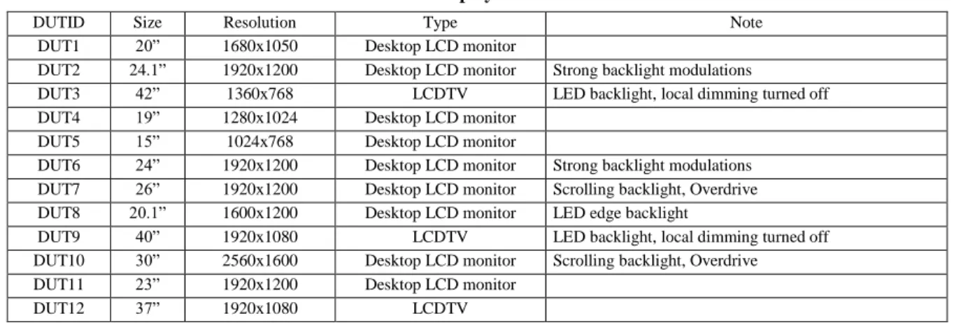
Displays that have been assessed in this work are described in Table 1. All of them are liquid-crystal displays (LCD). They were equipped with various features that are described in Table 1.

2.2 Temporal step response measurements

On each DUT, temporal step-responses of the pixels have been measured for 20 transitions from one gray level (𝑔𝑠𝑡𝑎𝑟𝑡) to another

(𝑔𝑒𝑛𝑑) among five. The following gray levels were used: 0, 63,

127, 191, and 255. Each of the 20 gray-to-gray transitions 𝑔𝑠𝑡𝑎𝑟𝑡 → 𝑔𝑒𝑛𝑑 have been measured 5 times on each DUT, except

for DUT3, DUT11 and DUT12 (only twice). Table 1: Displays under test.

DUTID Size Resolution Type Note DUT1 20” 1680x1050 Desktop LCD monitor

DUT2 24.1” 1920x1200 Desktop LCD monitor Strong backlight modulations

DUT3 42” 1360x768 LCDTV LED backlight, local dimming turned off DUT4 19” 1280x1024 Desktop LCD monitor

DUT5 15” 1024x768 Desktop LCD monitor

DUT6 24” 1920x1200 Desktop LCD monitor Strong backlight modulations DUT7 26” 1920x1200 Desktop LCD monitor Scrolling backlight, Overdrive DUT8 20.1” 1600x1200 Desktop LCD monitor LED edge backlight

DUT9 40” 1920x1080 LCDTV LED backlight, local dimming turned off DUT10 30” 2560x1600 Desktop LCD monitor Scrolling backlight, Overdrive

DUT11 23” 1920x1200 Desktop LCD monitor DUT12 37” 1920x1080 LCDTV

The light intensity emitted by the display was read by a photodiode positioned in close contact with the screen surface. The photodiode was surrounded by black velvet in order to reduce any scratches to the display surface and to shield any ambient light reaching the photodiode. The photodiode (Burr-Brown OPT101 monolithic photodiode with on chip transimpedance amplifier) has a fast response (28 µs from 10% to 90%, rise or fall time). The signal was read by an USB oscilloscope EasyScope II DS1M12 "Stingray" 2+1 Channel PC Digital Oscilloscope/Logger from USB instruments. The accuracy of the instrument has been tested with an LED light source connected to a function generator. Each transition has been measured sequentially by displaying each gray level during 20 frames, with a sampling period of 0.1 msec.

2.3 Moving edge temporal Profile

From these temporal step-responses, METP was then computed by convolving the waveform with a rectangular pulse of one frame time, in the same way as described in Tourancheau (2009)[5]. We then trimmed the METP from 15 frames before the transition to 15 frames after. This ensures that this 30-frame long waveform was clean of any residuals from the convolution or from the previous and next transitions.

3. Blur estimates

3.1 BET metric

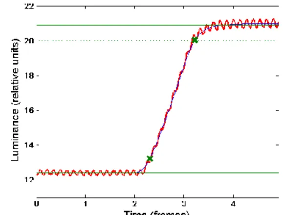
Blurred Edge Time (BET) is usually measured on the METP as the time interval from 10% to 90% of the METP luminance range. In order to determine 10% and 90% values of the METP, we need to estimate precisely the beginning relative luminance value 𝐵 and the ending relative luminance value 𝐸. This has been done by computing the average luminance value of samples corresponding to the first two frames and to the last two frames (respectively) of the METP.

Since some ripples can remain on METP after the convolution, it could have been necessary to apply some additional processing in order to determine for which samples it crossed the 10% and 90% values. This was done using a filtering with a Gaussian kernel with a standard deviation of 0.15 frames. An example of METP, with smoothed waveform is shown in Figure 1.

3.2 GET metric

The Gaussian Edge Time (GET) were measured according to Watson (2010)[8]. The following cumulative Gaussian function was fitted to the METP:

𝐺 𝑡 = 𝐵 + 𝐸 − 𝐵 1 𝜎 2𝜋 𝑡 −∞ exp − 𝑥 − 𝜇 2 2𝜎2 𝑑𝑥 𝐺 𝑡 = 𝐸 +𝐵 − 𝐸 2 erfc 𝑡 − 𝜇 𝜎 2

where 𝐸 and 𝐵 are beginning and ending relative luminance values, 𝑡 is the time in seconds, 𝜇 is the mean and 𝜎 is the standard deviation of the Gaussian, and erfc is the complementary error function. The parameter 𝜎 can be converted to an estimate of

BET that is referred to as the Gaussian Edge Time (GET) by:

𝐺𝐸𝑇 = 2.563𝜎

For additional accuracy, the fitting was done twice. First the parameters were estimated from the complete waveform. Then the

waveform was trimmed to the mean 𝜇 plus and minus a number 𝑁𝜎 of standard deviation𝑠 𝜎, and the fitting was repeated. Various

values of 𝑁𝜎 have been tested here, and the consistency between

BET and GET has been studied regarding this parameter. An

example of METP, with cumulative Gaussian function is shown in Figure 2.

3.3 Overdrive

Overdrive techniques to reduce liquid crystal cells response time can lead to overshoot or undershoot on the temporal step- responses, as well as on the METP. These artifacts are usually taken in account by measuring BET from -10% to 110% if these values are reached [9]. Since GET metric cannot reflect these particular distortions, we computed BET from 10% to 90% even in presence of overdrive, in order to compare both metrics equally.

Figure 1: Example of BET estimate for DUT10 and transition 191-255. Thick line (red) represents raw METP waveform, thin line (blue) is the smoothed METP waveform. Horizontal lines (green) figure the beginning and ending relative luminance values as well as the 10% and 90% levels. Samples from which BET is computed are marked with a cross.

Figure 2: Idem as Figure 1, GET estimate is obtained from the standard deviation of the cumulative Gaussian function obtained from the fitting (thin blue line).

14.1 / Sylvain Tourancheau

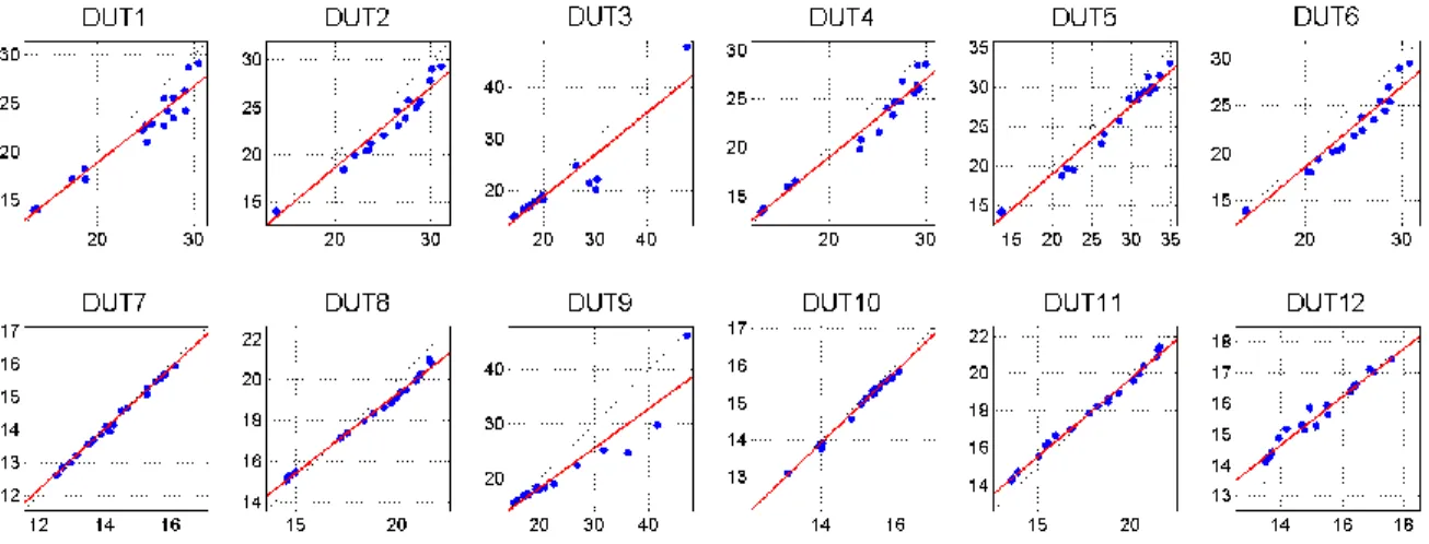
Figure 3: Scatter plot of GET as a function of BET for each DUT.

4. Results

4.1 Correspondence between BET and GET

We compared the correspondence between BET and GET according to the size of the METP waveform used during the second fitting to determine GET. As explained in Section 3.2, a second fitting was performed to increase the accuracy of the parameters. This second fitting was done on a trimmed METP waveform, from 𝜇 − 𝑁𝜎∙ 𝜎 to 𝜇 + 𝑁𝜎∙ 𝜎, with 𝜇 and 𝜎 the

parameters determined by the first fitting. The size of the METP waveform used for the second fitting was, therefore, 2𝑁𝜎∙ 𝜎.

Several values of 𝑁𝜎 were tested: 3, 4, 5, 7, and 10, and the linear

correlation coefficient between BET and GET were computed for each case. Results are presented in Figure 4. It can be observed that the linear correlation coefficient became better as the size of the waveform were increased. Note that when 𝑁𝜎 were higher

than 6, all correlation coefficients were higher than 0.96, except for DUT3 and DUT9 which are both LCDTVs with LED backlight.

As a conclusion, if we want GET to be a good predictor of BET, it is necessary to fit the cumulative Gaussian function on a METP waveform which is large enough. If not, some discrepancies can appear between both metrics due to a bad estimation of beginning and ending relative luminance values in the GET computation. In the following, we present a comparison between BET and GET with a value of 𝑁𝜎 fixed to 10.

Figure 4: Evolution of the linear correlation coefficient between BET and GET as a function of the size of the METP waveform used to determine GET.

In Figure 5 the correspondence between the two metrics BET and

GET is presented for each display. Table 2 presents the linear

correlation coefficient (LCC) and the root-mean-square error (RMSE) between BET and GET over all measurements and for each display. The linear relation 𝐺𝐸𝑇 = 𝑎𝐵𝐸𝑇 + 𝑏 is drawn by a red line in Figure 3 and the values of 𝑎 and 𝑏 are given in Table 2. On all DUT, the LCC between GET and BET is 0.969 and the corresponding linear relation is (cf. Figure 5):

𝐺𝐸𝑇 = 0.79 ∙ 𝐵𝐸𝑇 + 3.06

Table 2: Linear correlation and root-mean-square error between BET and GET for all DUT.

ID LCC a b RMSE DUT1 0.972 0.79 3.05 2.51 DUT2 0.978 0.85 1.61 2.34 DUT3 0.924 0.81 2.53 3.43 DUT4 0.984 0.81 2.73 2.12 DUT5 0.989 0.87 1.54 2.20 DUT6 0.977 0.85 1.53 2.41 DUT7 0.990 0.92 1.14 0.12 DUT8 0.996 0.78 3.68 0.70 DUT9 0.933 0.73 3.60 4.26 DUT10 0.984 0.96 0.48 0.16 DUT11 0.997 0.84 2.88 0.49 DUT12 0.982 0.78 3.73 0.55

4.2 Reproducibility of Measurements

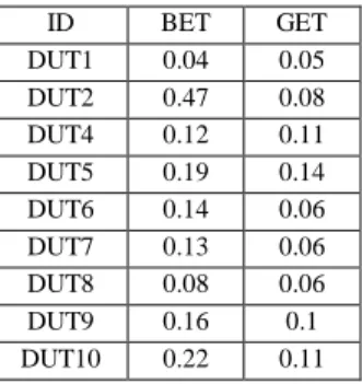
To evaluate the constancy and the reproducibility of measurements, we computed the standard deviation of the set of five measurements for each tested transition. The average of these standard deviation values over the 20 transitions is given for each display in Table 3, except for DUT3, DUT11 and DUT12 which have been measured only twice.

Globally, the average standard deviation between similar measurements is 0.17 for BET, and 0.09 for GET. We can observe from Table 3 that GET gives more stable results than BET. On DUT with strong backlight modulations such as DUT2 or DUT10, the METP waveform needs to be filtered to measure BET. This leads to high standard deviation values for 𝐵𝐸𝑇 since the position of backlight modulations regarding the frame refresh can be different from one measurement to another. In spite of this, GET estimates are particularly stable for these DUT.

Table 3: Average standard deviation of measurements for each DUT and for both metrics

ID BET GET DUT1 0.04 0.05 DUT2 0.47 0.08 DUT4 0.12 0.11 DUT5 0.19 0.14 DUT6 0.14 0.06 DUT7 0.13 0.06 DUT8 0.08 0.06 DUT9 0.16 0.1 DUT10 0.22 0.11

4.3 Comparison with user experience data

In this section we compared the metrics with the results of a user experience described previously [1]. In this subjective experiment users were asked to adjust the blur width of a simulated blurred edge until it matched the motion blur they perceived on a moving edge. From the responses of the observers a Mean Opinion BET (MOBET) were computed, as a subjective measure of the perceived blur in the used displays. This experiment has been led on 3 DUT: DUT10, DUT11 and DUT12.

If we observe these metrics’ correspondence to user experience, the fit is reasonable for such a simple metric with a correlation between BET and MOBET of 0.785 (RMSE = 2.05) and between

GET and MOBET of 0.780 (RMSE = 2.13). Not surprising

considering the close correspondence between the metrics, both

BET and GET have similar fits and it cannot be said that one is

better than the other based on this. It is also unclear whether a higher correlation is possible, given the variability among observers.

5. Conclusion

In this paper, we have investigated the relation between the metrics for motion blur BET and GET. Based on the measurements performed on 12 displays and 20 transitions each,

BET and GET are very similar with a 0.97 correlation. We have

shown that if we want GET to be a good predictor of BET it is

necessary to estimate it on a waveform with a large number of samples. However, there is no unique method of estimating 𝐵𝐸𝑇. For example, result will vary depending on the estimation of beginning and ending luminance values, and on the value of the filter standard deviation when filtering is necessary. From this point of view, 𝐺𝐸𝑇 metric is easier to standardize and permits to obtain similar results from one lab to another since there is no unknown parameters.

Despite the high correlation between BET and GET, relation between them is not identity. We have observed some discrepancies from one display to another but in a whole we obtained 𝐺𝐸𝑇 = 0.79 ∙ 𝐵𝐸𝑇 + 3.06.

Finally, both metrics provide a reasonable prediction of the mean opinion of observers, with a correlation is of 0.79. However, further research is required to build a metric able to predict user experience with accuracy.

6. Acknowledgements

This work was partly funded by VINNOVA (The Swedish Governmental Agency for Innovation Systems) which is hereby gratefully acknowledged. ABW was supported in part by NASA’s Space Human Factors Engineering Project, WBS 466199.

7. References

[1] Tourancheau, S., Le Callet, P., Brunnström, K., and Andrén, B., "Psychophysical study of LCD motion-blur perception", Proc.

of SPIE-IS&T Human Vision and Electronic Imaging XII, 7240,

B. Rogowitz and T. N. Pappas Eds., paper 51 (2009)

[2] Teunissen, K., Zhang, Y., Li, X., and Heynderickx, I., "Method for predicting motion artifacts in matrix displays",

Journal of the Society for Information Display 14, 957-964 (2006)

[3] Oka, K. and Enami, Y., "43.4: Moving Picture Response Time (MPRT) Measurement System", SID Symposium Digest of

Technical Papers 35(1), 1266-1269 (2004)

[4] Someya, J., "19.3: Correlation between Perceived Motion Blur and MPRT Measurement", SID Symposium Digest of Technical

Papers 36(1), 1018-1021 (2004)

[5] Tourancheau, S., Brunnström, K., Andrén, B., and Le Callet, P., "LCD motion-blur estimation using different measurement methods", Journal of the Society for Information Display 17, 239-249 (2009)

[6] Feng, X., Pan, H., and Daly, S., "Comparisons of motion-blur assessment strategies for newly emergent LCD and backlight driving technologies", Journal of the Society for Information

Display 16, 981-988 (2008)

[7] Watson, A. B., "31.1: Invited Paper: The Spatial Standard Observer: A Human Vision Model for Display Inspection", SID

Symposium Digest of Technical Papers 37(1), 1312-1315 (2006)

[8] Watson, A. B., "Display motion blur: Comparison of measurement methods." Journal of the Society for Information

Display 18(2): 179-190 (2010).

[9] VESA, "Flat Panel Display Measurements", Tech. Rep. Version 2.0, Video Electronics Standards Association, 2005.