Vibration Analysis of Euler-Bernoulli Beams Partially Immersed in a Viscous Fluid

(1)

HAL Id: hal-01366525

https://hal.archives-ouvertes.fr/hal-01366525

Submitted on 21 Dec 2017

HAL is a multi-disciplinary open access

archive for the deposit and dissemination of

sci-entific research documents, whether they are

pub-lished or not. The documents may come from

teaching and research institutions in France or

abroad, or from public or private research centers.

L’archive ouverte pluridisciplinaire HAL, est

destinée au dépôt et à la diffusion de documents

scientifiques de niveau recherche, publiés ou non,

émanant des établissements d’enseignement et de

recherche français ou étrangers, des laboratoires

publics ou privés.

Immersed in a Viscous Fluid

Wafik Abassi, Adil El Baroudi, Fulgence Razafimahéry

To cite this version:

Wafik Abassi, Adil El Baroudi, Fulgence Razafimahéry. Vibration Analysis of Euler-Bernoulli Beams

Partially Immersed in a Viscous Fluid. Physics Research International, 2016, 2016, pp.67613721

-6761372-14. �10.1155/2016/6761372�. �hal-01366525�

(2)

Research Article

Vibration Analysis of Euler-Bernoulli Beams Partially

Immersed in a Viscous Fluid

Wafik Abassi,

1

Adil El Baroudi,

1

and Fulgence Razafimahery

2 1_{Arts et M´etiers ParisTech, ENSAM Angers, 2 boulevard du Ronceray, 49035 Angers, France} 2_{IRMAR, Universit´e de Rennes 1, Campus de Beaulieu, 35042 Rennes Cedex, France}

Correspondence should be addressed to Adil El Baroudi; [email protected] Received 17 September 2015; Revised 20 January 2016; Accepted 27 January 2016 Academic Editor: Israel Felner

Copyright © 2016 Wafik Abassi et al. This is an open access article distributed under the Creative Commons Attribution License, which permits unrestricted use, distribution, and reproduction in any medium, provided the original work is properly cited. The vibrational characteristics of a microbeam are well known to strongly depend on the fluid in which the beam is immersed. In this paper, we present a detailed theoretical study of the modal analysis of microbeams partially immersed in a viscous fluid. A fixed-free microbeam vibrating in a viscous fluid is modeled using the Euler-Bernoulli equation for the beams. The unsteady Stokes equations are solved using a Helmholtz decomposition technique in a two-dimensional plane containing the microbeams cross sections. The symbolic software Mathematica is used in order to find the coupled vibration frequencies of beams with two portions. The frequency equation is deduced and analytically solved. The finite element method using Comsol Multiphysics software results is compared with present method for validation and an acceptable match between them was obtained. In the eigenanalysis, the frequency equation is generated by satisfying all boundary conditions. It is shown that the present formulation is an appropriate and new approach to tackle the problem with good accuracy.

1. Introduction

The objective of this paper is to provide an analytical method to calculate the coupled frequencies of vibration of microbeams partially immersed in a viscous fluid. The microbeams are clamped on one edge while the other edge is free.

The motivation of this work is to provide a theoretical model that can be used in the design and interpretation of density and viscosity sensors.

Due to their size and potential for highly sensitive and low cost compact device applications, microstructures are becoming increasingly attractive for sensing applications and have been studied extensively in recent years. Microstruc-tures are commonly used in atomic force microscopy (AFM) to probe surface properties and to measure interfacial forces [1–7], in biological and chemical sensors [8–10]. A precise modeling of the solid-fluid interaction and the determina-tion of the frequency response enable the measurement of the density and the rheological behavior of fluids [11–16]. Reference [16] uses finite element analysis (FEA) method in order to predict the dynamic response of the cantilever beam.

This method can be easily applied to the measurement of the fluid viscosity.

For microstructures, fluid viscosity can greatly affect their frequency response. Reference [7] presented a rigorous theoretical model for the frequency response of cantilever beams that are undergoing flexural vibrations and immersed in viscous fluids, which is of particular relevance to applica-tions of the AFM. The knowledge and understanding of the frequency analysis of microbeams are of fundamental practi-cal importance in application to the AFM.

The frequency analysis of a microbeam can be dramat-ically affected by the properties of the fluid in which it is immersed. Whereas calculation of the natural frequencies in vacuum can be performed routinely, analysis of the effects of immersion in fluid poses a formidable challenge. The modal response of an immersed microbeam can be considerably affected by the properties of fluid. The added mass effect due to the fluid structure interaction can, however, cause consid-erable variations in natural frequencies. The knowledge and understanding of this viscous fluid-structure coupling are lacking at present.

Volume 2016, Article ID 6761372, 14 pages http://dx.doi.org/10.1155/2016/6761372

(3)

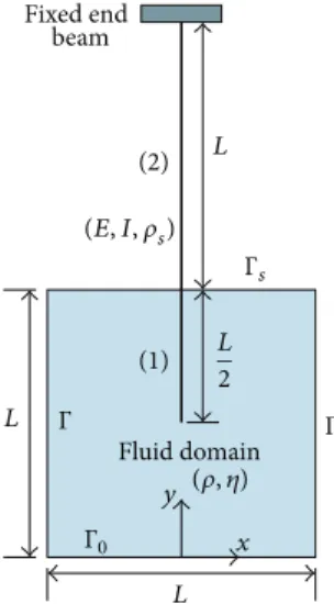
x y Fixed end beam Fluid domain (1) (2) L L L L 2 Γ Γ Γs Γ0 (𝜌, 𝜂) (E, I, 𝜌_s)

Figure 1: Sketch of beam composed of 2 uniform beam segments

(denoted by(1) and (2)) partially immersed in a fluid-filled

rectan-gular geometry.

In this contribution, we investigate the vibrational behav-ior of microbeams partially immersed in a viscous fluid, which describes the interrelation between the fluid’s density and viscosity. For a viscous fluid problem, the analytical formulation is based upon a convenient decomposition of the velocity field into two contributions, one being related to the scalar potential and the other being the vector potential. The solutions of the differential equations of motion turn out to be complex and can be conveniently treated with the aid of the symbolic software Mathematica. Furthermore, this work investigates the influence of the fluid’s viscosity on the vibrational behavior of the microbeams.

2. Modal Analysis of Beams and

Frequency Equation

Modal analysis of elastic immersed structures is needed in every modern construction and should have wide engineer-ing application. In this study, modal analysis is important to predict the dynamic behavior of the submerged beams. It is well known that the natural frequencies of the submerged elastic structures are different from those in vacuum. The effect of fluid forces on the immersed beam decreases the natural frequencies from those that would be measured in the vacuum. This decrease in the natural frequencies is caused by the increase of the kinetic energy of the fluid-beams system without a corresponding increase in strain energy. The Euler-Bernoulli beam is partially immersed inside rectangular fluid

domain (Figure 1). Consider a beam of length 3.06⋅10−2[m],

width 4.6⋅10−3_{[m], and thickness 1.27⋅10}−4_{[m] as shown in}

Figure 1, which corresponds to a model developed in [16]. The interaction between the fluid and the Euler-Bernoulli beams is taken into account to calculate the natural frequencies and mode shapes of the coupled system. The dynamics of each beam portion are treated separately. It is assumed that the beam has aligned neutral axis.

2.1. Mathematical Formulation. In this section we present the general theory for the dynamic deflection of beams partially submerged in a viscous fluid. A schematic depiction of beams partially submerged in viscous fluid is displayed in Figure 1. We begin by discussing some general assumptions and approximations taken into account in the present the-oretical model. It is assumed that the cross section of the beams is uniform over its entire length and the length of the beams greatly exceeds its width. Also the beams are an isotropic linearly elastic solid and internal frictional effects are negligible. The amplitude of the vibrations of the beams is small. In addition, we shall neglect all torsional effects in the beams and only consider the flexural modes of vibration and

we shall consider modes whose motion is strict in the

𝑥-direction. For beams vibrating at small amplitudes (small compared to the beams dimensions), the governing dynam-ical equations ignoring shear deformation and rotary inertia

effects for the transverse deflection𝑢_𝑖(𝑦, 𝑡) (𝑖 = 1 for

sub-merged portion and𝑖 = 2 for portion in vacuum) of uniform

elastic beams can be written in the form

EI𝜕 4_𝑢 1(𝑦, 𝑡) 𝜕𝑦4 + 𝜌𝑠𝑆𝜕 2_𝑢 1(𝑦, 𝑡) 𝜕𝑡2 = 𝑓fluid, 𝐿 2 ⩽ 𝑦 ⩽ 𝐿, (1) EI𝜕 4_𝑢 2(𝑦, 𝑡) 𝜕𝑦4 + 𝜌𝑠𝑆𝜕 2_𝑢 2(𝑦, 𝑡) 𝜕𝑡2 = 0, 𝐿 ⩽ 𝑦 ⩽ 2𝐿, (2)

where𝑢₁(𝑦, 𝑡) and 𝑢₂(𝑦, 𝑡) are the lateral deflections at

dis-tance𝑦 (spatial coordinate) along the length of the beams and

𝑡 is time; EI, 𝜌_𝑠, and𝑆 are the flexural rigidity, the mass per unit

volume, and the cross-sectional area of the beam, respectively. 𝑓fluidis the external force per unit length acting on the beam

in the direction of the flexural displacement, which is caused by the viscous fluid in the beams. The dynamics of each beam portion are treated separately.

For a beam moving in a viscous fluid, the applied load

𝑓_fluidcan be obtained by integrating the normal component

of the total force exerted by the fluid over the beam section.

To proceed with the analysis, the general form of𝑓_fluid is

required. We therefore examine the equations of motion for the fluid. For this, the viscous fluid mode shapes are first com-puted for the square domain fluid assuming the boundary conditions given in Figure 1. From conservations of mass and momentum, the motion of the fluid is governed by (see [17])

∇ ⋅ k = 0, (3)

𝜌𝜕k_𝜕𝑡 + 𝜌 (k ⋅ ∇) k = ∇ ⋅ 𝜎, (4)

in whichk = {V_𝑥, V_𝑦}𝑇is the fluid velocity vector,𝜌 is the

den-sity of the fluid, and𝜎 is the total fluid stress tensor (pressure

and viscous forces). Since the amplitude of vibration of each beam is small compared to its cross-sectional dimensions, it then follows that all nonlinear convective inertial effects in the fluid can be neglected, and the hydrodynamic loading on the beam will be a linear function of its displacement. This implies that the fluid dynamics can be modeled as

(4)

an unsteady linear Stokes flow. Assuming that the fluid is Newtonian, its constitutive equation is given by

𝜎 = 𝜏 − 𝑝I with 𝜏 = 𝜂 [∇k + (∇k)𝑇] , (5)

whereI is a unit tensor, 𝜂 is the dynamic viscosity, and 𝑝 is

the fluid pressure. The boundary conditions which define the fluid domain are

k ⋅ n = 0 on Γ, (6)

k = 0 on Γ₀, (7)

𝜎 ⋅ n = 0 on Γ𝑠. (8)

The equations of motion (3) and (4) are highly complex and coupled. However, a simpler set of equations can be

obtained by introducing scalar potentials𝜙 and 𝜓, known as

the Helmholtz decomposition [18] in a way which permits easily transferring the vector problem formulation ((3) and (4)) to scalar problem formulation. In flow fields, the velocity is thereby decomposed into a potential flow and a viscous

flow. In other words, the velocityv can be expressed as a sum

of the gradient of a scalar potential𝜙 and the curl of a vector

potentialΨ as follows [18]:

k = ∇𝜙 + ∇ × Ψ, (9)

whereΨ is a vector stream function. Using the problem

sym-metry, the vector potentialΨ reduces to a scalar equation; that

is,Ψ = (0, 0, 𝜓), using the condition ∇ ⋅ Ψ = 0, and

substitut-ing the above resolutions into (3) and (4), after some manipu-lations, the equation for the conservation of mass (3) becomes the Laplace equation

∇2_{𝜙 = 0} ₍₁₀₎

and the equation for the conservation of momentum (4) becomes ∇2_{𝜓 −}1 ] 𝜕𝜓 𝜕𝑡 = 0, 𝑝 + 𝜌𝜕𝜙_𝜕𝑡 = 0, (11)

where] is the kinematic fluid viscosity and ∇2 = 𝜕2/𝜕𝑥2+

𝜕2_/𝜕𝑦2_{is the Laplacian operator. Thus, the Stokes equation is}

reduced to formulation (10) and (11). Moreover, adopting the

Cartesian coordinate system(𝑥, 𝑦) and using expression (9),

the velocity components,V = (V_𝑥, V_𝑦), may be expressed as

simple functions of compressional and shear wave potentials in the form V_𝑥= 𝜕𝜙 𝜕𝑥+ 𝜕𝜓 𝜕𝑦, V_𝑦= 𝜕𝜙 𝜕𝑦 − 𝜕𝜓 𝜕𝑥 (12)

and the pertinent stress-velocity relations are

𝜎𝑥𝑥= 𝜌𝜕𝜙_𝜕𝑡 + 2𝜂𝜕V_𝜕𝑥𝑥, 𝜎_𝑥𝑦 = 𝜂 (𝜕V𝑥 𝜕𝑦 + 𝜕V_𝑦 𝜕𝑥) , 𝜎_𝑦𝑦= 𝜌𝜕𝜙 𝜕𝑡 + 2𝜂 𝜕V_𝑦 𝜕𝑦. (13)

2.1.1. Field Expansions. Consider time harmonic motion

throughout with angular frequency𝜔 and with the exp(𝑖𝜔𝑡)

dependence suppressed for simplicity. Applying the classical technique of separation of variables in the Cartesian coordi-nates, the solution of (10) and (11) after some manipulations, and taking into account boundary condition (6) can be shown to be

𝜓 = sin (𝛽𝑥) [𝐴 cos (𝛿𝑦) + 𝐵 sin (𝛿𝑦)] , (14)

𝜙 = cos (𝛽𝑥) [𝐶 cos (𝜆𝑦) + 𝐷 sin (𝜆𝑦)] , (15)

𝑝 = 𝜂𝛼2cos(𝛽𝑥) [𝐶 cos (𝜆𝑦) + 𝐷 sin (𝜆𝑦)] (16)

with the complex-valued coefficients 𝜆 = 𝑗𝛽,

𝛿 = 𝑗√𝛽2_{− 𝛼}2_,

𝛼 = 1 − 𝑗

√2 √ 𝜔],

(17)

where 𝛽 = 𝑛𝜋/𝐿 and 𝑛 is an integer. 𝐴, 𝐵, 𝐶, and 𝐷

are unknown coefficients which will be determined later by imposing the appropriate boundary conditions. Hence, the fluid particle velocity field can be determined from (12) in the form

V_𝑥= sin (𝛽𝑥) {𝛿[𝐵 cos (𝛿𝑦) − 𝐴 sin (𝛿𝑦)]

− 𝛽 [𝐶 cos (𝜆𝑦) + 𝐷 sin (𝜆𝑦)]} , (18)

V_𝑦= cos (𝛽𝑥) {𝜆 [𝐷 cos (𝜆𝑦) − 𝐶 sin (𝜆𝑦)]

− 𝛽 [𝐴 cos (𝛿𝑦) + 𝐵 sin (𝛿𝑦)]} . (19)

Consequently, direct substitution of the expansions (14)–(19) into the stress-velocity relations (13), after some manipula-tions, leads to

𝜎𝑥𝑥= 𝜂 cos (𝛽𝑥) {2𝛽𝛿[𝐵 cos (𝛿𝑦) − 𝐴 sin (𝛿𝑦)]

(5)

𝜎𝑦𝑦= 𝜂 cos (𝛽𝑥) {2𝛽𝛿[𝐴 sin (𝛿𝑦) − 𝐵 cos (𝛿𝑦)] − (2𝜆2+ 𝛼2) [𝐶 cos (𝜆𝑦) + 𝐷 sin (𝜆𝑦)]} , (21) 𝜎_𝑥𝑦= 𝜂 sin (𝛽𝑥) ⋅ {(2𝛽2− 𝛼2) [𝐴 cos (𝛿𝑦) + 𝐵 sin (𝛿𝑦)] + 2𝛽𝜆 [𝐶 sin (𝜆𝑦) − 𝐷 cos (𝜆𝑦)]} . (22)

In order to determine the unknown constants, the appropri-ate boundary conditions (7) and (8) must be explicitly used. Substituting the total fluid stress tensor components (20)– (22) into boundary conditions equations (8) and velocity components (18)-(19) into boundary conditions equations (7), and after some considerable algebraic manipulation, the

scalar potentials𝜙 and 𝜓 become

𝜓 = 𝐴 sin (𝛽𝑥) [cos (𝛿𝑦) +𝛽_𝛿2Φ sin (𝛿𝑦)] , (23)

𝜙 = 𝐴 cos (𝛽𝑥) [𝛽Φ cos (𝜆𝑦) +𝛽 𝜆sin(𝜆𝑦)] , (24) where Φ = 2𝛿 sin (𝛿𝐿) + (2𝛽 2_{− 𝛼}2_{) (sin (𝜆𝐿) /𝜆)} 2𝛽2_cos_{(𝛿𝐿) − (2𝛽}2_{− 𝛼}2_{) cos (𝜆𝐿)} . (25)

Using the expressions of𝜓 and 𝜙 from (23) and (24), in (12),

we have the following expressions for the velocity compo-nents: V𝑥= 𝐴 sin (𝛽𝑥) {𝛿[𝛽 2 𝛿Φ cos (𝛿𝑦) − sin (𝛿𝑦)] − 𝛽 [𝛽Φ cos (𝜆𝑦) +𝛽_𝜆sin(𝜆𝑦)]} , (26) V_𝑦= 𝐴 cos (𝛽𝑥) {𝜆 [𝛽 𝜆cos(𝜆𝑦) − 𝛽Φ sin (𝜆𝑦)] − 𝛽 [cos (𝛿𝑦) + 𝛽2 𝛿Φ sin (𝛿𝑦)]} . (27)

Components of the stress tensor can be obtained by

substitut-ing the expressions of velocity componentsV_𝑥;V_𝑦, from (26)

and (27), and the expression of scalar potential𝜙 from (24) in

(13) which comes out as

𝜎_𝑥𝑥= 𝐴𝜂 cos (𝛽𝑥) {2𝛽𝛿[𝛽2

𝛿Φ cos (𝛿𝑦) − sin (𝛿𝑦)]

− (2𝛽2+ 𝛼2) [𝛽Φ cos (𝜆𝑦) +𝛽

𝜆sin(𝜆𝑦)]} ,

(28)

𝜎_𝑦𝑦= 𝐴𝜂 cos (𝛽𝑥) {2𝛽𝛿[sin (𝛿𝑦) −𝛽_𝛿2Φ cos (𝛿𝑦)]

− (2𝜆2+ 𝛼2) [𝛽Φ cos (𝜆𝑦) +𝛽 𝜆sin(𝜆𝑦)]} , (29) 𝜎_𝑥𝑦= 𝐴𝜂 sin (𝛽𝑥) ⋅ {(2𝛽2− 𝛼2) [cos (𝛿𝑦) + 𝛽2 𝛿Φ sin (𝛿𝑦)] + 2𝛽𝜆 [𝛽Φ sin (𝜆𝑦) −𝛽 𝜆cos(𝜆𝑦)]} . (30)

Now we can integrate the normal component of the total force exerted by the fluid over the beam section in order to obtain the external force per unit length acting on the beam

in the direction of the flexural displacement𝑓_fluid. Hence, the

deflection of the immersed part of the beam (which is equal

to𝑢₁(𝑦, 𝑡) = 𝑢₁(𝑦) exp (𝑗𝜔𝑡)) can be determined from (1) and

(28) in the form 𝑢󸀠󸀠󸀠󸀠₁ (𝑦) − 𝜌𝑠𝑆𝜔2 EI 𝑢1(𝑦) =2𝐴𝛽𝜂 cos (𝛽𝐿/2) EI {𝛽 2_{Φ cos (𝛿𝑦) − 𝛿 sin (𝛿𝑦)} − (𝛽2+𝛼2 2 ) [Φ cos (𝜆𝑦) + sin(𝜆𝑦) 𝜆 ]} , (31)

where primes denote differentiation with respect to the

posi-tion variable𝑦.

2.2. Method of Solution and Frequency Equation. The general solutions of the ordinary differential equations (31) and (2) for the beams system, as shown in Figure 1, can be written in dif-ferent segments in terms of trigonometric functions and rep-resent propagating waves and hyperbolic functions reprep-resent evanescent waves as

𝑢₁(𝑦) = 𝐴₁cos(Ω𝑦) + 𝐵₁sin(Ω𝑦) + 𝐶₁cosh(Ω𝑦)

+ 𝐷₁sinh(Ω𝑦) +2𝐴𝛽𝜂 cos (𝛽𝐿/2) EI { 𝛿 sin (𝛿𝑦) − 𝛽2_{Φ cos (𝛿𝑦)} Ω4_{− 𝛿}4 +𝛽2+ 𝛼2/2 Ω4_{− 𝜆}4 [Φ cos (𝜆𝑦) + sin(𝜆𝑦) 𝜆 ]} , (32)

𝑢₂(𝑦) = 𝐴₂cos(Ω𝑦) + 𝐵₂sin(Ω𝑦) + 𝐶₂cosh(Ω𝑦)

+ 𝐷₂sinh(Ω𝑦) , (33)

whereΩ is the flexural wavenumber and is given by

Ω = √𝜔 (𝜌𝑠𝑆

EI)

1/4

(6)

Equation (32) shows that the parameters 𝜔_𝑐= (𝑛𝜋 𝐿 ) 2 √ EI 𝜌_𝑠𝑆, 𝜔_𝑐= (𝑛𝜋/𝐿)2 √𝜌𝑠𝑆/EI + 1/] (35)

are resonance frequency parameters and can be plotted for

different values of𝑛.

The nine constants𝐴₁,𝐵₁,𝐶₁,𝐷₁,𝐴₂,𝐵₂,𝐶₂,𝐷₂, and𝐴

can be found by imposing the following boundary conditions. Equations (32) and (33) are the general solution for the vibra-tion modes of beams partially immersed in fluid. In the case of a coupled system, the effect of fluid viscosity on the flexible beams must be considered. On the fluid-beams interface, the normal velocity must be continuous. Therefore, the fluid

velocity and the deflection of a beam𝑢₁satisfy the relation

V_𝑥󵄨󵄨󵄨󵄨_𝑥=𝐿/2= 𝑗𝜔𝑢₁(𝑦) , 𝐿

2 ⩽ 𝑦 ⩽ 𝐿. (36)

Substituting (26) and (32) into (36), and after some manipu-lations, leads to the following equation:

𝐴 [1 + 2𝜆𝜔𝜂 EI(Ω4− 𝛿4) tan (𝛽𝐿/2)] ⋅ [𝛽2Φ cos (𝛿𝑦) − 𝛿 sin (𝛿𝑦)] − 𝐴 [𝛽2+ 2𝜆𝜔𝜂 (𝛽 2_{+ 𝛼}2_/2) EI(Ω4− 𝜆4) tan (𝛽𝐿/2)] ⋅ [Φ cos (𝜆𝑦) + sin(𝜆𝑦) 𝜆 ] = 𝑗𝜔

sin(𝛽𝐿/2)[𝐴1cos(Ω𝑦) + 𝐵1sin(Ω𝑦)]

+ 𝑗𝜔

sin(𝛽𝐿/2)[𝐶1cosh(Ω𝑦) + 𝐷1sinh(Ω𝑦)] .

(37)

Both sides of (37) are integrated over𝐿/2 < 𝑦 < 𝐿 to yield the

following equation:

𝐴 = 𝑗𝜔

Υ sin (𝛽𝐿/2)(𝐴1𝐼1+ 𝐵1𝐼2+ 𝐶1𝐼3+ 𝐷1𝐼4) , (38)

whereΥ and the coefficients 𝐼₁,𝐼₂,𝐼₃, and𝐼₄are written down

explicitly in Appendix E. Now the expression of the lateral movement of the submerged beams in contact with the fluid

𝑢₁can be formulated using (32) and taking into account (38)

as 𝑢₁(𝑦) = 𝐴₁[cos (Ω𝑦) + 𝐼₁𝑈 (𝑦)] + 𝐵₁[sin (Ω𝑦) + 𝐼₂𝑈 (𝑦)] + 𝐶₁[cosh (Ω𝑦) + 𝐼₃𝑈 (𝑦)] + 𝐷₁[sinh (Ω𝑦) + 𝐼₄𝑈 (𝑦)] , (39) where 𝑈 (𝑦) = 2𝜆𝜂𝜔 EIΥ tan (𝛽𝐿/2)[ 𝛿 sin (𝛿𝑦) − 𝛽2_{Φ cos (𝛿𝑦)} Ω4_{− 𝛿}4 +𝛽2+ 𝛼2/2 Ω4_{− 𝜆}4 (Φ cos (𝜆𝑦) + sin(𝜆𝑦) 𝜆 )] . (40)

Now, to derive the frequency equation of beams partially immersed in fluid, one assumes that, on the interface between

each portion of the beam at the position𝑦 = 𝐿, the deflection,

the rotation angle, the internal shear force, and bending moment of the beam must be continuous. This is satisfied when 𝑢₁(𝐿) = 𝑢₂(𝐿) , 𝑢󸀠 1(𝐿) = 𝑢󸀠2(𝐿) , 𝑢󸀠󸀠₁ (𝐿) = 𝑢󸀠󸀠₂(𝐿) , 𝑢󸀠󸀠󸀠₁ (𝐿) = 𝑢󸀠󸀠󸀠₂ (𝐿) . (41)

To complete the formulation of the boundary-value problem, the four boundary conditions for the beam ends (𝑦 = 𝐿/2 = 𝑎

and𝑦 = 2𝐿 = 𝑏) considered in this work are specified as

follows: 𝑢󸀠󸀠₁(𝑎) = 0, 𝑢󸀠󸀠󸀠₁ (𝑎) = 0, 𝑢₂(𝑏) = 0, 𝑢₂󸀠(𝑏) = 0. (42)

Combining the boundary conditions ((41) and (42)) with (33) and (39) yields the following linear homogeneous system of eight equations:

MX = 0, X = [𝐴₁, 𝐵₁, 𝐶₁, 𝐷₁, 𝐴₂, 𝐵₂, 𝐶₂, 𝐷₂]𝑇, (43)

where M is a 8 × 8 matrix whose elements are designated

as𝑀_𝑖𝑗. This system can have nontrivial solutions only if the

determinant of the matrix M is zero, leading to the

fre-quency equation. The matrixM is written down explicitly in

Appendix F.

3. Analytical and Numerical

Results and Validation

The model that was developed in Section 2 can be validated by comparing the analytical results to model results calculated using Comsol Multiphysics FEM Simulation Software. This

comparison used beams with Young’s modulus being 𝐸 =

200⋅109_{[Pa], Poisson’s ratio being}_{] = 0.3, and density being}

𝜌 = 9450 [kg/m3]. The fluid used in the rectangular container

for which density of965 [kg⋅m−3] and dynamic’s viscosity of

0.1 [Pa⋅s] is assumed.

For coupled vibration analysis of beams partially immersed in a viscous fluid, the accuracy of the present method has been compared with the results obtained with

(7)

Table 1: The first 24 coupled natural angular frequencies 𝜔 of the partially immersed beams in a viscous fluid. Comparison of frequency between FEM and present method.

Order Present FEM Difference(%)

1 4.90 4.86 0.82 2 18.18 17.91 1.50 3 20.26 20.01 1.24 4 21.11 20.86 1.19 5 24.68 24.50 0.73 6 30.48 30.20 0.92 7 31.59 31.44 0.47 8 39.24 38.91 0.84 9 44.68 44.51 0.38 10 47.65 47.31 0.71 11 50.20 49.72 0.96 12 54.68 54.02 1.22 13 56.10 55.33 1.39 14 61.47 61.25 0.35 15 61.90 61.36 0.88 16 64.57 64.15 0.65 17 67.29 66.72 0.85 18 73.47 72.99 0.65 19 79.63 79.21 0.53 20 80.06 79.42 0.80 21 85.67 85.41 0.30 22 87.58 87.09 0.56 23 91.33 90.85 0.52 24 97.44 97.10 0.35

Comsol Multiphysics FEM Simulation Software. The FEM

used model had585039 number of degrees of freedom and

was analyzed using the algorithm based on the UMFPACK method [19].

In this paper the comparison of the values of the angular

frequency parameter𝜔 is given in Table 1. As one can see from

the comparison, very good agreement with those of FEM is obtained.

With the derived eigenfrequency equations, natural

fre-quencies𝜔 are calculated in the software Mathematica. To

validate the analytical results, the natural frequencies and mode shapes are also computed using Comsol Multiphysics FEM Simulation Software. The natural frequencies are com-puted directly from determinant of (43).

Table 1 shows the comparison of the first 24 natural fre-quencies and the corresponding mode shapes of viscous fluid by FEM and the present method (43). The good agreement is observed between the results of the present method and

those of FEM and the relative difference(100 × (Present −

FEM)/FEM) is ⩽2%. This shows that the algorithm imple-mented in Comsol Multiphysics [20] software for numerical computation is highly reliable and accurate. Mesh refinement can significantly decrease the relative difference.

The two possible first coupled mode shapes are repre-sented in Figure 2. A very good agreement with Figure 3 of [16] confirms the adequate implementation of the method in the FEM software.

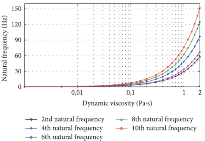
Figures 3 and 4 show the influence of fluid’s viscosity on the odd and even natural frequencies. It is seen that

Figure 2: Two possible first coupled mode shapes.

0,01 0,1 1 2 0 30 60 90 120 150 N at ural f req uenc y (H z) 1st natural frequency 3rd natural frequency 5th natural frequency 7th natural frequency 9th natural frequency Dynamic viscosity (Pa·s)

Figure 3: The influence of fluid’s viscosity on the first five odd natural frequencies. 0,01 0,1 1 2 0 30 60 90 120 150 N at ural f req uenc y (H z) 2nd natural frequency 4th natural frequency 6th natural frequency 8th natural frequency 10th natural frequency Dynamic viscosity (Pa·s)

Figure 4: The influence of fluid’s viscosity on the first five even natural frequencies.

(8)

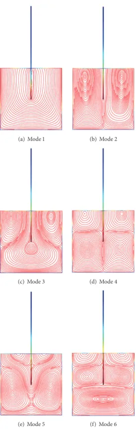
(a) Mode 1 (b) Mode 2

(c) Mode 3 (d) Mode 4

(e) Mode 5 (f) Mode 6

Figure 5: View of displacement filled of beams and Stokes eddies, showing various mode shapes for the coupled vibration.

the effect of viscosity is very interesting and decreases the frequency of beams. These figures show also for small fluid’s viscosity that the model is not suitable to describe properly the vibrational behavior of beams immersed in a viscous fluid. In this case, the most appropriate model is the

model developed in [21]. In other words, the viscosity terms can be neglected and the resulting model is called inertial coupling [22].

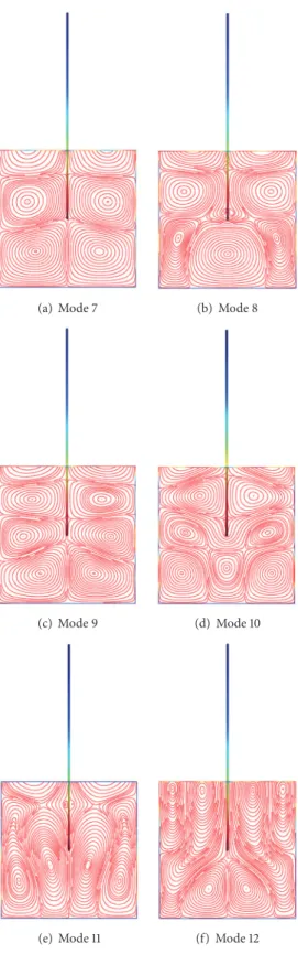
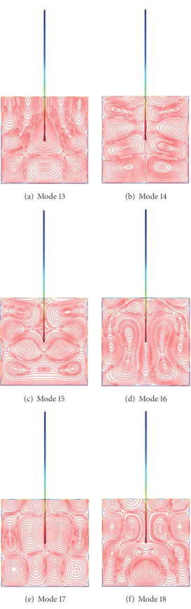
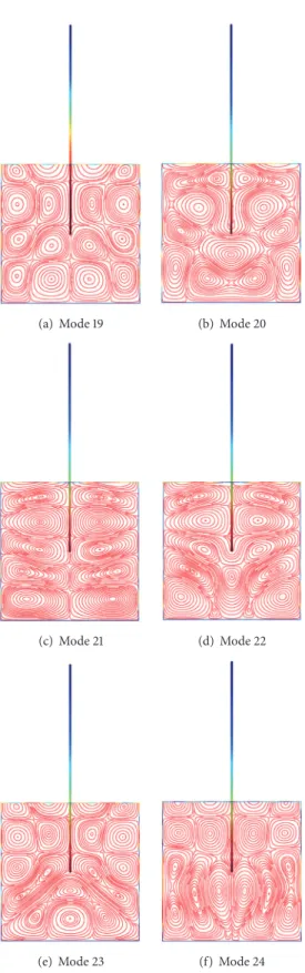
Figures 5(a)–5(f)–8(a)–8(f) obtained by Comsol show the first 24 coupled modal shapes with the corresponding

(9)

eigenvalues𝜔. In these figures, solid lines denote streamlines

(i.e., Stokes eddies) caused by system boundaries and fluid structure interaction. In addition, the formation of Stokes eddies is not affected by the presence of an obstacle (beam)

in the fluid domain. As expected these Stokes eddies increase when the angular frequency is raised like in the case without obstacle. Finally, these Stokes eddies are symmetric with respect to the obstacle.

(10)

4. Conclusion

This paper has presented an analytical method to understand the modal behavior of beams partially immersed in a viscous fluid. The validity of the present solution is solidly confirmed

numerically. The main application of the proposed method is in characterization of rheological properties of viscous mate-rials [16]. In addition the study can be also extended further for the optimization tool for complex engineering design problems.

(11)

(12)

Appendices

A. Analytical Expression for

the Scalar Potentials

(i) Solution of (11). A time harmonic dependence exp(𝑗𝜔𝑡) is

assumed, with𝑗 being the imaginary unit, 𝜔 being the circular

frequency, and𝑡 being the time. We introduce a new auxiliary

variable𝛼 defined as 𝛼 = ((1 − 𝑗)/√2)√𝜔/]. The first of the

two subequations (Equation (11)) consists of determining the

scalar potential𝜓(𝑥, 𝑦) satisfying the homogeneous diffusion

equation

𝜕2_𝜓

𝜕𝑥2 +

𝜕2_𝜓

𝜕𝑦2 + 𝛼2𝜓 = 0. (A.1)

By separation of variables, the scalar potential𝜓(𝑥, 𝑦) can be

written as

𝜓 (𝑥, 𝑦) = 𝜓𝑥(𝑥) 𝜓𝑦(𝑦) , (A.2)

where𝜓_𝑥(𝑥) and 𝜓_𝑦(𝑦) are given by the following ordinary

differential equation: 1 𝜓_𝑥(𝑥) 𝑑2_𝜓 𝑥(𝑥) 𝑑𝑥2 +_𝜓 1 𝑦(𝑦) 𝑑2𝜓𝑦(𝑦) 𝑑𝑦2 + 𝛼2= 0. (A.3)

The linear independent solutions of these equation yield a general pressure field of the form

𝜓 (𝑥, 𝑦) = [𝑎₁cos(𝛽𝑥) + 𝑎₂sin(𝛽𝑥)]

⋅ [𝑎₃cos(𝛿𝑦) + 𝑎₄sin(𝛿𝑦)] , (A.4)

where𝑎₁,𝑎₂,𝑎₃, and𝑎₄are unknown coefficients which will

be determined later by imposing the appropriate boundary conditions.

(ii) Solution of (10). In a similar manner, the solution of (10) can be defined. The solution consists of determining the

scalar potential𝜙(𝑥, 𝑦) satisfying the Laplace equation

𝜕2_𝜙

𝜕𝑥2 +

𝜕2_𝜙

𝜕𝑦2 = 0. (A.5)

By separation of variables, after some elementary manipula-tions, the linear solution of these equations yields a general

scalar potential𝜙(𝑥, 𝑦) of the form

𝜙 (𝑥, 𝑦) = [𝑎₁sin(𝛽𝑥) − 𝑎₂cos(𝛽𝑥)]

⋅ [𝑎₅cos(𝜆𝑦) + 𝑎₆sin(𝜆𝑦)] . (A.6)

(iii) Boundary Conditions. The boundary condition equation (6) can be expressed by 𝜕𝜙 𝜕𝑥󵄨󵄨󵄨󵄨󵄨󵄨󵄨󵄨𝑥=0+ 𝜕𝜓 𝜕𝑦󵄨󵄨󵄨󵄨󵄨󵄨󵄨󵄨_𝑥=0 = 0, 𝜕𝜙 𝜕𝑥󵄨󵄨󵄨󵄨󵄨󵄨󵄨󵄨𝑥=𝐿+ 𝜕𝜓 𝜕𝑦󵄨󵄨󵄨󵄨󵄨󵄨󵄨󵄨_𝑥=𝐿= 0. (A.7)

Substituting 𝜙(𝑥, 𝑦) and 𝜓(𝑥, 𝑦) into boundary condition

above gives the analytical solution for potential function (14) and (15). Now using the second equation of (11), the pressure can be presented by (16).

B. No-Slip Condition and Stress-Free

Boundary Condition

In this paper the interfaceΓ₀(7) is assumed to be rigid, leading

to

V_𝑥󵄨󵄨󵄨󵄨_𝑦=0= 0,

V𝑦󵄨󵄨󵄨󵄨_󵄨_𝑦=0= 0.

(B.1)

Substituting (18) and (19) into above rigid boundary equa-tions gives

𝛿 𝐵 − 𝛽𝐶 = 0,

𝜆𝐷 − 𝛽𝐴 = 0. (B.2)

The interfaceΓ_𝑠 (8) is assumed to be free boundary stress,

leading to

𝜎_𝑥𝑦󵄨󵄨󵄨󵄨_󵄨_𝑦=𝐿= 0,

𝜎_𝑦𝑦󵄨󵄨󵄨󵄨_󵄨_𝑦=𝐿= 0. (B.3)

Substituting (21) and (22) into above free boundary stress equations gives the first conditions, for example,

𝐴𝛽2𝛿 sin (𝛿𝐿) + (2𝛽

2_{− 𝛼}2_{) (sin (𝜆𝐿) /𝜆)}

2𝛽2_cos_{(𝛿𝐿) − (2𝛽}2_{− 𝛼}2_{) cos (𝜆𝐿)} − 𝐶 = 0. (B.4)

Note that, from the above equation, we can obtain

𝐶 = 𝐴𝛽2𝛿 sin (𝛿𝐿) + (2𝛽

2_{− 𝛼}2_{) (sin (𝜆𝐿) /𝜆)}

2𝛽2_cos_{(𝛿𝐿) − (2𝛽}2_{− 𝛼}2_{) cos (𝜆𝐿)}

= 𝐴𝛽Φ.

(B.5)

By replacing the constants into (14) and (15), the potential

functions𝜙 and 𝜓 can be expressed by

𝜓 = sin (𝛽𝑥) [𝐴 cos (𝛿𝑦) + 𝐵 sin (𝛿𝑦)]

= sin (𝛽𝑥) [𝐴 cos (𝛿𝑦) +𝛽

𝛿𝐶 sin (𝛿𝑦)]

= sin (𝛽𝑥) [𝐴 cos (𝛿𝑦) +𝛽_𝛿𝐴𝛽Φ sin (𝛿𝑦)]

= 𝐴 sin (𝛽𝑥) [cos (𝛿𝑦) +𝛽_𝛿2Φ sin (𝛿𝑦)] ,

(B.6)

𝜙 = cos (𝛽𝑥) [𝐶 cos (𝜆𝑦) + 𝐷 sin (𝜆𝑦)]

= cos (𝛽𝑥) [𝐴𝛽Φ cos (𝜆𝑦) +𝛽

𝜆𝐴 sin (𝜆𝑦)]

= 𝐴 cos (𝛽𝑥) [𝛽Φ cos (𝜆𝑦) +𝛽

𝜆sin(𝜆𝑦)] .

(13)

C. Solution of the Submerged Part of the Beam

We postulate the following solution of (1):

EI𝜕 4_𝑢 1(𝑦, 𝑡) 𝜕𝑦4 + 𝜌𝑠𝑆𝜕 2_𝑢 1(𝑦, 𝑡) 𝜕𝑡2 = 𝜎𝑥𝑥(𝐿₂, 𝑦) (C.1)

describing the lateral deflexion of the submerged beam

𝑢₁= 𝑢₁(𝑦) exp (𝑗𝜔𝑡) . (C.2)

Substitution into (1) and taking into account (28) yield

EI𝑑 4_𝑢 1(𝑦) 𝑑𝑦4 − 𝜌𝑠𝑆𝜔2𝑢1(𝑦) = 𝐴𝜂 cos (𝛽𝐿₂ ) ⋅ {2𝛽𝛿[𝛽2 𝛿Φ cos (𝛿𝑦) − sin (𝛿𝑦)] − (2𝛽2+ 𝛼2) [𝛽Φ cos (𝜆𝑦) +𝛽_𝜆sin(𝜆𝑦)]} . (C.3)

The software Mathematica was used in order to obtain (32) solution of the above equation. Similarly, we can also find (33) solution of (2) describing the lateral deflexion of the beam in vacuum.

D. Frequency Equation

For nontrivial solution, the determinant of the matricesM

must be equal to zero

detM = 0. (DM)

This equation indicates a relationship between the kinematic

fluid viscosity], fluid density 𝜌, angular frequency 𝜔, and the

elastic constants. For given material and geometric proper-ties, (DM) constitutes an implicit transcendental function of 𝑛 and 𝜔. The roots 𝜔 may be computed for a fixed 𝑛.

E. Auxiliary Coefficients

The coefficients Υ, 𝐼₁, 𝐼₂, 𝐼₃, and𝐼₄ in (38) are defined as

follows: Υ = ∫𝐿 𝑎 {[1 + Λ Ω4_{− 𝛿}4] [𝛽2Φ cos (𝛿𝑦) − 𝛿 sin (𝛿𝑦)] − [Λ (𝛽 2_{+ 𝛼}2_/2) Ω4_{− 𝜆}4 + 𝛽2] ⋅ [Φ cos (𝜆𝑦) +sin(𝜆𝑦) 𝜆 ]} 𝑑𝑦, (E.1) where Λ = 2𝜆𝜔𝜂 EI tan(𝛽𝐿/2), 𝐼1= ∫ 𝐿 𝑎 cos(Ω𝑦) 𝑑𝑦, 𝐼₂= ∫𝐿 𝑎 sin(Ω𝑦) 𝑑𝑦, 𝐼₃= ∫𝐿 𝑎 cosh(Ω𝑦) 𝑑𝑦, 𝐼₄= ∫𝐿 𝑎 sinh(Ω𝑦) 𝑑𝑦. (E.2)

F. The Elements of the

M Matrix

The matrixM in (13) is defined as follows:

M = [M₁₁, M₂₁, M₃₁, M₄₁, M₅₁, M₆₁, M₇₁, M₈₁]𝑇, (F.1) where M₁₁= {𝑀₁₁, 𝑀₁₂, 𝑀₁₃, 𝑀₁₄, 𝑀₁₅, 𝑀₁₆, 𝑀₁₇, 𝑀₁₈} , M₂₁= {𝑀₂₁, 𝑀₂₂, 𝑀₂₃, 𝑀₂₄, 𝑀₂₅, 𝑀₂₆, 𝑀₂₇, 𝑀₂₈} , M₃₁= {𝑀₃₁, 𝑀₃₂, 𝑀₃₃, 𝑀₃₄, 𝑀₃₅, 𝑀₃₆, 𝑀₃₇, 𝑀₃₈} , M₄₁= {𝑀₄₁, 𝑀₄₂, 𝑀₄₃, 𝑀₄₄, 𝑀₄₅, 𝑀₄₆, 𝑀₄₇, 𝑀₄₈} , M₅₁= {𝑀₅₁, 𝑀₅₂, 𝑀₅₃, 𝑀₅₄, 0, 0, 0, 0} , M₆₁= {𝑀₆₁, 𝑀₆₂, 𝑀₆₃, 𝑀₆₄, 0, 0, 0, 0} , M₇₁= {0, 0, 0, 0, 𝑀₇₅, 𝑀₇₆, 𝑀₇₇, 𝑀₇₈} , M₈₁= {0, 0, 0, 0, 𝑀₈₅, 𝑀₈₆, 𝑀₈₇, 𝑀₈₈} , (F.2) where 𝑀11= 𝑔1(𝐿) , 𝑀12= 𝑔2(𝐿) , 𝑀13= 𝑔3(𝐿) , 𝑀14= 𝑔4(𝐿) , 𝑀15= 𝑓1(𝐿) , 𝑀16= 𝑓2(𝐿) , 𝑀17= 𝑓3(𝐿) , 𝑀18= 𝑓4(𝐿) , 𝑀₂₁= 𝑔₁󸀠(𝐿) , 𝑀₂₂= 𝑔₂󸀠(𝐿) , 𝑀₂₃= 𝑔₃󸀠(𝐿) , 𝑀₂₄= 𝑔₄󸀠(𝐿) ,

(14)

𝑀₂₅= 𝑓₁󸀠(𝐿) , 𝑀₂₆= 𝑓₂󸀠(𝐿) , 𝑀₂₇= 𝑓₃󸀠(𝐿) , 𝑀28= 𝑓4󸀠(𝐿) , 𝑀₃₁= 𝑔₁󸀠󸀠(𝐿) , 𝑀₃₂= 𝑔₂󸀠󸀠(𝐿) , 𝑀₃₃= 𝑔₃󸀠󸀠(𝐿) , 𝑀₃₄= 𝑔₄󸀠󸀠(𝐿) , 𝑀35= 𝑓1󸀠󸀠(𝐿) , 𝑀₃₆= 𝑓₂󸀠󸀠(𝐿) , 𝑀₃₇= 𝑓₃󸀠󸀠(𝐿) , 𝑀₃₈= 𝑓₄󸀠󸀠(𝐿) , 𝑀₄₁= 𝑔₁󸀠󸀠󸀠(𝐿) , 𝑀42= 𝑔2󸀠󸀠󸀠(𝐿) , 𝑀₄₃= 𝑔₃󸀠󸀠󸀠(𝐿) , 𝑀₄₄= 𝑔₄󸀠󸀠󸀠(𝐿) , 𝑀₄₅= 𝑓₁󸀠󸀠󸀠(𝐿) , 𝑀₄₆= 𝑓₂󸀠󸀠󸀠(𝐿) , 𝑀47= 𝑓3󸀠󸀠󸀠(𝐿) , 𝑀₄₈= 𝑓₄󸀠󸀠󸀠(𝐿) , 𝑀₅₁= 𝑔₁󸀠󸀠(𝑎) , 𝑀₅₂= 𝑔₂󸀠󸀠(𝑎) , 𝑀₅₃= 𝑔₃󸀠󸀠(𝑎) , 𝑀54= 𝑔4󸀠󸀠(𝑎) , 𝑀₆₁= 𝑔₁󸀠󸀠󸀠(𝑎) , 𝑀₆₂= 𝑔₂󸀠󸀠󸀠(𝑎) , 𝑀₆₃= 𝑔₃󸀠󸀠󸀠(𝑎) , 𝑀₆₄= 𝑔₄󸀠󸀠󸀠(𝑎) , 𝑀₇₅= 𝑓₁(𝑏) , 𝑀₇₆= 𝑓₂(𝑏) , 𝑀₇₇= 𝑓₃(𝑏) , 𝑀₇₈= 𝑓₄(𝑏) , 𝑀₈₅= 𝑓₁󸀠(𝑏) , 𝑀₈₆= 𝑓₂󸀠(𝑏) , 𝑀₈₇= 𝑓₃󸀠(𝑏) , 𝑀88= 𝑓4󸀠(𝑏) , 𝑓₁(𝑦) = cos (Ω𝑦) , 𝑔₁(𝑦) = cos (Ω𝑦) + 𝐼₁𝑈 (𝑦) , 𝑓₂(𝑦) = sin (Ω𝑦) , 𝑔₂(𝑦) = sin (Ω𝑦) + 𝐼₂𝑈 (𝑦) , 𝑓₃(𝑦) = cosh (Ω𝑦) , 𝑔₃(𝑦) = cosh (Ω𝑦) + 𝐼₃𝑈 (𝑦) , 𝑓₄(𝑦) = sinh (Ω𝑦) , 𝑔₄(𝑦) = sinh (Ω𝑦) + 𝐼₄𝑈 (𝑦) . (F.3)

Conflict of Interests

The authors declare that there is no conflict of interests regarding the publication of this paper.

References

[1] G. Y. Chen, R. J. Warmack, T. Thundat, D. P. Allison, and A. Huang, “Resonance response of scanning force microscopy can-tilevers,” Review of Scientific Instruments, vol. 65, no. 8, pp. 2532– 2537, 1994.

[2] P. K. Hansma, J. P. Cleveland, M. Radmacher et al., “Tapping mode atomic force microscopy in liquids,” Applied Physics

Letters, vol. 64, no. 13, pp. 1738–1740, 1994.

[3] M. Mertesdorf, M. Sch¨onhoff, F. Lohr, and S. Kirstein, “Scan-ning near-field optical microscope designed for operation in liquids,” Surface and Interface Analysis, vol. 25, no. 10, pp. 755– 759, 1997.

[4] M. Despont, H. Takahashi, S. Ichihara et al., “Dual-cantilever afm probe for combining fast and coarse imaging with high-resolution imaging,” in Proceedings of the IEEE 13th Annual

International Conference on Micro Electro Mechanical Systems (MEMS ’00), Cat. No.00CH36308, pp. 126–131, Miyazaki, Japan,

January 2000.

[5] M. Napoli, W. Zhang, K. Turner, and B. Bamieh, “Characteri-zation of electrostatically coupled microcantilevers,” Journal of

Microelectromechanical Systems, vol. 14, no. 2, pp. 295–304,

2005.

[6] C. P. Green and J. E. Sader, “Torsional frequency response of cantilever beams immersed in viscous fluids with applications to the atomic force microscope,” Journal of Applied Physics, vol. 92, article 6262, 2002.

[7] J. E. Sader, “Frequency response of cantilever beams immersed in viscous fluids with applications to the atomic force micro-scope,” Journal of Applied Physics, vol. 84, no. 1, pp. 64–76, 1998.

(15)

[8] G. Muralidharan, A. Wig, L. A. Pinnaduwage, D. Hedden, T. Thundat, and R. T. Lareau, “Adsorption-desorption character-istics of explosive vapors investigated with microcantilevers,”

Ultramicroscopy, vol. 97, no. 1–4, pp. 433–439, 2003.

[9] K. M. Goeders, J. S. Colton, and L. A. Bottomley, “Microcan-tilevers: sensing chemical interactions via mechanical motion,”

Chemical Reviews, vol. 108, no. 2, pp. 522–542, 2008.

[10] B. Rogers, L. Manning, M. Jones et al., “Mercury vapor detection with a self-sensing, resonating piezoelectric cantilever,” Review

of Scientific Instruments, vol. 74, no. 11, pp. 4899–4901, 2003.

[11] J. O. Kim, Y. Wang, and H. H. Bau, “The effect of an adjacent vis-cous fluid on the transmission of torsional stress waves in a sub-merged waveguide,” Journal of the Acoustical Society of America, vol. 89, no. 3, pp. 1414–1422, 1991.

[12] S. Inaba, K. Akaishi, T. Mori, and K. Hane, “Analysis of the reso-nance characteristics of a cantilever vibrated photothermally in a liquid,” Journal of Applied Physics, vol. 73, no. 6, pp. 2654–2658, 1993.

[13] C. Bergaud and L. Nicu, “Viscosity measurements based on experimental investigations of composite cantilever beam eigenfrequencies in viscous media,” Review of Scientific

Instru-ments, vol. 71, no. 6, pp. 2487–2491, 2000.

[14] W. Y. Shih, X. Li, H. Gu, W.-H. Shih, and I. A. Aksay, “Simultane-ous liquid viscosity and density determination with piezoelec-tric unimorph cantilevers,” Journal of Applied Physics, vol. 89, no. 2, pp. 1497–1505, 2001.

[15] J. O. Kim and H. Y. Chun, “Interaction between the torsional vibration of a circular rod and an adjacent viscous fluid,” Journal

of Vibration and Acoustics, vol. 125, no. 1, pp. 39–45, 2003.

[16] A. Hossain, L. Humphrey, and A. Mian, “Prediction of the dynamic response of a mini-cantilever beam partially sub-merged in viscous media using finite element method,” Finite

Elements in Analysis and Design, vol. 48, no. 1, pp. 1339–1345,

2012.

[17] L. D. Landau and E. M. Lifshitz, Fluid Mechanics, Pergamon Press, 1959.

[18] M. Morse and H. Feshbach, Methods of Theoretical Physics, McGraw-Hill, New York, NY, USA, 1946.

[19] T. A. Davis, “Algorithm 832: UMFPACK, an unsymmetric-pat-tern multifrontal method,” ACM Transactions on Mathematical

Software, vol. 34, no. 2, pp. 165–199, 2003.

[20] COMSOL Multiphysics, User’s Guide and Reference Guide, Version 3.5a, 2008.

[21] A. El Baroudi and F. Razafimahery, “Transverse vibration analy-sis of Euler-Bernoulli beam carrying point masse submerged in fluid media,” International Journal of Engineering & Technology, vol. 4, no. 2, pp. 369–380, 2015.

[22] F. Axisa and J. Antunes, Fluid Structure Interaction, vol. 3 of

Modeling of Mechanical Systems, Elsevier, New York, NY, USA,

(16)

Submit your manuscripts at

http://www.hindawi.com

Hindawi Publishing Corporation

http://www.hindawi.com Volume 2014

High Energy PhysicsAdvances in

World Journal

Fluids

Journal of

Atomic and Molecular Physics

Journal of

http://www.hindawi.com Volume 2014 Hindawi Publishing Corporation

http://www.hindawi.com Volume 2014 Condensed Matter Physics

Optics

International Journal of

Astronomy

Advances in

Superconductivity

http://www.hindawi.com Volume 2014 Statistical Mechanics

Gravity

Astrophysics

Journal of

http://www.hindawi.com Volume 2014 Physics

Research International

http://www.hindawi.com Volume 2014 Solid State PhysicsJournal of Computational Methods in Physics Journal of

Soft Matter

Hindawi Publishing Corporation http://www.hindawi.com

Aerodynamics

Journal of

Volume 2014

Photonics

Journal of

Biophysics

Thermodynamics

Journal of