Treating non proportional damping by means of Taylor polynomial approximations

(1)

TREATING NON PROPORTIONAL DAMPING BY MEANS OF TAYLOR

POLYNOMIAL APPROXIMATIONS

V. Denoël

Department of Mechanics of materials and Structures, University of Liège, Belgium

ABSTRACT

In order to simplify the resolution of the equation of motion, structural damping is generally supposed to be proportional. Indeed, this coarse and unjustified hypothesis leads to uncoupled equations of motion in the modal basis. The aerodynamic and concentrated dampings (dash-pots) are accurately characterized by mathematical laws. These are such that the equations of motion are no longer uncoupled in the modal basis. After presenting the usual ways to solve coupled system of equations, the paper focuses on a method based on Taylor series expansions which allows to partially account for the coupling. After developing the equations related to this method, some examples of application are provided.

INTRODUCTION

Thanks to the improvements made these last decades in the design of civil engineering structures under static loads, today’s engineers are able to design much lighter and more flexible structures than before. These structures are unfortunately more sensitive to dynamic loads. It is thus important to check their dynamic behaviour. Sometimes special devices have to be added in order to compensate for a poor dynamic behaviour. For example, in order to increase the comfort in high-rise buildings, viscous dampers can be used to reduce the vibration induced by the wind or small earthquakes. These devices also play an important role in case of severe actions (like strong earthquakes) as they can limit the damage level.

Another important kind of damping is the aerodynamic damping which concerns the wind engineering field. It plays such an important role that it would be impossible for example to design correctly a cable-stayed or suspension bridge deck by neglecting this damping.

Two different types of damping have been introduced here. They both have the same particularity : they couple the classical modal equations of motion. Several formulations are generally proposed to solve this problem. They will be briefly described in the next paragraphs; then another method based on Taylor polynomial approximations will be presented and finally applied to a simple structure.

TREATING NON PROPORTIONAL DAMPING

Modal equations of motion

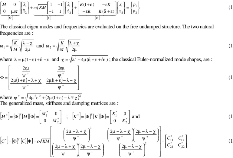
In the finite element context, the equations of motion governing the dynamics of a linear structure can be written :

[ ]{ }

M &x&+

[ ]

C

{ }

x& +

[ ]

K

{ } { }

x = p (1)

where

[ ]

M ,

[ ]

C and

[ ]

K are respectively the mass, damping and stiffness matrices.

{ }

p is the vector of the external applied loads and

{ }

x ,

{ }

x& and

{ }

x&& are the displacements, velocities and accelerations of the structural

(2)

degrees of freedom. The damping matrix is composed of different contributions : structural damping, concentrated damping and aerodynamic damping :

[ ] [ ] [ ] [ ]

C = CS + CD + CA (2)

For the big and complex structures studied in practical cases, the size N of the system (the number of degrees of freedom) can easily reach 104 to 105. It is then convenient to change the unknowns to a limited number M of modal coordinates (Clough, Penzien, 1993) :

{ }

x

[ ]

{ }

q _{x _{q M N M n s coordinate al n in s coordinate structural i = Φ << ↔ Φ =

∑

=1 mod (3)

The equations of motion become :

[ ]

_M∗

{ }

_&_q_& ₊

[ ]

_C∗

{ }

_q_& ₊

[ ]

_K∗

{ }

_q ₌

{ }

_p∗ ₍₃₎ where

[ ]

M∗ =

[ ] [ ][ ]

ΦT M Φ ,

[ ]

K∗ =

[ ] [ ][ ]

ΦT K Φ and

[ ]

C∗ =

[ ] [ ][ ]

ΦT C Φ are respectively the generalized mass, stiffness and damping matrices. Provided the classical mode shapes are used, the first two are diagonal and the equations are then coupled by the damping terms only. This is the main reason for the proportional damping which supposes that the generalized damping matrix

[ ]

C∗ is also diagonal. This hypothesis is generally adopted for the structural damping because there is not enough information about it to characterize it with a more complex law.

Concentrated and aerodynamic dampings are however characterized by precise mathematical laws. The modal damping associated with these is no longer diagonal. The generalized damping matrix

[ ]

C∗ is then a full matrix (semi-definite positive). Although the problem can be solved in the time domain, this paper will focus on a resolution in the frequency domain only. In this domain, the equations become :

[ ] [ ] [ ]

(

₋_ω2 _M∗ ₊_i_ω_C∗ ₊ _K∗

)

{ }

_Q ₌

[

_G₍_ω₎

]{ }

_Q ₌

{ }

_P∗ ₍₄₎

where

{ }

Q and

{ }

P∗ are respectively the Fourier transforms of the modal coordinates and forces. The impedance matrix

[

G(ω)

]

is defined as a function of the frequency and, because of the non proportional damping, its off-diagonal terms are not equal to zero.

The computation of the modal responses requires then now the inversion of this impedance matrix :

{ }

_Q ₌

[

_G₍_ω₎

]

−1

{ }

_P∗ ₌

[

_H₍_ω₎

]

{ }

_P∗ ₍₅₎

even though only a diagonal matrix has to be inverted when the system was uncoupled (Rayleigh structural damping only). Eqn. 5 introduces the inverse of the impedance matrix : the modal transfer matrix (

[

H(ω)

]

).

Because of the non proportional damping, it is now much more time-consuming particularly since the operation has to be repeated for each treated frequency !

Usual solutions to non proportional damping

Several solutions are generally proposed to analyze structures with non proportional damping. The adoption of one or another depends of the kind of problem to be solved.

Classical eigenmodes and full matrix problem

The first method to solve the problem was presented here above. It is not really a solution because it consists in keeping the classical eigenmodes and working on the full matrix problem which requires then the inversion of the impedance matrix. In general, this is not so important because in many engineering problems, a few modes only are sufficient to represent the general behaviour of the structure.

This solution should of course be adopted only if the size of the reduced problem is limited.

Classical eigenmodes and uncoupled problem

In a wide range of engineering problems, the off-diagonal terms are not as important as the diagonal ones. This is for example the case when the damping added by dash-pots or the aerodynamic damping is of the same order as the structural one.

(3)

In this case, engineers sometimes work with the classical mode shapes, deal with a coupled system of equations and simply drop the off-diagonal terms. The supplemental damping (coming from dash-pots and wind) is then only taken into account via its diagonal terms in the modal basis (H. A. Buchholdt, 1997).

The results obtained in this case are no longer the exact results but depend of the formulated approximations.

However, this solution is probably the best when the off-diagonal terms are small compared to the diagonal ones.

Complex eigenmodes

In an other range of problems, it is necessary to work with uncoupled equations (Oliveto G., Santini A, 1996 ). Mathematicians have then imagined to work with the complex eigenmodes. The classical ones are estimated by solving :

[ ]

(

K −ω2 M

)

{ }

Φ =0 (6)

which does not include any notion of damping at all. Unlike the classical ones, for the complex eigenmodes, the damping properties of the system are included in their determination :

[ ]

(

K −ω2 M +iωC

)

{ }

Φ_c =0 (7)

This definition leads to complex eigenmodes and eigenvalues which are of course more difficult to handle than the classical real ones. Anyway, these new modes allow to uncouple the equations of motions and make then their solution easier. However, imaginary modes remove their physical representation ; this mathematical, radical and efficient solution should be used when the off-diagonal terms of the generalized damping matrix are important compared to the diagonal ones.

Taylor series expansion

Here comes now another range of problems : the off-diagonal terms are “small”(cf § 2.2.2) but it is desired to take them into account, even in a limited way.

First of all, let us remark that for a<x, the definition of the geometric series enables to write :

        +       −       + − = + = + L 3 2 1 1 1 1 1 1 x a x a x a x x a x a x (8)

which is also the Taylor series development of the inverse of a scalar. This formula expresses the inverse of a scalar (x+a) in terms of the inverse of its neighbor (x) (because a is supposed to be small). It would be interesting to develop the same formulation for matrices. Let us split the impedance matrix in two parts :

[

G(ω)

] [

= G_d(ω)

] [

+ G_c(ω)

]

(9)

[

Gd(ω)

]

contains only the diagonal terms whereas

[

Gc(ω)

]

contains only the off-diagonal ones. For clarity in the notations, the argument will be dropped. Let us note again that :

(

1

)

1

(

1

(

)

1 1 1 1 1 − − − − − − − − ₋ ₌ ₋ ₌ ₊ ₋ ₌ G G G G I G G G G I G G G Gd d d d c d c (10)

We can then write successively :

(

1 1

)

1 1 1 1

(

1

)

1

(

1

(

1

)

1

(

1 1 1

)

1 1 − − − − − − − − − − − − − − − − ₌_G ₋_G ₊_G ₌_G ₋_G _G _G ₌_G _I₋_G_G ₌_G _I₋_G _G _I₋_G _G ₌_G _I₋_G _G ₊_G _G _G _G G _d _d _d _d _c _d _c _d _c _d _c _d _c _d _c _d _c (11) And so on, leading finally to :

(

) (

)

_    ₋ ₊ ₋ ₊ ₋ = − − − − − −₁ ₁ ₁ ₁2 ₁3 ₁4 _L d c d c d c d c d I G G G G G G G G G G (12) The modal transfer matrix

[

] [

]

1

) ( )

(ω = Gω −

H is then obtained by the sum of the transfer matrix corresponding to the uncoupled problem and successive corrections :

L + ∆ + ∆ + ∆ + ∆ + =H H1 H2 H3 H4 H _d (13) where ( )

(

)

n d c d n n G G G H = −1 −1 −1 ∆

(4)

This latter expression is the matrix equivalent of the scalar Taylor series expansion given here above.

Provided the off-diagonal terms play a secondary role in the full impedance matrix (

[

Gc(ω)

] [

<< G(ω)

]

), the

inverse of the full matrix can be estimated with a few terms, as a function of the inverse of the diagonal matrix which is really easy to compute.

The method for inverting a quasi-diagonal matrix was presented here in the context of a resolution in the frequency domain. This method should be used when computing the modal transfer matrix of the structure. Once this is done the rest of the computation is of course the same as usual.

APPLICATION TO A SIMPLE STRUCTURE

Even though the method is devoted to bigger systems, it is good to understand its efficiency on a simple structure.

The example concerns the 2-DOF structure shown in figure 1. Two degrees of freedom are coupled by a structural stiffness (εK) and by a linear dash-pot (viscosity c KM ).

Figure 1 : Sketch of the 2-DOF system Within the structural coordinates, the equations of motion can be written :

[ ] [ ] [ ]       =             + − − + +             − − +             2 1 2 1 2 1 2 1 ) ( ) 1 ( 1 1 1 1 0 0 p p x x K K K K x x KM c x x M M K C M 4 4 4 3 4 4 4 2 1 & & 4 4 3 4 4 2 1 & & & & 43 42 1 ε δ ε ε ε µ (14)

The classical eigen modes and frequencies are evaluated on the free undamped structure. The two natural frequencies are : µ χ λ ω 2 1 − = M K and µ χ λ ω 2 2 + = M K (15) where λ =µ(1+ε)+δ+ε and χ= λ2−4µ(δ+ε+δε); the classical Euler-normalized mode shapes, are :

( )

            − − + + − + = Φ + − + − ψ χ λ ε µ ψ χ λ ε µ ψ εµ ψ εµ 1 2 1 2 2 2 (16) where 2 2

(

)

2 ) 1 ( 2 4µ ε µ ε λ χ ψ±= + + − m

The generalized mass, stiffness and damping matrices are :

[ ]

[ ] [ ][ ]

        = Φ Φ = ∗ * 2 * 1 0 0 M M M M T ;

[ ]

[ ] [ ][ ]

        = Φ Φ = ∗ * 2 * 1 0 0 K K K K T and (17)

[ ]

[ ] [ ][ ]

        =                         − −         − −         − +         − −         − +         − + = Φ Φ = + + − + − − ∗ * 22 * 21 * 12 * 11 2 2 2 2 2 2 2 2 C C C C KM c C C T ψ χ λ µ ψ χ λ µ ψ χ λ µ ψ χ λ µ ψ χ λ µ ψ χ λ µ (18)

The exposed case should be seen as a worst case scenario. Indeed, for any combination of the parameters, the dash-pot provides a perfectly coherent damping :

(5)

1 * 22 * 11 * 12 ₌_± C C C (19) which means that for any diagonal terms, the off diagonal ones will be as big as they are allowed to (the existence of such a maximum comes from the definite semi positive character of the matrices).

With the notations of the previous section., we can write :

        − + − + = _* 2 2 * 22 * 2 * 1 2 * 11 * 1 0 0 ) ( M C i K M C i K G_d ω ω ω ω ω ;         = 0 0 ) ( * 21 * 12 C C i G_c ω ω (20)       =             − + − + = = − 22 11 * 2 2 * 22 * 2 * 1 2 * 11 * 1 1 0 0 1 0 0 1 d d d d H H M C i K M C i K G H ω ω ω ω ₍₂₁₎

The corrections are expressed by :

( )

(

)

( )

(

)

       =       − − =       − = ∆ ) ( 2 0 0 ) ( 1 2 0 1 1 0 * 22 11 22 11 * 12 * 22 11 * 12 * * even i n n if H H H H C odd n n n if i H H C H d d n d d n n d d n n ω ω (22)

This close form of the corrections to the diagonal transfer matrix shows that the corrections are negligible for small frequencies. The response is indeed mainly controlled by the stiffness at low frequencies. Likewise, at high frequencies, the response is mainly controlled by the mass. As the off diagonal terms are related to damping, the major modifications that the successive corrections will bring should then concern the moderated frequencies in the vicinity of the resonance peak. This statement will be clearly observable in the numerical example.

Even if damping is related to imaginary numbers, it can however affect the real part of the transfer function. It is here the case for the even corrections.

The minimum number of correction terms to keep in the development (Eqn. 22) depends on the smallness of the off-diagonal terms compared to the diagonal ones. This explains why the inversion method based on Taylor series expansions should be used in the modal coordinates only ; the off diagonal terms concerns indeed damping only.

NUMERICAL EXAMPLE

As introduced before, the efficiency of the method will be discussed on the evaluation of the transfer matrix only. The rest of the computation should happen as usual.

Let us consider the 2-DOF system presented in the previous section. The parameters will take these given values : 2 ; 5 . 0 ; 1 ; 1 = = = = K µ δ M (23)

A structural damping ξ=0.02 will also be added.

We will first consider that (a) the two degrees of freedom are completely uncoupled (ε=0;c=0) and then simultaneously re-linked via : (b) a spring only (ε=0.5;c=0) , (c) a dash-pot only (ε=0;c=0.35) and (d) a mixed solution (ε=0.5;c=0.35).

As the stiffness of the whole structure will be different from one case to another, the eigen modes will change. The comparisons will then be made on the displacements of the structural degrees of freedom (i.e. the structural transfer matrix) rather than on the modal coordinates.

The comparisons will be drawn between the norms of the elements of the transfer matrix. Three terms have then to be compared : both diagonal terms (denoted hereunder DOF 1 and DOF 2) and the off-diagonal term (denoted Coupling term).

(6)

The two degrees of freedom are completely uncoupled (ε=0;c=0)

The natural frequencies of the 2-DOF system are f1=1 rad/s and f2=2 rad/s ; the modal damping coefficient are

the structural ones (ξ1= ξ 2=0.02). The transfer functions have the usual shape with the resonance peak at the

natural frequencies of each degree of freedom. As the transfer matrix is diagonal in the modal coordinates, the exact solution is the uncoupled one. The corrections expressed by Eqn. 22 are then all zero in this particular case.

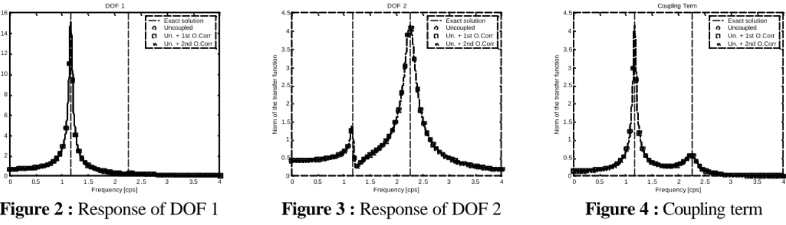
Stiff link (ε=0.5;c=0)

The eigenvalue analysis is performed on the re-linked system. As adding a rigid link between the masses contributes to adding stiffness to the whole structure, natural frequencies are then shifted up (f1=1.167 rad/s

and f2=2.267 rad/s). The modal damping coefficient remain however unchanged (ξ1= ξ 2=0.02). As the only

damping (structural damping) is proportional, the modal equations of motion are then uncoupled.

The exact solution still corresponds to the uncoupled one and the successive corrections which should be added are all equal to zero.

As the degrees of freedom are now re-linked, both diagonal terms present two resonant peaks. The first mode (the softer) is anyway not much influenced by the second one.

0 0.5 1 1.5 2 2.5 3 3.5 4 0 2 4 6 8 10 12 14 16 DOF 1 Frequency [cps]

Norm of the transfer function

Exact solution Uncoupled Un. + 1st O.Corr Un. + 2nd O.Corr

Figure 2 : Response of DOF 1

0 0.5 1 1.5 2 2.5 3 3.5 4 0 0.5 1 1.5 2 2.5 3 3.5 4 4.5 DOF 2 Frequency [cps]

0 0.5 1 1.5 2 2.5 3 3.5 4 0 0.5 1 1.5 2 2.5 3 3.5 4 4.5 Coupling Term Frequency [cps]

Figure 4 : Coupling term The off diagonal term in the modal transfer function is still equal to zero (because the eigenvalue analysis has been performed on the system linked with a spring). But, when projected back to the structural coordinates, there is a coupling term which also present resonant peaks. By definition, this term represents the displacement at DOF 1 when forces are applied at DOF 2 and vice versa.

Viscous link (ε=0;c=0.35)

When as purely viscous link is added between the two masses, the natural frequencies of the structure are not affected (f1=1 rad/s and f2=2 rad/s) but the modal damping coefficients are increased (ξ1= ξ 2=0.195). The

positions of the resonant peaks seem to be changed ; this is a consequence of high damping coefficients.

0 0.5 1 1.5 2 2.5 3 3.5 4 0 0.5 1 1.5 2 2.5 3 DOF 1 Frequency [cps]

0 0.5 1 1.5 2 2.5 3 3.5 4 0 0.2 0.4 0.6 0.8 1 1.2 1.4 DOF 2 Frequency [cps]

0 0.5 1 1.5 2 2.5 3 3.5 4 0 0.1 0.2 0.3 0.4 0.5 0.6 0.7 Coupling Term Frequency [cps]

Exact solution Uncoupled Un. + 1st O.Corr Un. + 2nd O.Corr Un. + 3rd O.Corr

Figure 7 : Coupling term Figures 5 and 6 show that for the highly damped structure (ξ ~ 20 %), and for an unfavorable distribution of the viscous effect, a second order approximation gives already good results.

For the softer DOF, the approximation gives very good results and for the second one the estimated values are smaller in the vicinity of the resonant peak and larger for higher frequencies. Compared to the exact solution and in terms of integral of the norm of the transfer function, there is a difference of 0.6 % only. This means

(7)

that the total energy will be correctly estimated but not perfectly distributed in the frequency range (lower moments will be better approximated than higher ones).

As the link is now purely viscous, neglecting the off diagonal terms results in no structural coupling at all. As modal and structural basis corresponds, it can be shown easily that odd corrections contribute to the coupling term while even corrections concern the diagonal terms only.

Concerning this coupling effect, the second order approximation will give the same result than the first order one, i.e. a difference of about 11 % on the integral. Depending upon the problem to be solved, this approximation can be accurate enough or not. It should be kept in mind that this method has been imagined to give a fast (and then less accurate) result. It allows at least to estimate the coupling term ! Anyway, a third correction term could be taken into account which would reduce the difference to less than 0.5 %.

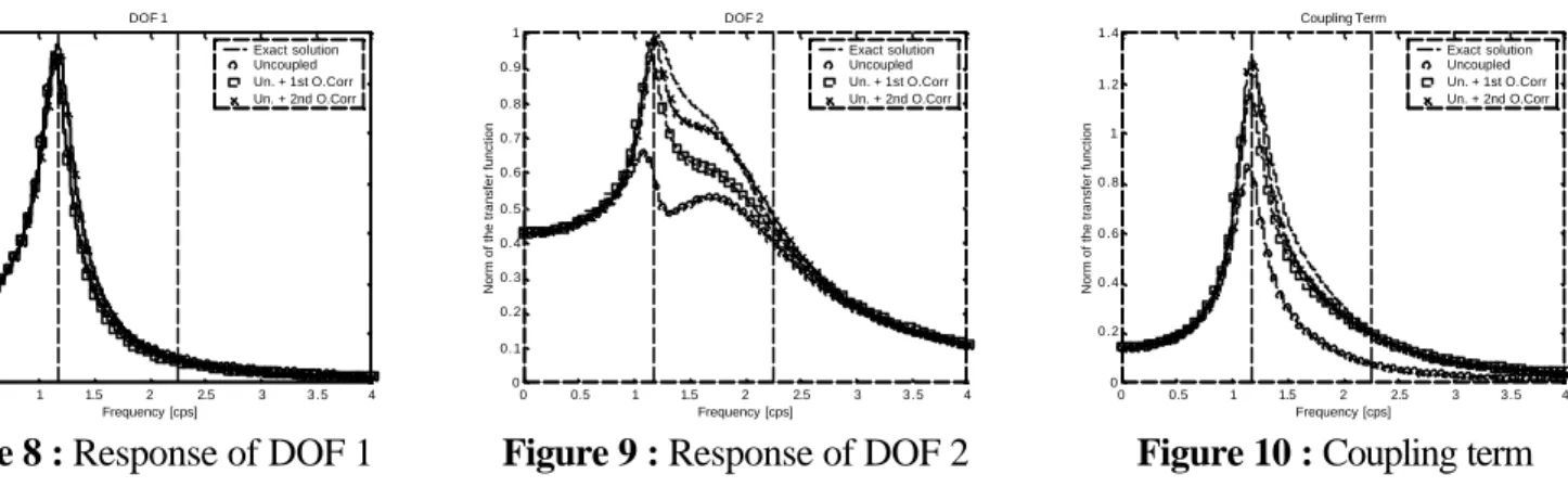
Hybrid link (ε=0.5;c=0.35)

When both masses are linked with a spring and a dash-pot, natural frequencies and modal damping coefficients are both affected : f1=1.167 rad/s ; f2=2.267 rad/s ; ξ1=0.096 ; ξ 2=0.2125.

This solution is of course more likely to be experienced in practical cases. The eigen modes do not correspond to one or another mass vibrating alone anymore but rather to the piles vibrating in phase (mode 1) or 180° out-of-phase (mode 2). It is then obvious for the second mode to be more damped than the first one.

Figures 8 and 9 show that the unilateral responses of the degrees of freedom are well estimated. For the second order correction method, the difference is 3 % only for the second degree of freedom.

0 0.5 1 1.5 2 2.5 3 3.5 4 0 0.5 1 1.5 2 2.5 3 3.5 DOF 1 Frequency [cps]

0 0.5 1 1.5 2 2.5 3 3.5 4 0 0.1 0.2 0.3 0.4 0.5 0.6 0.7 0.8 0.9 1 DOF 2 Frequency [cps]

0 0.5 1 1.5 2 2.5 3 3.5 4 0 0.2 0.4 0.6 0.8 1 1.2 1.4 Coupling Term Frequency [cps]

Figure 10 : Coupling term The coupling term is also very well estimated with the second order approximation. The difference with the exact solution is 0.34 % only ! For this term, figure 10 indicates that the exact solution is overestimated in the vicinity of the peak and underestimated for higher frequencies.

PERFORMANCE TEST

Another series of computation has been performed in order to determine the relative errors as a function of the modal damping coefficients. In order to represent a worst case scenario, the structural damping is set equal to zero. Furthermore, in order to have the same damping coefficient for each mode, the link is supposed to be perfectly viscous. We have just seen that this situation is the most unfavorable one.

0 0.05 0.1 0.15 0.2 0.25 0.3 -10 -8 -6 -4 -2 0 2 DOF 1 ξ Relative error [%] 1st order 2nd order

0 0.05 0.1 0.15 0.2 0.25 0.3 -10 -8 -6 -4 -2 0 2 DOF 2 ξ Relative error [%] 1st order 2nd order

0 0.05 0.1 0.15 0.2 0.25 0.3 -10 -8 -6 -4 -2 0 2 Coupling Term ξ Relative error [%] 1st order 3rd order

(8)

The use of Taylor series approximations for the computation of modal transfer functions with coupled modes is the most effective when the first order correction only is sufficient. From the worst case described here over, it can be seen that for damping coefficients up to 12 %, the errors committed on the integral of the norm of the transfer function are smaller than 5 %. Concerning the coupling terms, the error is a little bit higher but the coupling effects are anyway taken into account.

If the modal damping was still higher, it should be recommended to add also the second correction term. This is not a problem in itself but reduces the efficiency of the method which should optimally work with one correction only.

If the modal damping was even more important, a third order correction method could be employed but the time spent in inverting the impedance matrix (to have then the exact result) could become competitive compared to the time needed to compute and add the first three correction terms.

CONCLUDING REMARKS

From inverting a full matrix to making use of the complex eigen modes, several solutions are generally proposed to treat non proportional damping. The choice of one or another method depends on the damping characteristics.

This paper has presented a method based on Taylor polynomial approximations. It proposes to compute the actual transfer matrix by adding correction terms to the transfer matrix obtained with the diagonal terms only. The method requires then neither matrix inversion nor estimation of complex eigen modes.

The method turns the analysis to its advantage when the structure needs many eigen modes to be represented correctly and when the modal off diagonal terms play a secondary role.

Even though it should be applied to big structures, the method has been applied here to a very simple one in order to show its efficiency.

Generally speaking the method is very efficient when one correction term is enough to represent correctly the behaviour of the structure. For a worst case scenario considered on the simple structure, the method gives accurate results for damping coefficients up to 12%.

The application range of the method is very wide. It concerns indeed the computation of the transfer matrix which is necessary for any analysis in the frequency domain. Furthermore, it could also be applied in a time domain analysis where an inversion of a quasi-diagonal matrix is also required.

REFERENCES

Buchholdt, H. A. (1997). Dynamics of the structures. London : Thomas Telford Publications Clough, R. W., Penzien J. (1993). Dynamics of structures. Mc Graw-Hill Book Co.

Oliveto G., Santini A. (1996). Time domain response of a one-dimensional soil-structure interacting model via complex analysis, Engineering Structures, Volume 18, Issue 6, June 1996, Pages 425-436