Towards coordination algorithms on compact Lie groups
Alain Sarlette
Supervisor: Rodolphe Sepulchre
DEA research report 2007
Department of Electrical Engineering and Computer Science
University of Li`ege
Acknowledgments
Hearty thanks are due to Professor Rodolphe Sepulchre, whose enthusiasm, clarifying ideas and support beyond the strict limits of a supervisor, played a major role towards the completion of the present work. Further, Professor Naomi Leonard and the Mechanical and Aerospace Engineering department of Princeton University are acknowledged for an - in all respects - enriching research visit of 3 months. Further thanks go to the many people who have shared insightful discussions. Dr. Luca Scardovi and Professor Pierre-Antoine Absil were the most frequent collaborators. All these people, including colleagues at Li`ege University and Princeton University, also deserve many thanks for all their friendship. As always, the support of the family was crucial. Finally, it must be mentioned that this work was achieved with the financial support of the FNRS (National Fund for Scientific Research) and the Belgian Network DYSCO (Dynamical Systems, Control, and Optimization) funded by the Interuniversity Attraction Poles Programme, initiated by the Belgian State, Science Policy Office.
Abstract
The present work considers the design of control algorithms to coordinate a swarm of identical, autonomous, cooperating agents that evolve on compact Lie groups. The objective is that the agents reach a so-called consensus state without using any external reference. In the same line of thought, a leader-follower approach where ’follower’ agents would track one ’leader’ agent is excluded, in favor of a fully cooperative strategy. Moreover, the presence of communication links between agents is explicitly restricted, leading to undirected, directed and/or time-varying com-munication structures.
Two levels of complexity are considered for the models of the agents. First, they are modeled as simple integrators on Lie groups. This setting is meaningful in a trajectory-planning context for swarms of mechanical vehicles, or to solve algorithmic problems involving multiple agent coor-dination. In a second step, the model of Newtonian mechanics is used for Lie group solids, which correspond to the abstraction of the Euler laws for the rotation of a rigid body to general Lie groups. This setting is relevant for the actual control of mechanical vehicles through torques and forces.
As a common starting point, the consensus problem is formulated in terms of the extrema of a cost function. This cost function is linked to a specific centroid definition on manifolds, which is referred to in this work as the induced arithmetic mean, that is easily computable in closed form and hence may be of independent interest. Using the integrator model, this naturally leads to efficient gradient algorithms to synchronize (i.e. maximizing the consensus) or balance (i.e. minimizing the consensus) the agents; the latter however can only implement the corresponding control laws if the communication graph is fixed and undirected. For directed and/or varying com-munication graphs, a convenient adaptation of the gradient algorithms is obtained using auxiliary
estimator variables that evolve in an embedding vector space. An extension of these results to
homogeneous manifolds is briefly discussed. For the mechanical model, the coordination objective is specialized to coordinated motion (i.e. moving such that the relative positions of the agents are conserved) and synchronization (i.e. having all the agents at the same position on the Lie group). Control laws are derived using two classical approaches of nonlinear control - tracking and energy shaping. They are both based on the ideas developed in the first part.
For the sake of easier understanding and given its practical importance as representing orien-tations of rigid bodies in 3-dimensional space, the group SO(3) (or more generally SO(n)) is used as a running example throughout this report. Other examples are the circle SO(2) and, for the extension to homogeneous manifolds, the Grassmann manifolds Grass(p, n).
As this report is written in the middle of research activities, it closes with several future research directions that can be explored in the continuity of the present work.
Contents
Overview of the contributions 5
1 Relevance of coordination on Lie groups 7
1.1 Applications involving coordination on compact Lie groups . . . 7
1.2 Previous work . . . 8
1.2.1 Algorithmic consensus . . . 9
1.2.2 Coordination of mechanical systems . . . 10
2 Theoretical background 11 2.1 Elements of graph theory . . . 11
2.2 Systems on compact Lie groups and homogeneous manifolds . . . 12
2.2.1 Motion on Lie groups and homogeneous manifolds . . . 12
2.2.2 Dynamics on compact Lie groups . . . 14
2.2.3 Examples . . . 14
3 Induced arithmetic mean and consensus reaching on Lie groups 17 3.1 The induced arithmetic mean . . . 17
3.1.1 Definition and discussion . . . 17
3.1.2 Examples . . . 19
3.2 Consensus as an optimization task . . . 20
3.2.1 Definition . . . 20
3.2.2 Examples . . . 22
3.2.3 Consensus optimization strategy . . . 22
3.2.4 Example . . . 24
3.3 Gradient consensus algorithms . . . 24
3.3.1 Gradient algorithms for fixed undirected graphs . . . 24
3.3.2 Extension to directed and time-varying graphs . . . 25
3.3.3 Examples . . . 26
3.4 Consensus algorithms with estimator variables . . . 28
3.4.1 Synchronization algorithm . . . 28
3.4.2 Anti-consensus algorithm . . . 29
3.4.3 About the communication of estimator variables . . . 31
3.4.4 Example . . . 31
3.5 Extension to homogeneous manifolds . . . 32
3.5.1 Example . . . 33
4 Synchronization of autonomous Lie group solids 36 4.1 Problem setting . . . 36
4.2 Coordination strategy . . . 37
4.2.1 From integrators to mechanical systems . . . 37
4.2.2 Example . . . 39
4.3 Consensus tracking . . . 39
4.3.1 Basic considerations . . . 39
4.3.2 The computed torque method . . . 40
4.3.3 The high gain method . . . 42
4.3.4 Example . . . 44
4.4 Energy shaping . . . 44
4.4.1 Dissipation in inertial space . . . 45
4.4.2 Dissipation in shape space . . . 46
Finale 51 Recap - Overview of the contributions revisited . . . 51 Conclusions . . . 52 Perspectives for future research . . . 52
Overview of the contributions
The work presented in this report is part of a larger research project on coordinated motion control on Lie groups. The present work, as a first step, is restricted to compact Lie groups. The starting point is a swarm of identical agents, moving autonomously on a compact Lie group G. The indi-vidual agents can share information along communication links as defined by an interconnection graph. The task is to design control laws for the agents as a function of the relative positions of connected agents, such that they move in order to reach a state of coordinated motion. These control laws may imply no external reference, and the various possibilities that must be consid-ered for the interconnection graph exclude a leader-follower approach. The strategy behind the algorithms embeds G in a Euclidean space E. Distances between agents are measured in E in order to build cost functions for an optimization-based approach. Two types of models of increasing complexity are considered for the (always fully actuated) agents: simple integrators and controlled mechanical systems (so-called Lie group solids).
The simple integrator model is used to focus on the issues related to systems that are globally distributed on a Lie group and to reduced interconnections in this setting. The main contribution is to define various qualitative situations for the relative positions of the agents on the Lie group
G. In this first part, the degree of freedom concerning possible synchronized motions of the agents
is not considered: the algorithms drive the agents towards a specific configuration where they remain at rest. The two extreme such configurations are the situation where all the agents are at the same position (synchronization) and the situation where the agents are spread in some way on the whole manifold (balancing). Those two problems are formulated as optimizing (i.e., maximizing or minimizing) a simple consensus function which depends on the relative states of all the pairs of agents. Using a similar characterization but with a limited set of agent pairs, intermediate situations called consensus and anti-consensus are defined. Those are all built on a specific definition of the mean of positions on a manifold, which may be interesting on its own account. It is called the induced arithmetic mean in the present paper.
Two types of algorithms are proposed, depending on the goal and the available communication links. For fixed undirected interconnection graphs, gradient algorithms can be used to lead the agents to corresponding consensus or anti-consensus states. For time-varying and/or directed interconnection graphs, the two extreme cases of synchronization and balancing can be reached thanks to an adaptation of the previous algorithms using auxiliary estimator variables.
These results can be generalized to connected compact homogeneous manifolds. A journal paper version of this first part of the report can be found in [1].
The second part of the report merges the consensus approach considered in the first part with the more realistic model of a mechanical system moving on a Lie group. The main contribution here is the design of algorithms such that the swarm converges towards synchronization of the positions or to synchronization of the velocities (such that the relative positions remain constant). In both cases, the control laws explicitly incorporate the possibility to have a (non-trivial) synchronized motion of the agents. The algorithms are derived using two popular strategies in control of mechanical systems: (consensus) tracking and energy shaping.
For the consensus tracking approach, the trajectories resulting from the consensus algorithms as designed in the first part are considered as desired trajectories that each mechanical agent asymptotically tracks. Though an integrated proof is provided for particular tracking controllers, any controller developed for tracking (or, with some restrictions, even for stabilization) on Lie groups can probably be used instead.
For the energy shaping approach, the consensus function defined in the first part is used as an artificial potential for the mechanical system. This approach is not entirely new, but it seems that the proper design of dissipation in order to obtain asymptotic stability of the synchronized state, without using an external reference for the swarm, had not been explicitly solved yet at the time
of the research presented in this report.
The results in this part could not all be formulated for general connected compact Lie groups: the last result is specialized to the classical (and probably most useful) Lie group SO(3), for which the “Lie group solid” becomes the actual 3-dimensional rotating rigid body. A conference paper version of this second part of the report, specialized to SO(3), can be found in [2].
Though the subjects and approaches in this work are popular in the literature, very few au-thors to date solved relevant problems on Lie groups. Among the many challenges that Lie groups raise with respect to vector spaces, the most significant are the non-convexity of the state space (leading to non-convex problems as soon as the agents are spread over a large portion of the state space - see the contributions in the first part of this report) and the particular relations between position, velocity and acceleration (leading among others to drift terms in the mechanical models - see the contributions in the second part of this report).
The report is organized as follows. The relevance of the present work is briefly discussed in Section 1, including some considerations about previous work. Section 2 provides the necessary background and notations for the mathematical formulations and developments in the main part of the report. Section 3 contains the first part of the main contributions, in which the simple integrator model is considered in order to define the induced arithmetic mean, consensus and anti-consensus configurations, and deduce algorithms to drive the swarm of simple integrators towards these configurations. Section 4, containing the second part of the main contributions, goes one step further by considering mechanical models and synchronized motions of the swarm. After summarizing the results and giving some general conclusions, the report ends with a discussion about future research.
1
Relevance of coordination on Lie groups
1.1
Applications involving coordination on compact Lie groups
The distributed computation of means/averages/centroids of datasets (in an algorithmic setting) and the synchronization of a set of agents (in a control setting) - i.e. driving all the agents to a common position in state space - are ubiquitous tasks in current engineering problems. Likewise, spreading a set of agents in some optimal way in the available state space - linked to balancing as defined in the present work - is a classical problem of growing interest. Swarms of autonomous agents are increasingly considered as an advantageous option to carry out complex tasks which would be lengthy or infeasible for a single agent.
For instance, many modern space mission concepts involve the use of multiple satellites flying in formation. Mostly, the objective is to get (virtual) structures in orbit that are substantially larger than what current launch technologies can directly handle. Potential applications arising in current studies include resolution enhancement through multiple-spacecraft SAR (the InSAR concept, or ONERA’s Romulus study), interferometry (ESA’s Darwin project, NASA’s equivalent Terrestrial Planet Finder project or NASA’s Constellation-X project) or supersized focal length (ESA’s XEUS project, derived from the Symbol-X concept of CNES), sensitivity increasing through screens on secondary spacecraft (the American New World Discoverer concept for the JWST) or large-scale measurements (the ESA-NASA cooperative mission LISA), and autonomous in-orbit assembly of large real structures (projects are still at a draft level; see [3] and [4] for example). Other advantages of spacecraft formations are their robustness with respect to single spacecraft failure, and the reconfigurability of the swarm to fit specific observation requirements.
Similar lists of projects can be made for formations of unmanned aerial vehicles (UAV’s), au-tonomous underwater vehicles (AUV’s) or terrestrial platoons - in fact any type of general vehicle formations ([5, 6, 7, 8, 9, 10, 11, 12, 13, 14, 15, 16, 17, 18, 19, 20, 21, 22, 23, 24, 25, 26, 27] and references therein). A central problem in formation control is to ensure proper coordination of the agents, i.e. to bring them to and keep them in the desired formation. This requires to design coordination algorithms for mechanical systems, as is done in Section 4. At this point, it must be emphasized that accurate formation control poses several different problems of which the present work just considers one part: focusing on convergence from states that can be far away from the desired equilibrium and inherently including strong robustness considerations, the developed control laws might most probably be useful for initial deployment of the formation or for recovery after strong transient perturbations. In general, most theoretical studies are far from final science operations requirements, where accuracy is a key issue for navigation and control and unmodeled disturbances or constraints are present. An example of a practical GNC implementation for the Darwin mission can be found in [28].
The first part of this work considers coordination algorithms for simple integrators. From this algorithmic point of view, practical applications involving coordination include distributed decision making (e.g. [29, 30]), neural and communication networks (e.g. [31, 32]), clustering and other reduction methods (e.g. [33]), optimal covering or coding (e.g. [34, 35, 36, 37]) and many other fields where “dynamically computing an average” or “optimally distributing a set of points” appear as sub-tasks ([38]). In addition, in a modeling framework, the understanding of synchronization or more generally swarm behavior using simple models has led to many important studies discovering fundamental properties (e.g. [39, 40, 41]). Moreover, as is done in the present work, coordination algorithms for simple integrators can be used - more or less directly - at a task planning level for motion coordination in a swarm of mechanical systems ([13, 18, 16, 19, 42]).
Consensus algorithms are well understood in Euclidean spaces (see e.g. the results in [43, 44, 30, 29]). They are based on the natural definition and distributed computation of the centroid in such spaces. The literature about formation control of mechanical systems on vector spaces
is even wider; a thorough survey would require a longer discussion and the interested reader is referred to citations in the references of the present paper. However, as evidenced by the above list, many interesting applications involve manifolds that are not homeomorphic to a Euclidean space. Even for formations moving in R2 or R3, the orientation of the agents is characterized by
state variables in a non-Euclidean manifold SO(2) ∼= S1or SO(3). However, much less studies are
devoted to consensus and coordination on non-Euclidean spaces. For example, position control of spacecraft formations has attracted many studies, while attitude control has been addressed only in a few papers (see the following review of previous work). Balancing algorithms only make sense on compact state spaces; though many theoretical results concern convex or star-shaped subspaces of a Euclidean space (see e.g. [37]), again most interesting applications involve compact manifolds. The study of global synchronization or balancing in non-Euclidean manifolds is not widely covered in the literature - except for the circle. The definition and computation of centroids on manifolds is also scarcely addressed.
Synchronization on non-Euclidean manifolds raises particular questions that must be solved on the way to particular applications ([45, 46]). The first studies of coordination on manifolds are concerned with the circle ([13, 14, 15, 47]), a basic interest being among others the study of oscillator synchronization through the celebrated Kuramoto model ([39, 48]). The next most im-portant class of examples is probably SO(n), representing the orientations of n-dimensional rigid bodies ([7, 10, 11, 49, 50, 51]). On the algorithmic side, data fusion also considers SO(n), as well as the Grassmannian manifolds Grass(p, n) of p-dimensional subspaces in an n-dimensional space. Optimal packing often considers the sphere and Grass(p, n) as well. For instance, in [36], optimal placement of N laser beams for cancer treatment and the representation of multi-dimensional data on a 2-dimensional computer screen by means of projections on N representative planes are mentioned as practical applications of optimal distribution on Grass(p, n). Clustering algorithms on Grass(p, n) have also received attention recently [33]. The sphere and Grass(p, n) are not Lie groups, but belong to a very close family of perfectly symmetric state spaces called
homoge-neous manifolds (the manifolds corresponding to Lie groups are also termed principal homogehomoge-neous manifolds) to which the results of the first part can be more or less readily generalized.
To avoid lengthy reformulations, the present paper makes the choice to work exclusively in continuous-time. For algorithmic applications, it is perfectly legitimate to argue that a time approach would be more appropriate. The adaptation of the present algorithms to discrete-time is expected to cause no fundamental problems. For the circle, equivalent continuous-discrete-time and time algorithms are explicitly established and studied in [47]. See also [52] for discrete-time algorithms on manifolds.
1.2
Previous work
A favorite application of coordination on compact Lie groups, which also serves as the running example in the present work, is the group SO(3) characterizing the orientations of rigid bodies in 3-dimensional space. Though the present work takes an inherently geometric viewpoint of SO(3), it must be stressed that the most popular representation of rigid body orientations, particularly for applications to satellite control, uses unitary quaternions ([6, 27, 42]). The manifold corresponding to unitary quaternions is not strictly equivalent to SO(3). For individual satellite control, some easy tricks allow to tackle this problem. However, it is not clear how these tricks could be adap-tated to synchronization of autonomous satellites without using an external reference. Therefore, the quaternion representation of rigid body orientation is ignored in the present work.
1.2.1 Algorithmic consensus
A first class of previous work in the area of coordination on Lie groups concerns consensus
al-gorithms. In this approach, the agents are modeled as first- or second-order integrators whose
inputs must be designed under imposed communication constraints. The focus lies on the latter and dynamical issues are ignored and mostly irrelevant because the algorithms operate in a com-putational or task-planning framework. Most existing consensus results are valid for Euclidean state spaces ([16, 20, 21, 30, 29, 43, 44, 53, 54]), but recent work also considers non-Euclidean spaces ([12, 13, 14, 15, 22, 38, 47, 1],...).
Most of the work related to consensus on manifolds has been done on the circle S1. The
most extensive literature on the subject derives from the Kuramoto model (see [48] for a review). Recently however, synchronization on the circle has been considered from a control perspective, where the state variables represent the directions of motion of agents in the plane. Most results concern local convergence properties [16, 43]. An interesting set of globally convergent algorithms in SE(2) = S1× R2is presented in [13], but they require all-to-all communication. Some problems
related to global discrete-time synchronization on S1 under different communication constraints
are discussed in [55], where connections of the control problem with various existing models are made. Stronger results are presented in [47] for global synchronization and balancing on S1with
varying and directed communication graphs, at the cost of introducing an auxiliary estimator variable that communicating agents must exchange. Finally, [14] presents results on SE(2) similar to those of [13] but under relaxed communication assumptions, using among others the estimator strategy of [47],[38]. In [56], an algorithm similar to the basic algorithm of [13] is proposed for spheres Sn−1 ∈ Rn of arbitrary dimensions; convergence results however are still limited to the
case of S1.
Synchronization or balancing on a manifold M is closely related to the definition and compu-tation of a mean or centroid of points on M. This basic problem has attracted somewhat more attention, as can be seen from [57, 58, 45] among others.
The key element in the strategy developed in the first part of this work is the embedding of M in a Euclidean space E and the consequent easy computation of a centroid in E. This idea is not entirely new. It is connected to the “projected arithmetic mean” defined in [46] for SO(3), which similarly uses the metric of the embedding space instead of the inherent Riemannian metric along the manifold. In fact, this simplification process of computing statistics in a larger and simpler embedding manifold (usually Euclidean space) and projecting the result back onto the original manifold, goes back as far as 1972 [59].
A remark about the computation of a “centroid of subspaces” is presented in [60] as a short example, without much theoretical analysis. In fact, one observes that the algorithms of the present work, when written on Grass(p, n), are similar and can eventually be viewed as generalizing the developments in [60] in the framework of consensus and synchronization. More recently, [33] uses the embedding of Grass(p, n) with the projector representation and the associated centroid definition, exactly as is done in Section 3.5 below but without going into theoretical details, to compute the centers of the clusters in a clustering algorithm. The distance measure associated with this centroid on Grassmann is called the chordal distance in [35]; the latter notion is in fact introduced in [36] where the projector representation of Grass(p, n) and the associated distance measure in the embedding Euclidean space are used to derive optimal distributions (“packings”) of N agents on some specific Grassmann manifolds.
Finally, in general, the optimization-based design of algorithms on manifolds is a topic that has considerably developed over the last decades (see e.g. [61], [62] and the books [63, 52]).
1.2.2 Coordination of mechanical systems
A second viewpoint on coordination comes from the field of control of mechanical systems. In this framework, the non-trivial second-order dynamics on Lie groups are always explicitly incorporated. The main example used in the present work - rigid body attitudes on SO(3) - is also the most popular Lie group in the literature about mechanical systems. In a coordination framework, it has attracted some attention for its application to satellite attitude synchronization.
Algorithms that asymptotically stabilize synchronized satellite attitudes are presented in [6] and [27]. Interconnections among satellites are limited, and convergence is proven for a behavioral algorithm combining tracking of a desired attitude, eigenaxis rotations and synchronization of the swarm. However, these results strongly depend on the tracking of a common external reference: when the latter is suppressed, the limited basin of attraction from which synchronization is guar-anteed vanishes to the empty set. The work in [26, 27] similarly depends on an external reference. In [49] and [42], attitude synchronization is considered with a leader/follower approach. In that case, the leader spacecraft can be seen as a reference which is tracked by the followers. Control algorithms are presented that globally stabilize attitude synchronization, but the robustness of this approach critically depends on the reliability of the leader spacecraft and on the ability of all the followers to track it.
In these approaches, the use of the convenient but non-unique quaternion representation for rigid-body orientations can produce unwanted artefacts in the satellites’ motions: sometimes a satellite that has an attitude very close to the leader moves in the opposite direction to come back from another side. It seems that quaternions are absolutely reliable as long as relative orientations are considered individually, but can run into problems when several orientations are combined without a common external reference. Tracking algorithms working inherently on the relevant manifold (SO(3) in the present case) are developed in [50].
The authors in [7] consider the attitude synchronization problem on SO(3) without external references and quaternion artefacts. In fact, their artificial coupling potentials are the same as in the present work. Using the Method of Controlled Lagrangians, local stability of a synchronized state is studied and achieved in a specific situation (final synchronized rotation around the short principal axis, specifically fixed communication interconnections). In addition to being local, this result is not asymptotic, meaning that the satellites remain close to the equilibrium but do not converge towards it. In the same line of work ([5, 8, 9, 10, 11, 64]), asymptotic convergence is achieved by adding an external reference. Thanks to their close link to the present study, these contributions are discussed in more detail in Section 4.2.
It must be mentioned that powerful theoretical tools have been developed to study highly symmetric mechanical systems, though their use is avoided in the present work because of their difficulty of application in practice. The starting point for these developments is a classical tool which is indeed used in the present work: energy shaping1. Building on these energy methods,
various reduction techniques serve to deal with the symmetries of the systems themselves and those arising from their interconnection. Relevant tools are the Energy-Momentum ([65]) and Energy-Casimir ([66]) methods as well as Semidirect Product Reduction [67]. Application of these concepts to coordination of multiple agents is discussed in [68].
2
Theoretical background
The present section briefly reviews two key mathematical tools that are needed to understand the core of the work. First, the representation of agent interconnections by graphs is clarified. Sec-ondly, a technical section about Lie groups and homogeneous manifolds provides an introduction to their basic properties and reviews some identities that are used in the sequel.
2.1
Elements of graph theory
Coordination in a group of agents depends on the available communication links. When considering limited agent interconnections, it is customary to represent the communication links by means of a graph. The graph G is composed of N vertices (denoting the N agents) and contains the edge (j, k) if agent j sends information to agent k (i.e. vertex j is an in-neighbor of vertex k), which is denoted j à k. A positive weight ajkis associated to each edge (j, k) to obtain a weighted graph;
the weight is extended to any pair of vertices by imposing ajk = 0 iff (j, k) does not belong to
the graph edges of G. The full notation for the resulting digraph (directed graph) is G(V, E, A) where V denotes the set of vertices, E denotes the set of edges and the matrix A, composed of the elements ajk, is called the adjacency matrix of the graph. In agreement with the representation
of communication links, it is assumed that akk= 0 ∀k.
The out-degree of a vertex k is defined as the quantity d(o)k = PNj=1akj of information that
leaves k towards other agents and the in-degree of k is the quantity d(i)k =PNj=1ajkof information
that k receives from other agents. These degrees can be assembled in diagonal matrices D(o)
and D(i). A balanced graph is a graph for which D(o) = D(i). This is satisfied in particular by
undirected graphs, for which A = AT. A graph is called bidirectional if (j, k) ∈ E ⇔ (k, j) ∈ E
(but not necessarily A = AT).
The Laplacian L of a graph G is defined as L = D − A. Some variations exist on which degree to use for D in the case of directed graphs; to avoid confusion, one can define the in-Laplacian
L(i) = D(i)− A and the out-Laplacian L(o) = D(o)− A. By construction, L(i) has zero column
sums and L(o) has zero row sums. The spectrum of the Laplacian reflects several interesting
properties of the associated graph, specially in the case of undirected graphs (see for example [69]). A fundamental property is that the Laplacian of an undirected graph has non-negative eigenvalues, the zero eigenvalues corresponding exactly to the different connected components of
G.
A digraph G(V, E, A) is strongly connected if there is a directed path from any vertex j to any vertex l (i.e. a sequence of vertices starting with j and ending with l such that (vk, vk+1) ∈ E for
any two consecutive vertices vkand vk+1); if there is such a path in the associated undirected graph,
derived from the adjacency matrix A + AT, then G is weakly connected. A connected component
of a disconnect graph G is a subset of nodes such that, together with the edges connecting them in G, they form a connected graph.
When considering time-varying interconnections, a time-varying graph G(t) is used and all the previously defined elements simply depend on time. Infinitesimally shortly lasting edges can be avoided by requiring the graph to be piecewise continuous. Another frequent requirement in this line of thought is that the elements of A(t) must be bounded and satisfy some threshold
ajk(t) ≥ δ > 0 ∀(j, k) ∈ E(t) and ∀t. A graph G(t) satisfying these assumptions is called a
bounded δ-digraph. The present paper always considers piecewise continuous, bounded δ-digraphs.
there is a path from j to k for the digraph ¯G(V, ¯E, ¯A) defined by ¯ajk = ( Rt2 t1 ajk(t)dt if Rt2 t1 ajk(t)dt ≥ δ 0 if Rt2 t1 ajk(t)dt < δ (j, k) ∈ ¯E iff ¯ajk6= 0 .
A δ-digraph G(t) is called uniformly connected if there exist a vertex k and a time horizon T > 0 such that ∀t, k is connected to all other vertices across [t, t + T ].
2.2
Systems on compact Lie groups and homogeneous manifolds
The present section only briefly reviews some elements related to Lie groups and homogeneous manifolds, mainly for the purpose of defining the notation used and recalling some key properties used later in this work. It contains no formal definitions nor proofs, as the reader is expected to be familiar with the subject. References about Lie groups abound and, if necessary, it should be possible to review the basics that are required to understand the following report in any of them.
2.2.1 Motion on Lie groups and homogeneous manifolds
Compact Lie groups The present report considers a swarm of N agents that evolve on a connected compact Lie group G. The position of agent k on G is denoted by yk. The basic
operation on a Lie group G is the group multiplication ykyj. The group also contains a special
identity element e such that e yk = yke = yk and an inverse element y−1k for each yk such that
yk−1yk = yky−1k = e. However, when considering the manifold associated to the Lie group G, it
seems intuitively meaningless to “multiply” (or, thinking as on a vector space, to add) two positions in physical space; multiplication (or addition) of two positions would only make sense if a fixed reference (like the identity e) was explicitly present. The present work precisely wants to avoid the use of any fixed reference. Therefore, group multiplications should not involve actual positions but only relative positions, i.e. the multiplication yk(yk−1yj) is admitted but the multiplication
ykyj is not. In some sense, the agents evolve on “a Lie group on which the reference e has been
deleted”2. In practice, the conclusion of this paragraph should simply be that, though Lie groups
usually contain a reference point e and allow multiplication of 2 absolute positions, in the present work the use of a fixed reference is not admitted and everything is formulated in terms of relative positions. Mathematically, this may be formalized by requiring that the behavior of the system remains unchanged if all the agent positions are translated (i.e. multiplied) by the same arbitrary
g ∈ G. Expressions that are invariant with respect to such a translation will be called shape entities.
Elements of a Lie group are usually represented as invertible matrices. The basic representation of a Lie group is the adjoint representation. An important property of compact Lie groups is that their adjoint representation is always unitary, i.e. the matrices yk representing the elements yk
of G are unitary. For the ease of notation, the present report always assumes real matrices; the formulation for complex Lie groups is straightforwardly obtained by expliciting the real and imaginary parts of each complex number. The matrices representing positions on G are thus orthogonal, and as G must be connected, it can be assumed without loss of generality that they belong to the matrix group SO(n). But one should not be mistaken to simply work on G ∼= SO(n) - indeed, in general G could be any subgroup of SO(n).
2Formally, this actually means that the agents evolve on the principal homogeneous manifold associated to the
Lie group G. The term “Lie group” has been preferred to “principal homogeneous manifold” in the present report because Lie groups are much more popular and the only difference, explained in this remark, can easily be taken into account explicitly.
The tangent space T Geat the origin (and actually at any point) of a group G is a vector space.
This vector space can be turned into a Lie algebra g by defining a Lie bracket [·, ·] : T Ge× T Ge→
T Gewhich must satisfy the following properties.
• Bilinearity: [aξ1+ bξ2, ξ3] = a[ξ1, ξ3] + b[ξ2, ξ3] and [ξ3, aξ1+ bξ2] = a[ξ3, ξ1] + b[ξ3, ξ2] for all
ξ1, ξ2, ξ3∈ g and a, b ∈ R.
• Skew-symmetry: [ξ1, ξ2] = −[ξ2, ξ1] for all ξ1, ξ2∈ g.
• Jacobi identity: [ξ1, [ξ2, ξ3]] + [ξ2, [ξ3, ξ1]] + [ξ3, [ξ1, ξ2]] = 0 for all ξ1, ξ2, ξ3∈ g.
Another important property of the Lie bracket on compact Lie groups is that [ξ, η] is orthogonal to ξ and η for all ξ, η.
Homogeneous manifolds Formally, a homogeneous manifold M is a manifold with a transi-tive group action by a Lie group G: it is isomorphic to the quotient manifold G/H, where H is the isotropy group of any point on M with respect to G. When H 6= {e}, M is not isomorphic to a group, but it is still “perfectly symmetric”; indeed, intuitively, a homogeneous manifold is a manifold on which “all points are equivalent”. The most popular example of a homogeneous manifold is the sphere S2 (or in larger dimensions, the spheres Sn), which corresponds to the
quotient of SO(3) by SO(2). Another useful class of compact connected homogeneous manifolds are the Grassmann manifolds Grass(p, n) (see example section below).
Moving on a manifold The kinematic motion law for agent k on any manifold M is written as
˙yk = ζk (1)
where ζk must be an element of the tangent space T Myk to M at yk. On a Lie group G, (1) can
be rewritten as
˙yk= ykξk (2)
where ξk is an element of the Lie algebra g of G (equivalent to the tangent space at the origin e)
and the multiplication3 by y
k translates ξk from the tangent space at e to the tangent space at
yk. In shape entities, this yields
y−1 k ˙yk = ξk
where the control input ξk∈ g is a shape entity. Since yk is represented as a matrix, ξk is a matrix
of the same dimension. It is however common practice to convert ξk into a vector form ξk∨ in
order to simplify notations when working on the vector space corresponding to the Lie algebra g. When ξk= ξ0is constant, the motion of agent k can be integrated using the exponential operator
exp : g → G, such that yk(t) = yk(0)exp(tξ0). When yk and ξ0 are represented by matrices,
the exponential operator is equivalent to the matrix exponential. The fact that the matrices representing elements of G are orthogonal implies that
exp(ξ0Tt) = (exp(ξ0t))T = (exp(ξ0t))−1= exp(−ξ0t)
which implies that ξT
0 = −ξ0, meaning that in matrix form, the elements of g are all
skew-symmetric. This is consistent with the fact that the tangent space at the identity to the manifold
of orthogonal matrices is the space of skew-symmetric matrices.
A frequently encountered motion is along the gradient of some function f . When computing gradients along a manifold, the metric with respect to which the gradient is computed must be
3Actually, this involves a slight abuse of notation. Indeed, since ξ
k is not an element of the group G, group multiplication of ξkby ykis not defined. To be rigorous, one should speak of an action of the group element yk on ξk. In practice however, there is no formal difference because matrix multiplication is simply used for the group multiplication as well as for the action on vectors of the tangent spaces.
specified. In the present work, using the matrix representations, the manifolds are embedded in a Euclidean space Rn×n and the gradient is computed as the projection onto T M
yk of the gradient
in Rn×n. For compact Lie groups with the adjoint representation, this is equivalent to the
canon-ical gradient corresponding to the bi-invariant metric.
2.2.2 Dynamics on compact Lie groups
A compact Lie group is fundamentally different from a vector space. Therefore, the motion of an unforced mechanical system whose generalized position evolves on a compact Lie group is governed by non-trivial dynamical equations. The best-known example of this kind is probably the Euler equation for the rotation of a 3-dimensional rigid body, whose generalized position evolves on SO(3) (see example section below). By analogy, systems whose generalized position evolves on a compact Lie group G are sometimes called Lie group solids for G. The equivalent of the second-order Newton equation mak = Fk for Lie group solids consists of two first-order
differential equations. The first one, corresponding to vk = ˙xk in Euclidean space, is equation (2).
The second one defines how ξk in (2) evolves as a function of the present state and the generalized
input torque τk. A discussion of its deduction from general principles can be found in Appendix 2
of [70]; the compactness of the Lie groups in the present work significantly simplifies the discussion. In order to write the second dynamic equation, one must consider the kinetic energy Tk
as-sociated to the Lie group solid. In general, it is a quadratic form on ξk involving a generalized
moment of inertia J (symmetric positive definite matrix of the quadratic form). Converting the matrix ξk into a vector form, this can be written as Tk= 12(ξk∨)TJξk∨where it becomes clear that
the vector ξ∨
k is the generalized angular velocity “in body frame” of the Lie group solid. Then
the generalized angular momentum Mk is defined as Mk∨ = Jξk∨, where again vector forms are
considered. The differential equation corresponding to the generalized Euler equation is ˙
Mk = [Mk, ξk] + τk or equivalently J ˙ξk∨= [Jξk∨, ξ∨k] + τk∨ (3)
where [ · , · ] denotes the Lie bracket of the Lie algebra g (for matrix or vector representations according to the arguments) and τkis the generalized input torque. Equations (2) and (3) together
represent the mechanical model of a Lie group solid, for which control inputs τk are designed in
Section 4. The vectors M∨
k, ξk∨ and τk∨ are all expressed “in body frame”.
One of the most important operators on Lie algebras is the adjoint operator Adg. The adjoint
operator satisfies
• Adg[ξ1, ξ2] = [Adgξ1, Adgξ2] for all g ∈ G and ξ1, ξ2∈ g and
• AdgAdhξ1= Adghξ1 for all g, h ∈ G and ξ1∈ g.
The interest in the adjoint operator arises from the fact that it converts elements of the Lie algebra like ξkor τkthat are expressed in one frame into elements that are expressed in another frame. For
example, if ξkexpresses the generalized angular velocity of agent k in a frame attached to yk, then
Ady−1
j ykξkexpresses this same quantity in a frame attached to yj (in the present work, the adjoint
operator is applied to matrix as well as vectorized forms for g with no notational distinction). This fact should be clearer after considering the example SO(3).
2.2.3 Examples
The Grassmann manifolds The Grassmann manifolds are a special class of compact connected homogeneous manifolds. Since they are discussed as an important example in Section 3.5, a brief review of their characteristics is provided.
On the Grassmann manifold Grass(p, n), each point denotes a p-dimensional subspace of Rn.
The position of agent k on Grass(p, n) is denoted by Yk(p-subspace representation). Following the
analysis carried out in [60], the canonical geometry of Grass(p, n) arises as the quotient manifold of the non-compact Stiefel manifold ST (p, n) - that is, the set of p-rank n×p matrices - by the general
linear group GLp - that is, the set of full rank p × p matrices. Alternatively, the same metric arises
for Grass(p, n) as the quotient manifold of the compact Stiefel manifold St(p, n) - that is, the set of matrices composed of p orthonormal n-vectors - by the orthogonal group O(p) - that is, the set of p × p orthonormal matrices. This expresses the homogeneous manifold structure of Grass(p, n). As a consequence, Yk may be represented by an arbitrary n × p matrix Yk ∈ St(p, n) that contains
p orthonormal vectors spanning Yk (basis representation). In this representation, several elements
of St(p, n) characterize the same element of Grass(p, n); therefore the term quotient manifold. Equivalently, a point of Grass(p, n) can be represented as in [71] by one of the projectors Πk
or Π⊥k, which are the orthonormal projectors from Rn onto Yk and onto the space orthogonal to
Yk respectively (projector representation). Explicitly,
Πk = YkYkT (4)
Π⊥k = In− YkYkT
where In denotes the n × n identity matrix. The bijection that exists between Grass(p, n) and
the orthonormal projectors of rank p is a main advantage of this representation, in contrast to the non-uniqueness of the representation of the points on Grass(p, n) by elements of ST (p, n) or
St(p, n). The projector representation makes Grass(p, n) an embedded submanifold of the cone
S+
n of n × n symmetric positive semi-definite matrices, while the representations by elements of
ST (p, n) or St(p, n) are not embeddings. The disadvantage of the projectors is that the dimension
of the representation increases from np or np − p(p + 1)/2 to n(n + 1)/2. One could further reduce the dimension of the embedding space by simply leaving out one element of the diagonal, because the trace of Πk is fixed to p; using this fact, it is shown in [36] that Grass(p, n) can actually be
embedded in the sphere of Rn(n+1)/2−1. This embedding is not considered here because it would
just complicate notations without really simplifying the algorithms. The dimension of Grass(p, n) itself is p(n − p). Since Grass(n − p, n) is isomorphic to Grass(p, n) by identifying orthogonally complementary subspaces, it is assumed throughout the report that p ≤ n
2.
The simplest Grassmann manifold Grass(1, 2) is isomorphic to the circle S1 ∼= SO(2). The
mapping that achieves this isomorphism is built as follows: fixing a reference r on the unit circle centered at the origin o, each element Yk of Grass(1, 2) - i.e. each line in the plane - makes
an angle φk and φk+ π with the reference direction −→or. Defining θk = 2φk, the mapping from
Grass(1, 2) to θk ∈ S1 is one-to-one and conserves the initial metric of Grass(1, 2). The basis
representation of Grass(1, 2) by elements of St(1, 2) is the quotient of (cos(φk), sin(φk)) by the
elements ±1 of O(1). The corresponding projector representation is Πk =
µ
cos2(φ
k) sin(φk) cos(φk)
sin(φk) cos(φk) sin2(φk)
¶ =1 2 µ 1 + cos(θk) sin(θk) sin(θk) 1 − cos(θk) ¶ (5) from which the correspondence with an element¡ cos(θk) sin(θk)
¢T
∈ S1is obvious.
The Lie group SO(n) In its canonical representation, a point of the special orthogonal Lie
group SO(n) is characterized by a real n × n orthogonal matrix Q with determinant equal to +1. SO(n) can be viewed as the set of positively oriented orthonormal bases of Rn, or equivalently as
the set of rotation matrices in Rn; hence in practical applications, it is the natural state space for
the orientation of a rigid body in Rn. SO(n) has dimension n(n − 1)/2. It is easily understood
that SO(2) is isomorphic to the circle S1.
In the present report, SO(3) serves as an important example to clarify the developments of Section 4 because the dynamics of the rotating rigid body in 3 dimensions are both well-known and
non-trivial. The Lie algebra so(3) corresponding to SO(3) is the set of skew-symmetric matrices
ω∧. Defining the vectorized form ω = (ω∧)∨by
ω∧= ω03 −ω03 −ωω21 −ω2 ω1 0 ←→ ω = ωω12 ω3 ,
the vector ω is the usual angular velocity of the solid expressed in body coordinates. The Lie bracket on the vectorized form of so(3) is simply the vector product of the arguments, i.e. [ωk, ωj] = ωk× ωj, such that (3) becomes the well-known Euler equation
J ˙ωk = (Jωk) × ωk+ τk . (6)
The adjoint representation on so(3) is expressed on matrix forms by AdQω∧ = Qω∧QT or on
vector forms by AdQω = Qω. These are simply the expressions for coordinate changes on g in
matrix and vector forms respectively. From this, one immediately concludes that, for instance, if ωk denotes the angular velocity of agent k in body frame k, then Qkωk designs this angular
velocity in absolute space, and QT
3
Induced arithmetic mean and consensus reaching on Lie
groups
This first part of the work focuses on a definition of consensus and related concepts on compact Lie groups. Methods to achieve consensus in a swarm of agents with restricted interconnections are presented for simple integrator models. On the way, an easily computable “average position” on compact Lie groups is introduced, for which the denomination induced arithmetic mean is chosen in reference to the work of [46]. Most results of the present section can be readily generalized to homogeneous manifolds, as is shown at the end of the section. More details about these results, most notably with a deeper treatment of examples, can be found in the paper [1].
3.1
The induced arithmetic mean
3.1.1 Definition and discussion
Consider a set of N points on a connected compact (CC) Lie group G; the position of a point k is denoted by yk and its weight by wk. Furthermore, G is embedded in a Euclidean space E of
dimension m; the element of E corresponding to yk is denoted yk. Any compact Lie group can
be represented in this way using the adjoint representation. Moreover, the adjoint representation of a compact Lie group is always unitary, such that kykk = cst for any yk ∈ G, where k · k
denotes the usual Euclidean norm in E. For notational convenience, the elements yk will mostly be considered as vectors of Rm, though the actual adjoint representation would rather consider
them as square matrices; for instance, the norm kykk2 will mostly be written as yTkyk, while a
matrix representation would require to write trace(yT kyk).
In this setting, the following definition is introduced in this work for the induced arithmetic
mean and the anti-[induced arithmetic mean] of agents on G; the terminology is derived from [46]
where this object is called the projected arithmetic mean for the special case of SO(3).
Definition 1: Given a set of N agents positioned at yk, k = 1...N on a CC Lie group G and a
set of associated positive weights wk, the induced arithmetic mean (IAM) C of these agents
in G is the set of points in G that globally minimize the weighted sum of the squared Euclidean distances in E to each of the agents:
C = argmin c∈G N X k=1 wkd2(yk, c) . (7)
Similarly, the anti-[induced arithmetic mean] (AIAM) AC of these agents in G is the set of points in G that globally maximize the weighted sum of the squared Euclidean distances in E to each of the agents:
AC = argmax c∈G N X k=1 wkd2(yk, c) . (8)
The important fact in this definition is that the distances are measured in the embedding space
E and not along the manifold corresponding to G. Explicitly, if yk is considered as a vector of
length m, then C = argmin c∈G N X k=1 wk(yk− c)T(yk− c) and AC = argmax c∈G N X k=1 wk(yk− c)T(yk− c) . (9)
The induced arithmetic mean is not the canonical mean of points on a Riemannian manifold corresponding to G. Indeed, the latter is defined as the Karcher mean, which is the set of points in G that minimize the weighted sum of the squared distances to all the points along the manifold, that is CKarcher= argmin c∈G N X k=1 wkd2(yk, c) (10)
where d(b, c) denotes the Riemannian distance between points b and c along the manifold - in contrast to d(b, c) which denotes the distance in E. Because the curvature is necessarily bounded, the induced arithmetic mean and the Karcher mean become equivalent when the agents are all located in an infinitesimal subset of G.
The induced arithmetic mean C has the following properties.
1. The induced arithmetic mean of a single point y1 is the point itself.
2. C is invariant with respect to permutations of agents of equal weights.
3. C is compatible with an action of the group G on itself (typically, a left- or right-multiplication
of all the yk by g ∈ G implies that C is also multiplied by g).
4. C does not always reduce to a single point; however, this feature seems unavoidable for any
mean on a CC Lie group (including the Karcher mean).
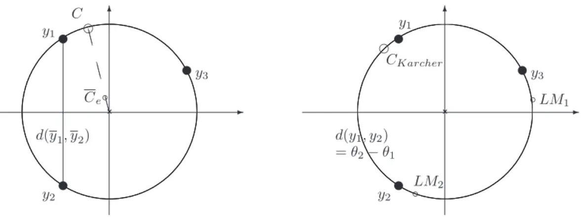
The main advantage of Definition 1 is that the IAM and AIAM are easily computed, in contrast to the Karcher mean. The latter gets even more problematic to evaluate as soon as the agents are not located in a convex set of G, which causes no difficulty for the IAM; as an illustration, see the local minima LM1 and LM2appearing in the computation of the Karcher mean on Figure 1,
while the IAM is directly found thanks to the following property.
The IAM and AIAM are closely related to the well-known notion of centroid in E.
Definition 2: The (weighted) centroid Cein E of N agents located at y1...yN in G ⊂ E is defined
as Ce= 1 W N X k=1 wkyk, W = N X k=1 wk. (11)
Since the norm kck2 is constant, by considering the y
k as m-vectors, one easily verifies that
alternative definitions for the IAM and AIAM are
C = argmax c∈G (cTC e) and AC = argmax c∈G (−cTC e) . (12)
Hence, the computation of the IAM and AIAM just involves the search for the global maxima of a linear function on E in a very regular search space (namely, a CC Lie group).
Local maximization methods even suffice provided that the linear function has no maxima on
G other than the global maxima. It turns out that this is the case for many Lie groups and
homo-geneous manifolds, including SO(n) and Grass(p, n) with the embeddings of the present paper, as well as the canonically embedded n-dimensional sphere in Rn+1. In absence of a formal proof
in the literature, the following blanket assumption is formulated; it must be seen as a condition on the Lie group, maybe including the way it is embedded, which is emphasized with the notation
G.
Assumption 1: The local maxima of a linear function f (c) = cTb over c ∈ G, with b fixed in E,
3.1.2 Examples
The circle: The canonical embedding of SO(2) ∼= S1in R2satisfies Assumption 1. C
eis simply
the average of the corresponding positions in R2 and C is its central projection onto the circle.
Hence C corresponds to the whole circle when Ce = 0 (i.e. the centroid in R2 is located at the
center of the circle) and reduces to a single point in other situations; using a polar representation of Ce∈ R2∼= C, this writes C = ½ arg(Ce) , Ce6= 0 S1, C e= 0 .
The Karcher mean may also contain multiple points when Ce= 0 (for example, when all the agents
are uniformly distributed around the circle), but generally not the whole circle. The Karcher mean uses the arc length between two points as their distance, while the IAM considers the “chordal” distance in R2. The difference between IAM and Karcher mean is illustrated on Figure 1.
-6 u y1 u y2 uy3 d(y1, y2) b CC CC CC Ce e C -6 u y1 u y2 uy3 d(y1, y2) = θ2− θ1 e CKarcher b LM1 b LM2
Figure 1: Induced arithmetic mean C and Karcher mean CKarcher of 3 equally-weighted points on the circle. In addition to the different positions of the two means, note the local minima LM1
and LM2appearing in the computation of the Karcher mean.
The special orthogonal group: SO(n) is embedded in Rn×n with the usual matrix
represen-tation. The group SO(n) acts by matrix multiplication on Rn×n and the Frobenius norm of an
orthonormal matrix is kQkk =
p
trace(QTQ) =ptrace(In) =√n.
On SO(n), Ce=
P
kQk is a general n × n matrix. The induced arithmetic mean is linked to
the polar decomposition of Ce: any square matrix B can be decomposed into a product U R where
U is orthogonal and R is symmetric positive semi-definite; R is always unique, U is unique if B is
non-singular [72]. The matrix U obtained is the point in O(n) that is closest to B according to the canonical distance of Rn×n. As a consequence, when det(C
e) ≥ 0, the induced arithmetic mean
contains the matrices U with positive determinant obtained from the polar decomposition of Ce;
this fact has already been noticed and proven in [46]. When det(Ce) ≤ 0, the result is somewhat
more complicated but also has a closed-form solution.
Proposition 1: The induced arithmetic mean C of N points on SO(n) is characterized as follows.
• If det(Ce) ≥ 0, C contains the matrices U with positive determinant resulting from the
polar decomposition U R of Ce; it reduces to a single point when the multiplicity of 0 as an
• If det(Ce) ≤ 0, C = U HJHT where U is an orthogonal matrix of negative determinant
re-sulting from the polar decomposition U R of Ce, H contains the orthonormalized eigenvectors
of R with an eigenvector corresponding to the smallest eigenvalue of R in the first column, and J = µ −1 0 0 In−1 ¶ .
Now C reduces to a single point when the smallest eigenvalue of R has multiplicity 1.
Proof: The proof is postponed because it makes use of calculations presented later in the section. Specifically, it will first be shown that SO(n) satisfies Assumption 1. Then the analytical form of the IAM is established by selecting the local maxima among the critical points of (12).
4
These examples exclusively considered the induced arithmetic mean; note that from (12), the conclusions are trivially modified for the anti-[induced arithmetic mean] by replacing Cewith −Ce.
3.2
Consensus as an optimization task
3.2.1 Definition
Consider a set of N agents on a CC Lie group satisfying Assumption 1 and denote their embedded positions by yk. Suppose that the agents are interconnected according to a fixed digraph G of adjacency matrix A = [ajk]. In the remainder of this report equal weights wk = 1 are assigned
to all agents for notational convenience; the generalization to weighted agents is straightforward. The following definitions are introduced in the present work.
Definition 3: N agents are said to have reached synchronization when they are all located at
the same position on G.
Definition 4: N agents are said to have reached a consensus configuration with
communica-tion graph G if each agent k is located at a point of the induced arithmetic mean of its neighbors j à k, weighted according to the strength of the communication links:
yk ∈ argmax c∈G cT N X j=1 ajkyj ∀k . (13)
Similarly, N agents are said to have reached an anti-consensus configuration when the previous definition is satisfied by replacing the IAM by the AIAM:
yk∈ argmin c∈G cT N X j=1 ajkyj ∀k . (14)
The consensus defined by (13-14) is graph-dependent; this can be interpreted as the fact that each agent considers that it has reached consensus when it is located at the best possible place according to the agents from which it receives information. In the case of a tree or an equally-weighted complete graph Gc, consensus means synchronization.
Proposition 2: When G is a tree or G = Gc, the only possible consensus configuration is
Proof: For the complete graph, according to Definition 4, at consensus the property yT k X j6=k yj≥ cT X j6=k yj
must be satsified for all k and any c ∈ G. Furthermore, it is obvious that yT
kyk > yTkc for any c 6= yk ∈ G. As a consequence, at consensus yT k N X j=1 yj> cT N X j=1 yj
for any c 6= yk ∈ G. According to (12), this means that yk is located at the IAM of all the agents
(including itself), and moreover that the latter reduces to a single point. Since this must hold for all k, all the agents must be located at this single point (which is then trivially their IAM).
For the tree, start with all agents fixed except a leaf k. The obvious unique IAM of the neighbors of k is the position of its parent; therefore all leaves must be synchronized with their parent. Now consider synchronized moves of a parent j and its leaves. As the leaves follow j everywhere, the obvious global minimum in (7) occurs when j is synchronized with its own parent, which brings us back to the previous situation. An inductive argument is then used up to the root.
4
Synchronization is a configuration of complete consensus. It is the only consensus configuration common to all graphs. The opposite of synchronization is more difficult to define because there exists no anti-consensus configuration common to all graphs. A meaningful property to charac-terize a configuration of complete anti-consensus would be to require that the IAM of the agents is the entire manifold G. This is called a balanced configuration in the present work.
Definition 5: N agents are said to be in a balanced configuration when their induced arithmetic
mean is the entire manifold G.
Balancing implies some spreading of the agents on the manifold. It can be a meaningful objec-tive in several applications. Nevertheless, a full characterization of balanced configurations seems complicated. Balanced configurations do not always exist (typically, when the number of agents is too small relative to the manifold dimension) and are mostly not unique (they can appear in qualitatively different forms). Finally, the following link exists between anti-consensus for Gcand
balancing.
Proposition 3: All balanced configurations are anti-consensus configurations for Gc.
Proof: Note that for the equally-weighted complete graph, (14) can be written as
yk∈ argmin c∈G ¡ cT(N C e− yk) ¢ ∀k . (15)
Assume that the agents are in a balanced configuration. This means that f (c) = cTC
e must be
constant over c ∈ G. Therefore condition (15) reduces to yk = yk which is trivially satisfied.
4
Note that in contrast to Proposition 2, Proposition 3 does not establish a necessary and sufficient condition: anti-consensus configurations for Gc that are not balanced do exist, though
3.2.2 Examples
The circle: In [13] and [14], (anti-)consensus configurations are fully characterized for an equally-weighted complete graph on the circle S1 ∼= SO(2). It is shown that (for N > 1) the only
anti-consensus configurations that are not balanced occur for N odd and correspond to (N +1)/2 agents at one position and (N − 1)/2 agents at the opposite position on the circle. It is not difficult to show that balanced configurations are unique for N = 2 and N = 3, while there is a continuum of such configurations for N > 3.
Another situation where (anti-)consensus configurations are not too difficult to characterize is for the equally-weighted undirected ring interconnection graph in which each agent k is connected to two neighbors such that the graph forms a single closed undirected path. In this case, regular configurations are states where consecutive agents in the path are all separated by the same angle χ ≥ 0; it turns out that χ ≤ π/2 corresponds to consensus configurations and that χ ≥ π/2 corresponds to anti-consensus configurations. In addition, for N ≥ 4, there are irregular consensus and anti-consensus configurations where non-consecutive angles of the regular configurations are replaced by (π − χ/2). As a consequence:
• There are several possible qualitatively different consensus and anti-consensus configurations.
• There are consensus and anti-consensus states which correspond to equivalent configurations when discarding the underlying graph. For example, the positions occupied by the agents are strictly equivalent for 7 agents separated by 2π/7 (consensus) or separated by 4π/7 (anti-consensus); the only difference, based on which agent is located at which position, concerns the way the communication links are drawn.
• There may even be degenerate configurations that correspond to consensus and anti-consensus (for example when consecutive agents are separated by π/2 for N = 4, 8, ...); this singularity is specific to the undirected ring graph.
• There is no common anti-consensus state for all possible ring graphs. Indeed, considering an agent k, a common anti-consensus state would require that for any two other points selected as neighbors of k, either they are separated by π or they are at both sides of k at a distance
χ ≥ π/2; one easily verifies that this cannot be satisfied for all k.
The special orthogonal group: Simulations of the algorithms proposed in this paper suggest that balanced configurations always exist for N ≥ 2 when n is even and for N ≥ 4 when n is odd. Furthermore, convergence to an anti-consensus state for Gcthat is not balanced is never observed.
3.2.3 Consensus optimization strategy
The presence of a maximization condition in the definitions of the previous sections naturally points to the use of optimization methods to compute (anti-)consensus configurations. As a consequence, it is natural to introduce a cost function whose optimization leads to (anti-)consensus configurations.
For a given graph G with adjacency matrix A = [ajk] and associated Laplacian L(i) = [l(i)jk],
the cost function PL is defined as
PL(y) = 1 2N2 N X k=1 N X j=1 ajkyTjyk= cst1− 1 4N2 N X k=1 N X j=1 ajkkyj− ykk2 (16)