A study on trade-offs between spatial resolution and temporal sampling density for wheat yield estimation using both thermal and calendar time

(1)

Contents lists available atScienceDirect

Int J Appl Earth Obs Geoinformation

journal homepage:www.elsevier.com/locate/jag

A study on trade-o

ﬀs between spatial resolution and temporal sampling

density for wheat yield estimation using both thermal and calendar time

Yetkin Özüm Durgun

a,b,

*, Anne Gobin

b,c

, Grégory Duveiller

d

, Bernard Tychon

a

a_{Département Sciences et Gestion de l’Environnement, Université de Liège, Avenue de Longwy 185, 6700 Arlon, Belgium} b_{Vlaamse Instelling voor Technologisch Onderzoek (VITO), Boeretang 200, B-2400 Mol, Belgium}

c_{Faculty of BioScience Engineering, Department of Earth & Environmental Sciences, University of Leuven, Celestijnenlaan 200E, B-3001 Leuven, Belgium} d_{European Commission, Joint Research Centre (JRC), Via E. Fermi 2749, I-21027 Ispra, Italy}

A R T I C L E I N F O Keywords: Yield estimation Thermal time Winter wheat NDVI PROBA-V Northern France A B S T R A C T

Within-season forecasting of crop yields is of great economic, geo-strategic and humanitarian interest. Satellite Earth Observation now constitutes a valuable and innovative way to provide spatio-temporal information to assist such yield forecasts. This study explores different configurations of remote sensing time series to estimate of winter wheat yield using either spatiallyfiner but temporally sparser time series (5daily at 100 m spatial resolution) or spatially coarser but denser (300 m and 1 km at daily frequency) time series. Furthermore, we hypothesised that better yield estimations could be made using thermal time, which is closer to the crop phy-siological development. Time series of NDVI from the PROBA-V instrument, which has delivered images at a spatial resolution of 100 m, 300 m and 1 km since 2013, were extracted for 39fields for field and 56 fields for regional level analysis across Northern France during the growing season 2014-2015. An asymmetric double sigmoid model wasfitted on the NDVI series of the central pixel of the field. The fitted model was subsequently integrated either over thermal time or over calendar time, using different baseline NDVI thresholds to mark the start and end of the cropping season. These integrated values were used as a predictor for yield using a simple linear regression and yield observations atfield level. The dependency of this relationship on the spatial pixel purity was analysed for the 100 m, 300 m and 1 km spatial resolution. Atfield level, depending on the spatial resolution and the NDVI threshold, the adjusted R² ranged from 0.20 to 0.74; jackknifed– leave-one-field-out cross validation– RMSE ranged from 0.6 to 1.07 t/ha and MAE ranged between 0.46 and 0.90 t/ha for thermal time analysis. The best results for yield estimation (adjusted R² = 0.74, RMSE =0.6 t/ha and MAE =0.46 t/ha) were obtained from the integration over thermal time of 100 m pixel resolution using a baseline NDVI threshold of 0.2 and without any selection based on pixel purity. Thefield scale yield estimation was aggregated to the regional scale using 56fields. At the regional level, there was a difference of 0.0012 t/ha between thermal and calendar time for average yield estimations. The standard error of mean results showed that the error was larger for a higher spatial resolution with no pixel purity and smaller when purity increased. These results suggest that, for winter wheat, afiner spatial resolution rather than a higher revisit frequency and an increasing pixel purity enable more accurate yield estimations when integrated over thermal time at thefield scale and at the regional scale only if higher pixel purity levels are considered. This method can be extended to larger regions, other crops, and other regions in the world, although site and crop-specific adjustments will have to include other threshold temperatures to reflect the boundaries of phenological activity. In general, however, this methodological ap-proach should be applicable to yield estimation at the parcel and regional scales across the world.

1. Introduction

Accurate and timely yield estimates are important due to their large impact on strategic planning and world markets (Doraiswamy et al., 2007). Extensive research has been done over the past decades to apply

remote sensing for predicting yields at different scales, from field to national levels. Therefore, these studies are crucial for individual farmers, national governments and international organizations. Sa-tellite images have different spectral, temporal and spatial resolutions. The images most commonly used for regional studies of yield

https://doi.org/10.1016/j.jag.2019.101988

Received 24 June 2019; Received in revised form 2 October 2019; Accepted 3 October 2019

⁎_{Corresponding author. Present address: Research Institutes of Sweden (RISE), Sven Hultins plats 5, vån 4, 412 58 Göteborg, Sweden.} E-mail addresses:ozum.durgun@ri.se(Y.Ö. Durgun),anne.gobin@vito.be(A. Gobin),gregory.duveiller@ec.europa.eu(G. Duveiller), bernard.tychon@ulg.ac.be(B. Tychon).

T

(2)

estimation still have a coarse resolution and a daily revisit time. Time-series data from the Advanced Very High Resolution Radiometer (AVHRR), Satellites Pour l’Observation de la Terre or Earth-observing Satellites VeGeTation (SPOT-VGT), MODerate resolution Imaging Spectroradiometer (MODIS), and MEdium Resolution Imaging Spec-trometer (MERIS) are examples of low-resolution data. Low-resolution images have been used to establish statistical regressions between Ve-getation Indices (VIs) and crop yield statistics (Doraiswamy et al., 2007; Duncan et al., 2015). The main advantage of coarse spatial resolution data for statistical prediction of yield is their longer historical time series, often crucial to relate present conditions to similar conditions observed in the past. Other advantages of coarse spatial resolution data is their associated high temporal resolution, low cost, and global cov-erage which allows following vegetation development even when overcast conditions frequently occur (Atzberger, 2013; Junior et al., 2014;Kibet, 2016;Rembold et al., 2013).

Despite their valuable input for assessing crop production, the most relevant limitation of coarse spatial resolution time-series data is that their spectral reflectances contain mixed information from several surfaces and vegetation types, making it difficult to interpret the signal and directly relate a spectral or temporal signature to a specific crop condition (Kibet, 2016). This problem should gradually disappear with the establishment of time series of images with higher spatial resolu-tions, such as the combination of Landsat-8 with Sentinel-2 (Claverie et al., 2018). However, this also comes with additional constraints of having to deal with much more data volume and thus processing time. A middle ground may be data from the Project for On-Board Autonomy-Vegetation (PROBA-V) satellite, which delivers data at 100 m every 5 days. The advantage of the 100 m dataset compared to higher spatial resolution satellite data is that its spatio-temporal resolution is suffi-cient for yield estimate studies, thereby avoiding larger processing times of heavier data volumes (Duveiller and Defourny, 2010). The PROBA-V time series became available in May 2013, and, as a result, few studies exist that relate PROBAV data to crop yield (Meroni et al., 2016;Zheng et al., 2016). The specific comparison of PROBAV data at different resolutions – 100 m, 300 m and 1 km – for crop yield estima-tion has not been studied to date.

From satellite observations, the vegetation signal can be captured through mathematical combinations of reflectances from different spectral bands into what are known as vegetation indices (VIs), such as the Normalized Difference Vegetation Index (NDVI) (Rouse et al., 1974). Several studies have demonstrated that seasonal VIs are sig-nificantly correlated with official crop yield statistics (Bégué et al., 2010; Doraiswamy et al., 2007; Ferencz et al., 2004; Meroni et al., 2013; Pinter et al., 1981; Rasmussen, 1992). Consequently, remote sensing is an attractive tool for monitoring spatio-temporal patterns of vegetation growth (Duncan et al., 2015). Measures of green vegetation provided by VIs can be used to estimate yield. Using SPOT-VGT imagery at 1 km,Meroni et al. (2013)computed the integral between the start of the growing season and the beginning of the descending stage for winter wheat yield estimates at a national level and discovered a sig-nificant correlation.

Vegetation indices can be expressed as a function of thermal time instead of calendar time to derive more crop physiologically sound relations. Characterising crop physiological development in relation to thermal time is a modelling approach that has been used in weather and climate impact research (Gobin, 2012, 2018). Plants require certain accumulated heat energy over the growing season to develop. Thermal time for organ growth and development depends on the temperature (Duveiller et al., 2013;Meroni et al., 2013) and can be deﬁned as the cumulative daily average temperature throughout the growing period, expressed as the Growing Degree Day (GDD) (Franch et al., 2015; Gobin, 2010;Kouadio et al., 2012). The GDD has been used to obtain smoother and more temporally consistent time series of biophysical variables (Duveiller et al., 2013).Lobell et al. (2003)have used GDD rather than calendar days to account for changes in crop development

due to accumulated temperature.Skakun et al. (2017)have used GDD to account for discrepancies which are temporally and spatially non-uniformities of the winter crop development due to the presence of diﬀerent agro-climatic zones.

Pixel purity represents the relative contribution of the surface of interest to the signal detected by the remote sensing instrument (Duveiller, 2012). This approach has been used to restrict the analysis to a subset of a region’s pixels and to identify meaningful samples for both crop growth monitoring (Durgun et al., 2016a; Duveiller and Defourny, 2010) and crop area estimation (Durgun et al., 2016b;Löw and Duveiller, 2014). Several studies have demonstrated that a better characterization of crop growth can be obtained by focusing on subset of pixels that are dominated by a larger proportion of crop area (Chen et al., 2016;Huang et al., 2016;Kastens et al., 2005;Löw and Duveiller, 2014; Waldner et al., 2016). For the present study, the degree of homogeneity of the signal with respect to the target crop is here deﬁned as pixel purity; and it allows explicit control over the relationship be-tween the remote sensing observation and the target.

Satellite remote sensing observations of greenness using indices such as NDVI have proven useful for within season crop forecasting but establishing adequate time series of such information requires a trade-off between: (1) how fine the spatial resolution must be; (2) how fre-quently a field needs to be revisited; and (3) how long the corre-sponding archive needs to be (Houborg and McCabe, 2018;Tian et al., 2013). Whilst new technology is guaranteeing improvements in thefirst two points with new constellations such as Sentinel-2 (10 m, 5-day re-visit, since 2015), the third point typically remains a limitation for crop monitoring, advocating further research on EO-data series. With its central camera, PROBA-V provides an opportunity to estimate yield at 100 m resolution, but this still comes at the expense of a lower revisit frequency. Both spatial resolution and temporal resolution of the data obtained from satellite products could affect the accuracy of crop yield estimates. Therefore, depending on what the end-user wants, there can be a trade-off between spatial and temporal resolution in terms of minimum information required to obtain good results. The main ob-jective of this study is to investigate whether it is better to use 100 m dataset with more data in space, but less in time, or it is better to use 300 m (and 1 km) dataset(s) with less data in space and more in time.

2. Materials

2.1. Study area and ground data

The study area encompassed Nord-Pas-de Calais, Picardie and Champagne-Ardenne in Northern France (Fig. 1). These regions are amongst the highest wheat-producing regions of France.

Ground data,field boundaries and winter wheat yields were ob-tained from farmers’ declarations during the 2015 crop campaign by a private company called Drone Agricole. Yield values in the ground data were measured by weighing harvest instead of guessing. The sowing dates were in October and November and the harvest took place in July and August. After applyingfield selection thresholds further explained in the Methods section, 39 winter wheatfields from a total of 56 fields were selected with sizes ranging from 8 ha to 12.5 ha. Average yield for the area was around 10 t/ha with a standard deviation of 1.2 t/ha. Neighbouringfields can have different yields which can be explained by different biophysical environments such as soil type, and by different management strategies relating to cultivar, sowing time, and agri-che-mical application rates.

2.2. NDVI and meteorological data

PROBA-V was launched in May 2013 toﬁll the gap between the SPOT-VGT and Sentinel-3 satellites. PROBAV has four spectral bands: blue, centred at 0.463μm; red at 0.655 μm; NIR at 0.845 μm; and SWIR at 1.600μm. The instrument has a swath width of 2250 km across four

(3)

bands. The central camera of the PROBA-V satellite provides a global coverage at a 5-daily 100 m resolution, whereas global daily images are acquired at 300 m and 1 km resolutions. Daily atmospherically cor-rected PROBA-V NDVI images and status maps at 100 m, 300 m and 1 km resolutions were obtained fromhttp://www.vito-eodata.be. Status maps, containing information about snow, ice, shadow, clouds and land or sea for every pixel, were used to extract high quality pixels and NDVI series.

Meteorological input, daily minimum and maximum temperatures, were available at a 0.25 × 0.25 ° grid from the Joint Research Centre Monitoring Agriculture by Remote Sensing OPerational (JRC-MARSOP) project (Baruth et al., 2007). The MARSOP meteorological data are collected from ground stations in near real time for diﬀerent hours within one day and provided directly by national meteorological in-stitutes or regional authorities.

3. Methods

NDVI values at 100 m, 300 m and 1 km resolutions were extracted for the central pixel of eachfield where yield data were available. The number of NDVI observations during the growing season can severely affect the integral calculated after curve fitting. Because of its lower revisit time, the 100 m dataset resulted in a temporally sparser time series compared to the 300 m and 1 km resolution datasets. Twofield selection thresholds were therefore applied to retain thefields for which sufficient data were available for the three datasets. The selection cri-teria were: (1) a minimum of 10 cloud-free NDVI observations from PROBA-V during the growing season and (2) less than two-month gaps between two consecutive observations. Based on these criteria, only 39 winter wheatfields out of 56 fields were retained for the 100 m data, while all 56 where kept for the 300 m and 1 km datasets.

Pixel purity percentages were investigated for the three resolution

datasets to study the effects. The same purity thresholds were defined for all datasets, although the differences between the resolutions and associated sample sizes were present. For instance, for the 1 km dataset, the number of pixels within thefields was too low for a 20 % purity threshold, whereas for the 100 m dataset, almost all the pixels had more than 95 % purity.

Temperature values were extracted from the JRC-MARSOP database (Baruth et al., 2007), and thermal time was computed in cumulative GDD (Eq. 1). = + − GDD T T T 2 max min base ₍₁₎

where Tmaxis the maximum daily temperature, Tminis the minimum daily temperature and Tbase is the base temperature. The base tem-perature for wheat was 0 °C, as used byDuveiller et al. (2012). Allﬁelds in the study site belonged to the same climatic region. The period used for the calculation of the cumulative GDD was from the beginning of January until the end of July.

Remotely sensed imagery time series are irregular due to cloud contamination, and therefore relationships are sought to estimate growth development during the season. An asymmetric double sigmoid function (ADSF) wasfitted to the NDVI time series of the central pixel of eachfield for thermal time and for calendar time. The ADSF is a variant of the canopy structure dynamic model curves proposed byKoetz et al. (2005). As applied byZhong et al. (2014), the ADSF was used for curve fitting and expressed as follows in (Eq. 2):

= + − − −

V t( ) V 1V tanh p t D tanh q t D

2 [ ( ( )) ( ( ))]

b a i d ₍₂₎

where V(t) is the NDVI at the time t. Vbis the background NDVI value corresponding to the non-growing season. Vais the amplitude of NDVI variation within the current growing cycle. The overall changing rates of the slopes were characterized by p and q. Middle dates of the Fig. 1. Location of winter wheatﬁelds, yields (t/ha) and soil type of the study area.

(4)

increasing and the decreasing segments were represented by Diand Dd. A cumulated NDVI value is calculated for allfitted curves for each field at each of the 100 m, 300 m and 1 km spatial resolutions, each time using a different NDVI baseline value ranging from 0 to 0.6. A linear regression was calculated between yield data and the integral values of thefitted ADSF for each field. The statistical metrics, namely the adjusted coefficient of determination (R²), Pearson’s correlation’s (r) associated p-value, jackknifed (leave-one-field-out cross validation) RMSE (t/ha) and MAE (t/ha), were used to evaluate the goodness offit. Finally, to provide an idea of how these estimates can represent a regional yield, the average of all the estimated yields for all points at 100 m, 300 m and 1 km was calculated and compared with the average observed yield of all 56 fields. Additionally, the percentage change between the average of the estimated and observed yield, and the standard error of mean (SE) were calculated. The calculation was done by using an NDVI threshold of 0.2 and for all pixel purity percentages.

4. Results

Thefitted ADSF integral areas demonstrated a higher goodness of fit with an increase in pixel purity and resolution of the PROBA-V NDVI datasets at 100 m, 300 m and 1 km resolutions for thermal time and calendar time as shown for one field with a 0.3 NDVI threshold in Fig. 2.

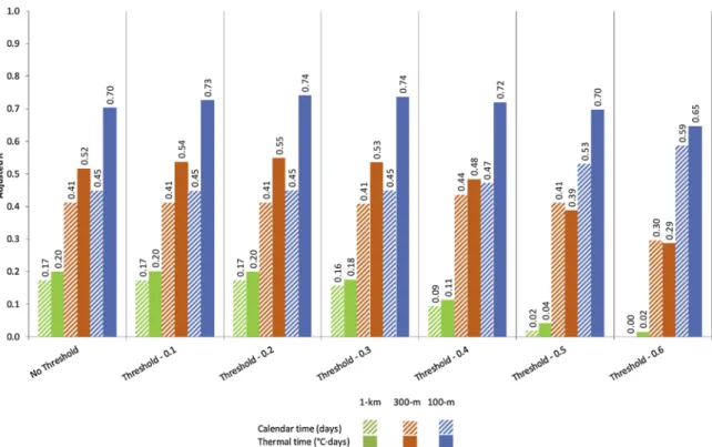
Fig. 3summarizes the performance across all sampledfields for the different spatial resolutions, baseline NDVI thresholds, and for thermal versus calendar time integration. The results illustrate that the 100 m dataset performed better than the 300 m NDVI which, in turn, per-formed better than the 1 km for both the thermal time and calendar time analyses. This demonstrates that afiner spatial resolution ensured a purer crop signal and better yield estimation at thefield level, pre-sumably as it contained less contamination from adjacent land cover. The integrations on the over thermal time performed almost system-atically better that those based on calendar time, with the marginal exceptions at 300 m resolution with high baseline NDVI thresholds of 0.5 and 0.6. Compared to calendar time, integration over thermal time Fig. 2. Example of NDVI time series extracted for a singlefield located in Nord-Pas-de Calais (50.879 °N, 2.218 °E) at various spatial resolutions. The left column shows time series in normal calendar time (in days) from pixel sizes of (a) 100 m, (c) 300 m and (e) 1 km; while the right column shows the same series respectively in (b), (d) and (f) in thermal time (°C·days). The grey line represents thefitted ADSF curve, and the shaded area represents the integral above a given NDVI threshold (in this case equal to 0.3). Note that in this example different minimum tolerable pixel purity thresholds have been used for different scales.

(5)

showed a better performance by 15 % for 1 km, 33 % for 300 m, and 65 % for 100 m for an NDVI threshold of 0.2 in adjusted R² (Fig. 3). The optimal baseline NDVI threshold appeared to be between 0.2 and 0.3, while higher thresholds reduced the performance.

The results are presented against both the actual yield and the in-tegral values at 100 m, 300 m and 1 km resolutions for NDVI threshold 0.2 in the scatterplots inFig. 4. There were noticeable diﬀerences be-tween the three resolution results. In addition, deviation from the 1:1 line was less pronounced for thermal time as compared to calendar time. The relation between actual yield and integral values was stronger for at 100 m resolution compared to at 300 m and 1 km resolutions.

The relationships between yield and the integrated NDVI based on ADSF were statistically signiﬁcant. In all cases, p-values were smaller than 0.001, except for the p-values for NDVI thresholds of 0.5 and 0.6 at the 1 km resolution, which were larger than 0.05 (Fig. 5). Integration over thermal time with a 0.2 NDVI threshold gave the strongest results at the 100 m, 300 m and 1 km resolutions. The best result was obtained at 100 m resolution with MAE and RMSE for NDVI threshold 0.2 for thermal time equalling to 0.46 and 0.60 t/ha respectively.

The pixel-crop coverage in terms of amount of the cropfield covered by the pixel also influenced the results. The effect of selecting pixels with increasingly higher crop specific purity is reported in Table 1. Naturally, pixel purity percentages increased withfiner spatial resolu-tion. The pixel purity percentages encountered in the dataset ranged between 61 %–100 % for the 100 m time series, between 14 %–100 % for the 300 m time series and between 2 %–51 % for the 1 km time series. The same purity thresholds were used for pixel purity compar-isons of calendar time (days) and thermal time (°C·days) at 100 m, 300 m and 1 km resolutions for different NDVI thresholds (Table 1).

The adjusted R² values (Table 1) illustrate how correlation between the integrated NDVI and yield increases with higher pixel purities. These results demonstrated that high quality yield estimates were possible at lower resolutions when a higher pixel purity was imposed. However, more stringent pixel purity percentages come at the expense of the number offields that can be analysed, which potentially can jeopardize the capacity of the sample set to represent the regional yield. This analysis involving purity thresholds generally confirms that thermal time outperformed calendar time, but a notable exception Fig. 3. Mean adjusted R² comparison of calendar (days) and thermal time (°C·days) at 100 m, 300 m and 1 km resolutions for different NDVI thresholds applied at all fields without purity threshold. The number of the fields used is the same.

Fig. 4. Scatterplots comparing the actual yield with integral values at 100 m, 300 m and 1 km resolutions for NDVI threshold 0.2. TT is thermal time and CT is calendar time.

(6)

Fig. 5. Jackknifed RMSE (t/ha) and MAE (t/ha) for calendar (in days) and thermal time (in °C·days) analyses at 100 m, 300 m and 1 km resolutions withoutﬁltering by pixel purity and for diﬀerent NDVI thresholds. p-values are smaller than 0.001 in all cases, except for the ones labelled with a star symbol, which were larger than 0.05.

(7)

occurred for samples with purity above 65 % for calendar time at 300 m. In this speciﬁc situation, the R² increased substantially for ca-lendar time. However, the sample size became small (12 and 5 from a total of 39) and may not be representative of the general situation.

Fig. 6 presents the average estimated yield (t/ha) difference be-tween spatial resolution datasets, which was relatively small. The ca-lendar time performed nearly the same as the thermal time. Overall, the standard error of mean results showed that lower spatial resolution data performed better when purity was decreasing, and higher spatial re-solution data performed better when purity was rising.Fig. 6shows that when taking allfields together, the 100 m fields suffered from a mar-ginal penalty due to a more limited number of samples than 300 m data (39 vs 56). However, as the subset offields for the 300 m (and 1 km) data diminished due to increasing purity thresholds, and increasing bias against the average regional yield was observed, while the 100 m data remained very stable.

5. Discussion

This study shows that thefitted ADSF integral area of NDVI values using thermal time provided a better estimation for yield at thefield scale than using the conventional calendar time. As long as this in-tegration was done using a low NDVI baseline (e.g. NDVI = 0.2), this finding held true for all three pixel sizes (100 m, 300 m and 1 km), al-though the improvement was much larger for thefiner spatial resolu-tion. This suggests that for the landscape observed here, there is a considerable added-value in favouring a finer spatial resolution as it enables a diagnostic that adheres closer to the dynamics of the crop field due to reduced noise from neighbouring landscape elements. This result could be extended to any other landscape with similarfield sizes and geometries. However, a more general outcome that should be ap-plicable to even more varied types of landscapes is that for all spatial resolutions, the time representation based on thermal time was more appropriate and resulted in a higher explanatory power of yield esti-mation, presumably due to a closer representation of crop physiology. Importantly, the predictive power atfield scale was high for the finer pixel size despite the considerably lower revisit frequency of the PROBA-V 100 m instrument, i.e. 5-daily, which is caused by the smaller swath of the central camera. The double-sigmoid model effectively re-sembled a semi-empirical crop growth model that relied on a few data points as long as thermal time was used. In fact,Fig. 3 and 5show that for all the fields, except for those with very high NDVI baseline in-tegration thresholds, the denser 100 m time series integrated over thermal time performed better than the 300 m time series integrated over calendar time. Thermal time integration of the double-sigmoid model outperformed calendar time integration.

Although the 100 m pixel time series showed a clear advantage when used with thermal time smoothing, the total number of time series that could be used in this study was reduced because several fields had too few valid observations due to cloud cover. Therefore, 17 fields had to be discarded for further field scale yield estimation. This restriction can be a disadvantage when the interest is the regional yield forecast based on a representative sample offields rather than the yield

of individualfields. However, for the particular case of this study area, our results showed that at the regional level, the average yield esti-mation difference was relatively small (0.0012 t/ha) between different spatial resolutions both for calendar and thermal time. The difference was larger with an increase in pixel purity thresholds, as this resulted in a more restrictive sample set that, in this specific case, appeared to be different from the regional mean. As a consequence, the standard errors of the mean are lower for the lower spatial resolution. However, this is not a general conclusion that can be extended to other situations in which, for example, largerfields may not be so representative of the regional mean.

This study has further contributed in demonstrating the potential of using satellites with the configuration of PROBA-V to assess winter wheat yield. Since PROBA-V is a relatively new satellite, there are limited studies available for crop yield estimation. This study’s results aligned with reported ranges (Meroni et al., 2016;Zheng et al., 2016). Zheng et al. (2016)generated 100 m land surface reflectances by fusing the PROBA-V 100 m and 300 m S1 products, and achieved 0.663 for R², 0.63 for RMSE (t/ha) and 7.27 % for RRMSE at Yucheng County, and 0.631 for R², 0.42 for RMSE (t/ha) and 4.88 % for RRMSE at Guantao County for winter wheat yield estimates in China for one growing season in 2014–2015 (Zheng et al., 2016). In another study, Meroni et al. (2016)evaluated the NDVI data continuity between SPOT-VGT and PROBA-V missions for operational yield forecasting in North African countries for yield estimates of barley, soft wheat and durum wheat. They obtained 0.78 for R² and 4.51 for RMSE difference in percentage in Morocco, 0.94 for R² and 3.27 for RMSE difference in percentage in Algeria, and 0.91 for R² and -31.76 for RMSE difference in percentage in Tunisia. In the present study, the adjusted coefficients of determination (R²) were 0.2 at 1 km, 0.55 at 300 m, and 0.74 at 100 m resolutions. The jack-knifed RMSE amounted to 1.07 t/ha for 1 km resolution, 0.79 t/ha for 300 m resolution and 0.60 t/ha for 100 m resolution, while MAE was 0.78 t/ha for 1 km resolution, 0.53 t/ha for 300 m and 0.46 t/ha for 100 m resolutions. For all three resolution datasets, it was overestimated in the low yield value and under-estimated in the high yield values. Such a bias was not uncommon in regression models.

The results of our study closely agree with other studies that com-pared the performance of the spatial resolutions of satellites. Guindin-Garcia evaluated MODIS 8-day and 16-day composite products for monitoring maize yield using the green leaf area index (LAIg) ( Guindin-Garcia, 2010). The results revealed that 250 m MODIS products pro-vided more accurate estimates of maize LAIgcompared to 500 m pro-ducts during the entire growing season (Guindin-Garcia, 2010).Chen et al. (2006)assessed the potential use of the MODIS Enhanced Vege-tation Index (EVI) at 250 m, 500 m and 1 km resolutions for monitoring maize. According to their results, MODIS EVI at 1 km data had lower EVI values compared to 250 m and 500 m data in the vegetative stage. The reason was that the higher resolution pixels contained a larger proportion of agricultural coverage (Chen et al., 2006). The particu-larity of this present study compared to the mentioned studies is that this study investigated the impact of low revisit time of 100 m resolu-tion dataset and high revisit time of 300 m and 1 km datasets. Table 1

Adjusted R² results for minimum pixel purity comparison for calendar time (days) and thermal time (°C·days) analyses at 100 m, 300 m and 1 km resolutions for diﬀerent NDVI thresholds (ranging from 0 to 0.3) and pixel purity thresholds (ranging from 0 to 90 % or more). The colour code should be read for the whole table ranging from red (low values), yellow (mid- values) to green (high values). (For interpretation of the references to colour in this Table legend, the reader is referred to the web version of this article).

0 15 40 65 90 0 15 40 65 90 0 15 40 65 90 0 15 40 65 90 0 15 40 65 90 0 15 40 65 90 39 39 39 37 34 39 39 39 37 34 39 37 27 12 5 39 37 27 12 5 39 9 1 0 0 39 9 1 0 0 No 0.4 0.4 0.4 0.5 0.6 0.7 0.7 0.7 0.7 0.7 0.4 0.4 0.5 0.8 0.9 0.5 0.5 0.6 0.6 0.6 0.2 0.3N/A N/A N/A0.2 0.3 N/A N/A N/A 0.1 0.4 0.4 0.4 0.5 0.6 0.7 0.7 0.7 0.7 0.8 0.4 0.4 0.5 0.8 0.9 0.5 0.5 0.6 0.6 0.6 0.2 0.3N/A N/A N/A0.2 0.4 N/A N/A N/A 0.2 0.4 0.4 0.4 0.5 0.5 0.7 0.7 0.7 0.7 0.8 0.4 0.4 0.5 0.8 0.9 0.5 0.5 0.6 0.7 0.7 0.2 0.3N/A N/A N/A0.2 0.4 N/A N/A N/A 0.3 0.4 0.4 0.4 0.5 0.5 0.7 0.7 0.7 0.7 0.8 0.4 0.4 0.5 0.8 0.9 0.5 0.5 0.6 0.6 0.6 0.2 0.2N/A N/A N/A0.2 0.3 N/A N/A N/A Pixel purity (%)

Number of ĮelĚƐ NDVI tŚreƐŚolĚ

100 m (5ͲĚaily) 300 m (Ěaily) 1 km (Ěaily)

(8)

In this study, the methodology was applied to one crop type (winter wheat) in one region (Northern France) during one growing season (2014–2015). Although soil and other environmental variables have an impact on crop performance, our results demonstrated that the meth-odological framework performed well on different soils and therefore different moisture and management regimes within the region. Therefore, this framework could be transferable to other agro-ecolo-gical zones. However, the results of which resolution works best might not be the same for different landscapes and other crops, since regions

with largerfields may show little difference between 100 m and 300 m time series, even for coarser 1 km pixels when thefields are really large. Conversely, in more fragmented landscapes the improvement of using the highest resolution could even be larger. In addition, the quality of the sparser 100 m time series over regions with serious data gaps relates to persistent cloudy conditions during the growing season. To this ex-tent, the region studied here is characterised by frequent cloud cover, higher than that of many other crop growing regions around the world, and therefore represents a relevant case for cloud contaminated Fig. 6. The percentage change between the average of the estimated yield and the ground yield (%, barplots) (top); SE (t/ha, error bars) and the number offields colour coded according to respective spatial resolution (middle); the average of the estimated yield (t/ha, dots) (bottom) at 100 m, 300 m and 1 km for 56fields for different pixel purity percentages. The average ground yield is 10.33 for 56 fields (dotted line in the middle and bottom graph).

(9)

regions. Nonetheless, there is an alternative simulated 100 m dataset which might be useful in regions with frequent cloud cover conditions. Kempeneers et al. (2016)implemented a Kalmanﬁlter recursive algo-rithm that integrated 100 m and 300 m resolution images to generate the assimilated imagery at 100 m resolution. This simulated 100 m data based on data assimilation methods could be used to increase the temporal resolution of the PROBA-V 100 m product which would pro-vide a dataset with a smaller swath and lower revisit frequency. Ad-ditionally, combinations with radar acquisitions show very promising results to capture crop growth in cloud contaminated regions, as tested for Belgium byVan Tricht et al. (2018).

The transferability of the thermal time approach for all spatial re-solutions seems promising. However, applying it to other crops and regions may require adjustments such as changing the base temperature for calculating the growing degree days according to the target crop or variety (e.g.Gobin, 2010,2012,2018). In addition, optimum and upper temperatures could be introduced to reflect temperature thresholds beyond which phenological activity slows down or even discontinues (e.g.Gobin, 2018). This could ensure a more realistic characterisation of the crop physiology and its response to different climates across the world. In other regions with high inter-annual variations and rainfed agriculture, thermal time may be more sensitive during given critical crop stages compared to calendar time. The lack of available ground data at thefield scale hinders comparisons between different growing seasons, and across different geographic regions. When made available, the study could be extended to other climatic regions. In our study, plant phenology was related to temperature only and the analysis could be extended to include other biotic and abiotic stresses that impact crop development.

6. Conclusions

We investigated whether a higher spatial resolution (100 m) with more data in space, but less in time, was better than a 300 m and 1 km resolutions with less data in space and more in time. The highest cor-relation was obtained by using an NDVI threshold of 0.2 and a pixel purity of above 90 % at 100 m, 40 % at 300 m and 15 % at 1 km re-solutions for thermal time integration over a double sigmoid model fitted through the NDVI time series of winter wheat field at field level. Additionally, independently from spatial and temporal resolutions, thermal time integration outperformed calendar time integration. Depending on the resolution and the NDVI threshold used for thermal time integration, the adjusted R² ranged between 0.20 and 0.74, jack-knifed– leave-one-fieldout cross validation – RMSE (t/ha) ranged be-tween 0.6 and 1.07 t/ha, and MAE (t/ha) ranged bebe-tween 0.46 and 0.90 t/ha. The most accurate results were obtained with a 100 m re-solution at the 0.2 NDVI threshold integrated over thermal time without a pixel purity threshold. At regional level, the average yield estimation did not result in large differences between the different spatial resolu-tion datasets. A smaller standard error of mean was obtained at lower spatial resolution data: 1 km was better than 300 m which was better than 100 m.

The 300 m dataset compared to the 100 m dataset might allow more ﬁelds to be sampled that are representative of the landscape. On the other hand, the 100 m dataset followed the individual plots, the var-iance decreased particularly during cloud-free days. The regional esti-mation showed that both 100 m and 300 m NDVI time series can be used for regional yield estimations. The 100 m NDVI dataset might be a better option if higher pixel purity is required, where the reduction in temporal sampling can be compensated by the use of thermal time.

The results of this study showed that the choice between using more data in space and less in time versus less data in space and more in time was based on the purpose of the analysis that was desired to conduct. For instance, if pixel purity is a priority, 100 m dataset is a better op-tion. The method can be extended to larger regions, other crops, and other regions in the world, although some site-speciﬁc adjustments may

have to include diﬀerent thermal boundary conditions for the crops considered. In general, this approach should be applicable to yield es-timation at the parcel and regional scales across the world.

Funding

This study was funded and supported by BELSPO (Belgian Science Policy), Brussels, Belgium contract nr. SD/RI/03A.

Declaration of Competing Interest

The authors declare no conﬂict of interest. Acknowledgment

We acknowledge Drone Agricole for the data provided.

References

Atzberger, C., 2013. Advances in remote sensing of agriculture: context description, ex-isting operational monitoring systems and major information needs. Remote Sens. 5, 949–981.https://doi.org/10.3390/rs5020949.

Baruth, B., Genovese, G., Leo, O., 2007. GCMS Version 9.2—User Manual and Technical Documentation. Luxembourg.

Bégué, A., Lebourgeois, V., Bappel, E., Todoroﬀ, P., Pellegrino, A., Baillarin, F., Siegmund, B., 2010. Spatio-temporal variability of sugarcaneﬁelds and recommendations for yield forecast using NDVI. Int. J. Remote Sens. 31, 5391–5407.https://doi.org/10. 1080/01431160903349057.

Chen, P.-Y., Fedosejevs, G., Tiscareño-LóPez, M., Arnold, J.G., 2006. Assessment of MODIS-EVI, MODIS-NDVI and VEGETATION-NDVI composite data using agricultural measurements: an example at cornﬁelds in Western Mexico. Environ. Monit. Assess. 119, 69–82.https://doi.org/10.1007/s10661-005-9006-7.

Chen, Y., Song, X., Wang, S., Huang, J., Mansaray, L.R., 2016. Impacts of spatial het-erogeneity on crop area mapping in Canada using MODIS data. ISPRS J. Photogramm. Remote Sens. 119, 451–461.https://doi.org/10.1016/j.isprsjprs.2016. 07.007.

Claverie, M., Ju, J., Masek, J.G., Dungan, J.L., Vermote, E.F., Roger, J.C., Skakun, S.V., Justice, C., 2018. The Harmonized Landsat and Sentinel-2 surface reﬂectance data set. Remote Sens. Environ. 219, 145–161.https://doi.org/10.1016/j.rse.2018.09. 002.

Doraiswamy, P.C., Akhmedov, B., Beard, L., Stern, A., Mueller, R., 2007. Operational prediction of crop yields using modis data and products. In: Baruth, B., Royer, A., Genovese, G. (Eds.), ISPRS Archives XXXVI-8/W48 Workshop Proceedings: Remote Sensing Support to Crop Yield Forecast and Area Estimates. ISPRS, Ispra. pp. 45–49. Duncan, J.M.A., Dash, J., Atkinson, P.M., 2015. The potential of satellite-observed crop

phenology to enhance yield gap assessments in smallholder landscapes. Front. Environ. Sci. 3, 1–16.https://doi.org/10.3389/fenvs.2015.00056.

Durgun, Y.Ö., Gobin, A., Gilliams, S., Duveiller, G., Tychon, B., 2016a. Testing the con-tribution of stress factors to improve wheat and maize yield estimations derived from remotely-sensed dry matter productivity. Remote Sens. 8, 1–24.https://doi.org/10. 3390/rs8030170.

Durgun, Y., Gobin, A., Van De Kerchove, R., Tychon, B., 2016b. Crop area mapping using 100-m Proba-V time series. Remote Sens. 8, 585.https://doi.org/10.3390/ rs8070585.

Duveiller, G., 2012. Caveats in calculating crop speciﬁc pixel purity for agricultural monitoring using MODIS time series. In: Proc. SPIE Remote Sens. Agric. Ecosyst. Hydrol. XIV, 24-27 Sept. 2012. Edinburgh, UK. pp. 8531.https://doi.org/10.1117/ 12.974625.85310J-85310J–10.

Duveiller, G., Baret, F., Defourny, P., 2013. Using thermal time and pixel purity for en-hancing biophysical variable time series: an interproduct comparison. IEEE Trans. Geosci. Remote Sens. 51, 2119–2127.https://doi.org/10.1109/TGRS.2012.2226731. Duveiller, G., Baret, F., Defourny, P., 2012. Remotely sensed green area index for winter

wheat crop monitoring: 10-Year assessment at regional scale over a fragmented landscape. Agric. For. Meteorol 166–167, 156–168.https://doi.org/10.1016/j. agrformet.2012.07.014.

Duveiller, G., Defourny, P., 2010. A conceptual framework to deﬁne the spatial resolution requirements for agricultural monitoring using remote sensing. Remote Sens. Environ. 114, 2637–2650.https://doi.org/10.1016/j.rse.2010.06.001.

Ferencz, C., Bognár, P., Lichtenberger, J., Hamar, D., Tarcsai†, G., Timár, G., Molnár, G., Pásztor, S.Z., Steinbach, P., Székely, B., Ferencz, O.E., Ferencz-Árkos, I., 2004. Crop yield estimation by satellite remote sensing. Int. J. Remote Sens. 25, 4113–4149.

https://doi.org/10.1080/01431160410001698870.

Franch, B., Vermote, E.F., Becker-Reshef, I., Claverie, M., Huang, J., Zhang, J., Justice, C., Sobrino, J.A., 2015. Improving the timeliness of winter wheat production forecast in the United States of America, Ukraine and China using MODIS data and NCAR growing Degree Day information. Remote Sens. Environ. 161, 131–148.https://doi. org/10.1016/j.rse.2015.02.014.

Gobin, A., 2018. Weather related risks in Belgian arable agriculture. Agric. Syst. 159, 225–236.https://doi.org/10.1016/j.agsy.2017.06.009.

(10)

Nat. Hazards Earth Syst. Sci. Discuss. 12, 1911–1922.https://doi.org/10.5194/ nhess-12-1911-2012.

Gobin, A., 2010. Modelling climate impacts on crop yields in Belgium. Clim. Chang. Res. Lett. 44, 55–68.https://doi.org/10.3354/cr00925.

Guindin-Garcia, N., 2010. Estimating Maize Grain Yield From Crop Biophysical Parameters Using Remote Sensing. University of Nebraska, Lincoln.

Houborg, R., McCabe, M.F., 2018. Daily retrieval of NDVI and LAI at 3 m resolution via the fusion of CubeSat, Landsat, and MODIS data. Remote Sens. (Basel) 10.https:// doi.org/10.3390/rs10060890.

Huang, J., Sedano, F., Huang, Y., Ma, H., Li, X., Liang, S., Tian, L., Zhang, X., Fan, J., Wu, W., 2016. Assimilating a synthetic Kalmanﬁlter leaf area index series into the WOFOST model to improve regional winter wheat yield estimation. Agric. For. Meteorol. 216, 188–202.https://doi.org/10.1016/j.agrformet.2015.10.013.

Junior, J.Z., Coltri, P.P., do Valle Gonçalves, R.R., Romani, L.A.S., 2014. Multi-resolution in remote sensing for agricultural monitoring: a review. Rev. Bras. Cartogr. a 66/7, 1517–1529.

Kastens, J.H., Kastens, T.L., Kastens, D.L.A., Price, K.P., Martinko, E.A., Lee, R.Y., 2005. Image masking for crop yield forecasting using AVHRR NDVI time series imagery. Remote Sens. Environ. 99, 341–356.https://doi.org/10.1016/j.rse.2005.09.010. Kempeneers, P., Sedano, F., Piccard, I., Eerens, H., 2016. Data Assimilation of PROBA-V

100 and 300 m. IEEE J. Sel. Top. Appl. Earth Obs. Remote Sens. 9, 3314–3325.

https://doi.org/10.1109/JSTARS.2016.2527922.

Kibet, S., 2016. Assessing Field-Level Maize Yield Variability in Tanzania Using Multi-Temporal Very Fine Resolution Imagery.

Koetz, B., Baret, F., Poilvé, H., Hill, J., 2005. Use of coupled canopy structure dynamic and radiative transfer models to estimate biophysical canopy characteristics. Remote Sens. Environ. 95, 115–124.https://doi.org/10.1016/j.rse.2004.11.017. Kouadio, L., Duveiller, G., Djaby, B., El Jarroudi, M., Defourny, P., Tychon, B., 2012.

Estimating regional wheat yield from the shape of decreasing curves of green area index temporal proﬁles retrieved from MODIS data. Int. J. Appl. Earth Obs. Geoinf. 18, 111–118.https://doi.org/10.1016/j.jag.2012.01.009.

Lobell, D.B., Asner, G.P., Ortiz-Monasterio, J.I., Benning, T.L., 2003. Remote sensing of regional crop production in the Yaqui Valley, Mexico: estimates and uncertainties. Agric. Ecosyst. Environ. 94, 205–220.https://doi.org/10.1016/S0167-8809(02) 00021-X.

Löw, F., Duveiller, G., 2014. Deﬁning the spatial resolution requirements for crop iden-tiﬁcation using optical remote sensing. Remote Sens. (Basel) 6, 9034–9063.https:// doi.org/10.3390/rs6099034.

Meroni, M., Fasbender, D., Balaghi, R., Dali, M., Haﬀani, M., Haythem, I., Hooker, J., Lahlou, M., Lopez-Lozano, R., Mahyou, H., Ben Moussa, M., Sghaier, N., Wafa, T., Leo, O., 2016. Evaluating NDVI data continuity between SPOT-VEGETATION and

PROBA-V missions for operational yield forecasting in north african countries. IEEE Trans. Geosci. Remote Sens. 54, 795–804.https://doi.org/10.1109/TGRS.2015. 2466438.

Meroni, M., Marinho, E., Sghaier, N., Verstrate, M., Leo, O., 2013. Remote sensing based yield estimation in a stochastic framework— case study of durum wheat in Tunisia. Remote Sens. 5, 539–557.https://doi.org/10.3390/rs5020539.

Pinter, P.J., Jackson, R.D., Idso, S.B., Reginato, R.J., 1981. Multidate spectral reﬂectance as predictors of yield in water stressed wheat and barley. Int. J. Remote Sens. 2, 43–48.https://doi.org/10.1080/01431168108948339.

Rasmussen, M.S., 1992. Assessment of millet yields and production in northern Burkina Faso using integrated NDVI from the AVHRR. Int. J. Remote Sens. 13, 3431–3442.

https://doi.org/10.1080/01431169208904132.

Rembold, F., Atzberger, C., Savin, I., Rojas, O., 2013. Using low resolution satellite imagery for yield prediction and yield anomaly detection. Remote Sens. 5, 1704–1733.https://doi.org/10.3390/rs5041704.

Rouse, R.W.H., Haas, J.A.W., Deering, D.W., 1974. Monitoring vegetation systems in the Great plains with ERTS. In: Tech. Present. NASA. Third Earth Resour. Technol. Satell. Symp Vol. I. pp. 309–317 SP-351.

Skakun, S., Franch, B., Vermote, E., Roger, J.C., Becker-Reshef, I., Justice, C., Kussul, N., 2017. Early season large-area winter crop mapping using MODIS NDVI data, growing degree days information and a Gaussian mixture model. Remote Sens. Environ. 195, 244–258.https://doi.org/10.1016/j.rse.2017.04.026.

Tian, F., Wang, Y., Fensholt, R., Wang, K., Zhang, L., Huang, Y., 2013. Mapping and evaluation of NDVI trends from synthetic time series obtained by blending landsat and MODIS data around a coalﬁeld on the loess plateau. Remote Sens. (Basel) 5, 4255–4279.https://doi.org/10.3390/rs5094255.

Van Tricht, K., Gobin, A., Gilliams, S., Piccard, I., 2018. Synergistic use of radar Sentinel-1 and optical Sentinel-2 imagery for crop mapping: a case study for Belgium. Remote Sens. 10 (10), 1642.https://doi.org/10.3390/rs10101642.

Waldner, F., De Abelleyra, D., Verón, S.R., Zhang, M., Wu, B., Plotnikov, D., Bartalev, S., Lavreniuk, M., Skakun, S., Kussul, N., Le Maire, G., Dupuy, S., Jarvis, I., Defourny, P., 2016. Towards a set of agrosystem-speciﬁc cropland mapping methods to address the global cropland diversity. Int. J. Remote Sens. 37, 3196–3231.https://doi.org/10. 1080/01431161.2016.1194545.

Zheng, Y., Zhang, M., Zhang, X., Zeng, H., Wu, B., 2016. Mapping winter wheat biomass and yield using time series data blended from PROBA-V 100- and 300-m S1 products. Remote Sens. 8, 824.https://doi.org/10.3390/RS8100824.

Zhong, L., Gong, P., Biging, G.S., 2014. Eﬃcient corn and soybean mapping with tem-poral extendability: a multi-year experiment using Landsat imagery. Remote Sens. Environ. 140, 1–13.https://doi.org/10.1016/j.rse.2013.08.023.