Requests for reprints should be sent to
Plausible Values: How to Deal with Their Limitations
Christian MonseurAustralian Council for Educational Research
Raymond Adams
University of Melbourne
Rasch modeling and plausible values methodology were used to scale and report the results of the Organiza-tion for Economic CooperaOrganiza-tion and Development’s Programme for InternaOrganiza-tional Student Achievement (PISA). This paper will describe the scaling approach adopted in PISA. In particular it will focus on the use of plausible values, a multiple imputation approach that is now commonly used in large-scale assessment. As with all imputation models the plausible values must be generated using models that are consistent with those used in subsequent data analysis. In the case of PISA the plausible value generation assumes a flat linear regression with all students’ background variables collected through the international student questionnaire included as regres-sors. Further, like most linear models, homoscedasticity and normality of the conditional variance are assumed. This paper will explore some of the implications of this approach. First, we will discuss the conditions under which the secondary analyses on variables not included in the model for generating the plausible values might be biased.
Secondly, as plausible values were not drawn from a multi-level model, the paper will explore the adequacy of the PISA procedures for estimating variance components when the data have a hierarchical structure.
Introduction
The Organization for Economic Cooperation and Development’s Programme for International Student Achievement (PISA) is a survey of the Reading, Mathematics and Science proficiencies of 15-year-olds who are enrolled in school. PISA is an ongoing data collection that will assess students every three years. The first PISA data collection occurred in 2000 and the second oc-curred in 2003. The next data collection will occur in 2006. The international results of PISA 2000 and 2003 were published in December 2001 and 2004 respectively (OECD, 2001; OECD 2004).
To reach satisfactory coverage, many items need to be developed and included in the final test. At the same time, it is unreasonable and perhaps undesirable to assess a sampled student with the whole battery, therefore PISA implements a rotated test design. For details on the design see the initial report (OECD, 2001) and the study’s technical report (Adams and Wu, 2002).
The purpose of a study such as PISA is to describe the characteristics of populations of the 15-year-olds students in school. That is, the assignment of valid and reliable scores to individuals is not a purpose of PISA. When the purpose of assessment is to describe populations rather than to measure individuals a number of authors (Mislevy, 1991; Adams, Wilson and Wu, 1992; Wu and Adams 2002), have shown that scaling the data with traditional item response methods, assigning students scale scores1 and then analyzing the estimated scale scores to estimate population characteristics does not, in general, provide correct results. The alternative, and now generally preferred approach in studies such as PISA, The Third Intenational Mathematics and Science Study (TIMSS; Macaskill, Adams and Wu, 1998) and the National Assessment of Edu-cational Progress (NAEP; Beaton, 1987), is the use of Mislevy’s so-called plausible value meth-odology (Mislevy, 1991; Mislevy et al., 1992).
In this paper we describe the scaling meth-odology that was applied to PISA 2000. We then 1 Typically maximum likelihood estimates of latent pro-ficiencies.
note and discuss two potential weaknesses in the methodology. These two weaknesses apply not only to the scaling of PISA, but also the scaling of TIMSS and NAEP. We then describe a set of simulations that were undertaken to examine the potential impact of these weaknesses on the outcomes of the PISA 2000 scaling.
PISA Scaling Methodology
The PISA data were scaled with the mixed coefficients multinomial logit model as described by Adams, Wilson and Wang (1997). The scaling was implemented using the ConQuest software (Wu, Adams and Wilson, 1997).
The model that was applied to the scaling of PISA was a generalized form of the Rasch model. The model is a mixed coefficients model because the items are described by a fixed set of unknown parameters x, while the student outcome levels (the latent variable), q, is a random effect.
Assume that I items are indexed i = 1,..., I with each item admitting Ki + 1 response catego-ries indexed k = 0,1,..., Ki. Use the vector valued random variable,
(
1, 2, , i)
,T i X Xi i XiK
X = , where
1 if response to item is in category , 0 otherwise ij i j X = (1)
to indicate the Ki + 1 possible responses to item i. A vector of zeroes denotes a response in category zero. This effectively makes the zero category a reference category and is necessary for model identification. The choice of this as the reference category is arbitrary and does not affect the generality of the model. We can also collect the Xi together into the single vector
(
1, 2, ,)
T T T T I
X = X X X which we call the response
vector (or pattern). Particular instances of each of these random variables are indicated by their lower case equivalents; x, xi and xjk.
The items are described through a vector xT = (x
1,x2,...,xp), of p parameters. Linear
combi-nations of these are used in the response probabil-ity model to describe the empirical characteristics of the response categories of each item. Design vectors aij, (i = 1,...,I; j = 1,...,Ki), each of length p, which can be collected to form a design matrix
(
11, , ,12 1 1, , ,21 2 2, , I)
T
K K IK
A = a a a a a a define
these linear combinations.
The multidimensional form of the model assumes that a set of D traits underlie the in-dividuals’ responses. The D latent traits define a D‑dimensional latent space and the vector,
(
1, , ,2 D)
′,= θ θ θ
θ represents the individuals’
positions in the D-dimensional latent space. An additional feature of the model is the introduction of a scoring function that allows the specification of the score or ‘performance level’ that is assigned to each possible response category to each item. To do this we introduce the notion of a response score bijd which gives the performance level of an observed response in category j of item i in dimension d. The scores across D dimensions can be collected into a column vector
(
1, 2, ,)
T ik b bik ik bikD
b = , and then
again be collected into the scoring sub-matrix for item i,
(
1, , ,2)
T i i i iD
B = b b b , and then collected into a scoring matrix
(
1, , ,2)
T T T T
I
B= B B B for the
whole test. (By definition, the score for a response in the zero category is zero, but other responses may also be scored zero).
The probability of a response in category j of item i is modelled as
(
)
(
)
(
)
1 exp Pr 1; , , | exp i ij ij ij K ik ik k b a X A B b a θ ξ ξ θ θ ξ = + ′ = = + ′∑
(2)And for a response vector we have;
(
; |)
( )
, exp(
)
, f x x q =y q x éëx B¢ q+Axùû (3) with( )
(
)
1 , exp T , z y q x q x -ÎW ì ü ï ï ï é ùï =íï êë + úûýï ï ï îå
z B A þ (4)where W is the set of all possible response vectors. The Population Model
The item response model is a conditional model, in the sense that it describes the process of generating item responses conditional on the latent variable, q. The complete definition of the
model, therefore, requires the specification of a density, fq(q; a) for the latent variable, q. We use a to symbolise a set of parameters that characterise the distribution of q. The most common practice when specifying uni-dimensional marginal item response models is to assume that the students have been sampled from a normal population with mean m and variance s2. That is:
( ) ( 2) ( 2)12 ( )2 2 ; ; , 2 exp , 2 f fq q m q m s ps s - éê - ùú º = ê- ú ê ú ë û q q a (5) or equivalently q = m + E, (6) where E - N(0,s2).
Adams, Wilson and Wu (1997) discuss how a natural extension of (5) is to replace the mean, m with the regression model, T
n
Y b where Yn is a
vector of u, fixed and known values for student n, and b is the corresponding vector of regression coefficients. For example, Yncould be constituted of student variables such as gender or socioeco-nomic status. Then the population model for student n, becomes,
,
T
n n En
q = Y b+ (7)
where we assume that the En are independently and identically normally distributed with mean zero and variance s2so that (7) is equivalent to:
(
) (
)
(
) (
)
1 2 2 2 2 ; ,b, 2 1 exp , 2 n n T T T n n n n f q s ps q q s Y Y Y − θ = − − − b b (8)a normal distribution with mean T n
Y b and vari-ance s2. If (8) is used as the population model then the parameters to be estimated are b, s2 and x.
The generalization needs to be taken one step further to apply it to the vector valued, q, rather than the scalar valued q. The extension results in the multivariate population model:
(
) ( )
(
)
(
)
1 2 2 ; , , 2 1 exp , 2 d n n T n n n n f = p- -é ù ê- - - ú ê ú ë û W W −1 W q q g å å q g å q g (9)where g is a u ´ d matrix of regression coef-ficients, S is a d ´ d variance-covariance matrix and Wn is a u ´ 1 vector of fixed variables. In PISA the Wn variables as referred to as condition-ing variables.
Combined Model
In (10), the conditional item response model (6) and the population model (9) are combined to obtain the unconditional, or marginal, item response model ( ) ( ) ( ) x ; , x ; | ; , . f x , =
ò
f x fq d q x g å x q q g å q (10)It is important to recognize that under this model the locations of individuals on the latent variables are not estimated. The parameters of the model are g, S and x.
The procedures that are used to estimate the parameters of the model are described in Adams, Wilson and Wu (1997), and Adams, Wilson, and Wang (1997).
For each individual it is possible however to specify a posterior distribution for the latent variable. The posterior distribution is given by:
( ) ( ) ( ) ( ) ( ) ( ) ( ) ( ) ; | ; , , ; , , , | ; , , , ; | ; , , . ; | ; , , n n n n n n n n n n n n n n n n n n f f h f f f f f = = ò x x x x x W W x x W x W x W q q q q q x q q g å q x g å x g å x q q g å x q q g å (11) Application To PISA
In PISA this model has been used in three steps:
• national calibrations; • international scaling; and • student score generation.
For both the national calibrations and the inter-national scaling the conditional item response model (3) is used in conjunction with the popula-tion model (9), but condipopula-tioning variables are not used. That is, it is assumed that students have been sampled from a multivariate normal distribution.
For PISA 2000 the model was a five-dimensional model, made up of three reading dimensions, one science and one mathematics
dimension. The design matrix was chosen so that the partial credit model was used for items with multiple score categories and the simple logistic model was fitted to the dichotomously scores items.
National Calibrations
The national calibrations were performed separately country-by-country using unweighted data. The results of these analyses were used to monitor the quality of the data and to make deci-sions regarding national item treatment.
• an item was deleted from PISA if it had poor psychometric characteristics in more than 8 countries.
• an item would be regarded as not-adminis-tered in particular countries if it had poor psy-chometric characteristics in that country, but functions well in the vast majority of others. • an item that has sound characteristics in
each country but shows substantial item-by-country interactions may be regarded as a different (for scaling purposes) item in each country (or in some subset of the countries). That is, the difficulty parameter will be free to vary across countries.2
Note that both the second and third options above have the same impact on comparisons be-tween countries. That is, if an item is identified as behaving differently in one country than in others, then choosing either the second or third of the above options will have the same impact on inter-country comparisons. The choice between the second or third options could, however, influ-ence within-country comparisons.
When reviewing the national calibrations particular attention was paid to the fit of the items to the scaling model, item discrimination and item-by-country interactions.
International Calibration
International item parameters were set by applying the conditional item response model (3) in conjunction with the multivariate popula-tion model (9), without the use of condipopula-tioning 2 No decisions of this type were taken in PISA 2000.
variables to a sample of students. This sub-sample of students, referred to as the international calibration sample, consisted of 500 students drawn at random from each of the participating OECD countries.
Student Score Generation
As with all item response scaling models the proficiencies (or measures) of each student are not observed. The proficiencies are missing data that must be inferred from the observed item responses.
There are a number of possible alternative ap-proaches for inferring these missing proficiencies. In PISA, we have used two approaches: maximum likelihood, using Warm’s (1985) weighted estima-tor (WLEs), and plausible values (PVs).
• The WLE proficiency is the proficiency that makes the score that the student attained most likely.
• The PVs are a selection of likely proficiencies for students that attained each score. Computing Maximum Likelihood Estimates in PISA
In PISA 2000, six weighted likelihood es-timates were provided for each student, one for each of mathematics literacy, reading literacy and scientific literacy and one for each of three reading literacy sub-scales.3
Weighted maximum likelihood ability es-timates (WLE; Warm, 1985) are produced by maximising (3) with respect to qn, that is, solving the likelihood equations
( ) ( ) 1 =1 ˆ exp 0, 2 ˆ exp i ni i K ij ij nd nd ij nd ix K d D i j nd ik nd nd ik k s J I s q q Î ÎW = æ æ ö ÷ö ç ç ÷÷÷ ç ç + ¢ ÷÷ ç ç ÷÷ ç ç ÷÷ ç ç - + ÷÷= ç ç ÷÷ ç ç ÷ ÷÷ ç ç + ¢ ÷÷÷ ç ç ÷÷ ç ç ÷÷ ç è ø è ø å å å å b b a b b a x x (12) for each case, where ˆx are the item parameter estimates obtained from the international calibra-tion and d indicates the latent dimensions. Ind is the test information for student n on dimension d and Jnd the first derivative with respect to theta. 3 Note that in PISA 2003 weighted likelihood estimates were not provided since, unlike plausible values, they could not be estimated for all sampled students.
These equations are solved using a routine based on the Newton-Raphson method.
Plausible Values
Using item parameters anchored at their estimated values from the international calibra-tion plausible values are random draws from the marginal posterior of the latent distribution, (9), for each student. For details on the uses of plausible values the reader is referred to Mislevy (1991) and Mislevy et al. (1992).
For PISA the random draws from the mar-ginal posterior distribution, (11), are taken as follows.
M vector-valued random deviates,
{ }
1,M mn m= j
from the multivariate normal distribution,
(
n n ,)
,fq q ;W,g å for each case n.4 These vectors are used to approximate the integral in the denominator of (11), using the Monte-Carlo integration
(
) (
)
1 ; | , 1 M ( ; | ) . mn m f f d f M = » º Áò
å
x x x x , q q x q q g å q x j (13)At the same time, the values
(
; |) (
; , ,)
mn n mn mn np = fx x x j fθ j W g å (14)
are calculated, so that we obtain the set of pairs
1 , mn M mn m p = æ ö÷ ç ÷ ç Á÷
èj ø , which can be used as an
ap-proximation of the posterior density (11); and the probability that jnj could be drawn from this density is given by 1 . mn nj M mn m p q p = =
å
(15)At this point, L uniformly distributed random numbers,
{ }
hi iL=1, are generated; and for each random draw, the vector, jnj, that satisfies the condition0 1 0 1 1 i i sn i sn s s q h q -= = < £
å
å
(16)is selected as a plausible vector.
It is important to recognize that this approach to drawing the plausible values differs slightly from that implemented in NAEP. The NAEP pro-cedures use an approximate method that is based on assuming that the posterior distribution (11) is normal (Beaton, 1987; Thomas and Gan, 1997).5
Constructing Conditioning Variables
The PISA conditioning variables are prepared using procedures based upon those used in the NAEP (Beaton, 1987) and the TIMSS (Macaskill, Adams and Wu, 1998).
The steps involved in this process are as follows:
Step 1: Each variable in the student question-naire was dummy coded. This is under-taken so that categorical variables can be used in the following steps and so that missing data can be included.
Step 2: For each country a principal components analysis of the dummy coded variables was performed and component scores were produced for each student. A suf-ficient number of components to account for 90 per cent of the variance in the original variables were retained. Step 3: Using item parameters anchored at their
international location and conditioning variables derived from the national prin-cipal components analysis the item re-sponse model was fitted to each national data set and the national population parameters g, and S were estimated.6 Step 4: Five vectors of plausible values are
drawn using the method described above.
5 Chang and Stout (1993) show that the posterior is as-ymptotically normal. But as the number of items taken by individual students is often very small we do not believe it is an appropriate assumption to make in PISA.
6 In addition to the principal components gender, ISEI and school mean performance were added as conditioning variables.
The Analysis of Data with Plausible Values It is very important to recognise that plau-sible values are not test scores and should not be treated as such. Plausible values are random numbers that are drawn from the distribution of scores that could be reasonably assigned to each individual—that is from the marginal posterior distribution (11). As such the plausible values contain random error variance components and are not optimal as scores for individuals. The beauty of plausible values is that as a set they are better suited to describing the performance of the population than is a set of scores that are optimal at the individual student level.7
The plausible value approach, which was developed by Mislevy and Sheehan (1989) based upon the imputation theory of Rubin (1987), produces consistent estimators of population parameters provided that the imputation model is commensurate with the data analytic model.
Plausible values are intermediate values that are provided so that consistent estimates of population parameters can be obtained using standard statistical analysis software such as SPSS and SAS. As an alternative to plausible values, analyses can be completed using a package such as ConQuest (Wu, Adams and Wilson, 1997).
PISA provides five plausible values per scale or subscale. If an analysis is to be undertaken with one of these five cognitive scales then (ideally) the analysis should be undertaken five times, once with each of the five relevant plausible values variables. The results of these five analyses are averaged and then significance tests that adjust for variation between the five sets of results are computed.
More formally, suppose that r(q,Y) is some statistic that depends upon the latent variable and some other observed characteristic of each student. That is: (q,Y) = (q1,y1,q2,y2,...,qN,yN) where
qN,yN are the values of the latent variable and the other observed characteristic for student n. Unfortunately qn is not observed, although we do 7 Where optimal might be defined for example as either unbiased or minimising the mean squared error at the student level.
observe the item responses, xn from which we can construct for each student, n, the marginal pos-terior hq(qn;yn,x,g,S|xn). So that if hq(q;Y,x,g,S|X) is the joint marginal posterior for n = 1,...,N then we can compute: ( ) ( ) ( ) ( ) * * ; , , , | . r E r r hq d q q q q x g q é ù = êë úû =
ò
å X,Y ,Y X,Y ,Y Y X (17)The computation of the integral in (17) can be accomplished using the Monte-Carlo method. If M random vectors (Q1,Q2,...,QM) are drawn from
hq(q;Y,x,g,S|X) (17) is approximated by:
( ) ( ) * 1 1 1 1 ˆ , M m m M m m r r M r M = = » =
å
å
X,Y Q ,Y (18) where rˆm is the estimate of r computed using the mth set of plausible values.From (17) we can see that the final estimate of r is the average of the estimates computed using each plausible value in turn. If Um is the sampling variance for rˆm then the sampling variance of r* is:
(
)
* 1 1 M V U= + +M- B , (19) where * 1 1 M m m U U M = =å
and(
*)
2 1 1 ˆ 1 M M m m B r r M = = --å
.An a-% confidence interval for r* is
(
)
1 * 1 2 2 r tu V a æ - ö÷ ç ± ççè ÷÷÷øwhere tv(s) is the s percentile of the t-distribution with n degrees of freedom.
(
)
(
)
2 2 1 1 , 1 1 1 M M M M f f M d f M B V u -= -+ -= +and d is the degrees of freedom that would have applied if qn had been observed. In PISA the value of d, will vary from country-to-country and will have a maximum possible value of 80.
Note that analyses based upon a single plau-sible value will provide unbiased results (if the imputation model is correct), but will underesti-mate the error variance since the measurement error component cannot be included.
Possible Issues with the Methodology
It was noted above that a plausible value approach would provide consistent estimates of population parameters if the imputation model that is used to generate the plausible values is commensurate with the data analytic model that-There are many ways there may be an inconsis-tency between the imputation and data analytic models, but there are few published studies that explore this issue. One example is Thomas (2000), which examines the influence of skewness in the latent distribution on the estimation of means, variances and percentiles.
In this paper we explore two ways in which the imputations and data analytic models may differ. First, the sampling model for PISA, and for most school-based studies, typically involves the use of schools as the primary sampling unit (selected with probability proportional to size) followed by random sampling of a fixed number of eligible students from each sampled school. Because the students are nested within schools, and in most education systems are not randomly assigned to schools, a two-level model will often be the appropriate method for data analysis. The population model underlying the plausible value generation (equation (8)) is a single-level model that does not recognise the hierarchical structure of the data.
Second, the conditioning variables used do not represent all possible variables that might be used as regressors in subsequent analysis. It does not, for example, include interactions be-tween independent variables, nor does it include national variables that countries may add to the instrumentation.
In following simulations we report the extent to which PISA results might be compromised by the failure of the conditioning model to deal with these two issues.
Simulations: One
The first set of simulations intends to analyse the effectiveness of different proficiency estima-tors for use in recovering the decomposition of the sampling variance in the case of a cluster sampling design like that used in PISA. We compare four approaches. They are the usual maximum likelihood estimator (MLE), the WLE (or weighted likelihood estimator) described above, the expected a-posteriori estimator (EAP) and plausible values (PVs) (as described above).
Wu and Adams (2002) showed that estimates of the population mean computed using MLEs, WLEs, EAPs and PVs are not biased, but that es-timates of population variance are underestimated if the EAP is used, overestimated if the MLE or WLE is used and correctly estimated with PVs.
In this first simulation we explore the effec-tiveness of various estimators of the within- and between-school variance in a two stage, PISA-like design. The decomposition of variance into these components is important for at least two reasons. First, the relationship between these two variance components is often regarded as an important descriptive statistic. Second, these components may be needed to estimate the sampling variance of other statistics, such as the sampling mean.
In a two stage cluster design where a simple and random sample of schools is drawn from an infinite population of schools and equal size simple and random samples of students is drawn from infinite populations of students within each school, the sampling variance on the mean is equal to: 2 2 2 ˆ ( ) b w , b b w n n n m s s s = + ´ (20) where 2 b
s is the between cluster variance, (that is, the school variance), 2
w
s is the within-school variance, nb is the number of schools in the sample and nw the number of students per school. As
this formula clearly shows, biased estimates of the cluster and within cluster variances will lead to biased estimates of the sampling variance on the mean.
Design of the simulation
As the reliability of the test might affect the estimation of the cluster and within cluster variance estimates and as the reliability is partly a function of the number of items in the test, the simulations were performed with different number of dichotomous items, respectively 3, 20, 50 and 100.
The simulations were designed so that Con-Quest (Wu, Adams and Wilson, 1997) generates for each simulation and for each replicate a sam-ple of 80 schools and for each school, a samsam-ple of 25 students. This gives a total of 2000 students.
For data generation the between-school vari-ance was set at 0.4 and the within-school varivari-ance was set at 0.6 and item parameters were randomly generated from a uniform distribution with mini-mum –2.0 and maximini-mum 2.0. After generation the mean of the item parameters was set at zero.
The number of replicates for each of the four simulations was chosen to ensure a standard error of 0.005 on the estimator of the population mean based upon plausible values. The number of rep-licates was set at 276 for a test of three items, to 223 for a test of 20 items, to 219 for a test of 50 items and finally to 2138 for a test of 100 items. The difference in the number of replicates reflects the variation in the measurement error depending on the number of items included in the tests.
For each replicate the item and person pa-rameters were generated as above and then item response vectors that conformed to the dichoto-mous Rasch model were generated. The marginal Rasch model (10) was then estimated from the data and MLE, WLE, EAP and PVs were com-puted for each case.9
8 Due to time constraints, the simulation with conditioning for a test of 100 items is based on 150 replications. 9 Both data generation and estimation were undertaken with a new version on of the ConQuest software, which provides a wide variety of data generation and simulation features.
Note that, in this first set of four simulations conditioning variables were not used. To emulate the PISA procedures a second set of simulations was then run with school mean of the student la-tent proficiencies used as a conditioning variable.
For each simulation, the mean and the variance of the different type of estimates were computed. The between-school variance and the within-school variance were also computed for each replicate using SAS PROC MIXED (Littell, Milliken, Stroup, Wolfinger, 1999).
Most of our results are presented in terms of the means of the between-school and within-school variance estimates across replications. The variation across replicates of the between-school and within-school variances is used to estimate their respective sampling distribution errors.
We have used z-tests to compare the differ-ence of mean of the estimates with the generat-ing values—namely, 0.4 for the between-school variance and 0.6 for the within-school variance.10
Results
Table 1 presents the means of the between-school variance estimates for each type of proficiency estimates and for each of the eight simulations and tests of their differences from the generating values. The first five rows show results for the simulations without conditioning and the following three rows show the results with conditioning. The MLE and WLE results are not affected by the choice of conditioning variables. 10 The large degrees of freedom for the variance estimates means they should be very closely to normally distributed under the null hypothesis.
The MLEs underestimate the between-school variance with a test of 3 items but overestimate the school variance once the test contains a larger number of items. The WLEs underestimate the between-school variance with a test of 3 items but appear to do a reasonable job when there are 20 items or more.
It should be noted that these conclusions are only valid for the conditions of these simula-tions—that is, an intraclass correlation of 0.4 and clusters of 25. While it is not expected that the number of schools in the sample would directly affect the bias of the estimates,11 it is expected that a reduction of the within school sample size or a modification of the intraclass correlation would influence the bias. The bias should be inversely proportional to the number of students selected per school.
The EAP and Plausible values, whether the estimates are based on one plausible value (PV1) or the mean estimates of 5 Plausible Values (5PV) clearly underestimate the school variances. The bias appears to be proportional to the number of items in the test, in other words, to the reliability of the test. EAP and PVs behave in a similar way. The school estimates are on average identical.
The EAP and PVs school variance estimates that were generated by conditioning on the latent proficiency estimates are all unbiased, even with a test of three items.
Table 2 presents the means of the within-school variance estimates for each type of proficiency estimate and for each of the eight 11 Unless the school sample is be very small.
Table 1
Means of the Between‑School Variance Estimates
3 items 20 items 50 items 100 items
Mean Z Mean z Mean z Mean z
MLE 0.327 –19.50 0.445 8.75 0.415 3.14 0.407 1.36 WLE 0.272 –38.08 0.399 –0.16 0.399 –0.25 0.399 –0.26 EAP 0.050 –305.74 0.241 –50.06 0.320 –20.19 0.356 –10.51 PV1 0.049 –270.72 0.241 –48.37 0.319 –20.43 0.356 –10.30 5 PV 0.050 –242.12 0.241 –47.24 0.320 –19.95 0.356 –9.99 EAP With Conditioning 0.392 –1.57 0.399 –0.38 0.393 –1.47 0.397 –0.47 PV1 With Conditioning 0.393 –1.50 0.397 –0.76 0.392 –1.49 0.397 –0.53 5PV With Conditioning 0.392 –1.44 0.398 –0.51 0.392 –1.48 0.397 –0.49
simulations and tests of their differences from the generating values. As Table 2 shows, most of the within school variance estimates are substantially biased. The upward bias in the MLE and WLE based estimates of the total variance (Wu and Adams, 2001) mostly affect the within-school variance estimates. As was observed for the total variance the bias is a function of the reliability of the test. For instance, the mean of the WLE between-school variance estimates is equal to 0.75 for a test of 50 items. The EAP, with or without conditioning, systematically underesti-mate the within school variance while the EAP with conditioning recovers the school variance. Finally, plausible values without conditioning overestimate the within-school variance. This result is not unexpected, as the plausible value methodology provides unbiased estimates of the total variance and as the between-school variance is substantially underestimated the within-school variance must be overestimated. The best esti-mates of the within-school variance are based on plausible values generated with conditioning
on the latent proficiency school means. In this case the normalized difference with the expected values seems to indicate a slight overestimation.
Table 3 summarises the estimation of the re-lationship between the two variance components. It does so by reporting the intraclass correlation coefficients. As the generating between-school variance was 0.4 and the generating within-school variance was 0.6, the generating intraclass cor-relation is equal to 0.4.
MLEs, WLEs, EAPs and PVs generated without conditioning systematically underesti-mate the intraclass correlation. The bias appears to be directly related to the reliability of the test, but as noted previously, other parameters like the expected intraclass correlation or the within school sample size should also influence the bias. Nevertheless, these two other parameters should not change the relationship between the reliability of the test and the size of the bias.
In the introduction of the first set of simula-tions, the importance of reliably estimating the Table 2
Means of the Within‑School Variance Estimates
3 items 20 items 50 items 100 items
Mean Z Mean z Mean z Mean z
MLE 2.037 130.38 1.010 151.68 0.753 82.57 0.672 38.74 WLE 1.711 71.83 0.901 125.19 0.722 69.78 0.659 32.43 EAP 0.302 –71.63 0.537 –30.57 0.576 –14.35 0.588 –6.70 PV1 0.947 43.16 0.762 58.85 0.683 42.84 0.643 21.91 5 PV 0.948 42.04 0.763 54.45 0.682 38.16 0.643 20.90 EAP With Conditioning 0.151 –161.99 0.407 –106.39 0.505 –61.91 0.555 –22.99 PV1 With Conditioning 0.615 2.18 0.606 2.52 0.604 2.19 0.608 4.13 5PV With Conditioning 0.612 1.85 0.606 2.46 0.604 2.00 0.609 4.47
Table 3
Intraclass Correlation Estimates
3 items 20 items 50 items 100 items
MLE 0.138 0.306 0.355 0.377
WLE 0.137 0.307 0.356 0.377
EAP 0.141 0.310 0.357 0.377
PV1 0.049 0.240 0.318 0.356
5 PV 0.050 0.240 0.319 0.356
EAP With Conditioning 0.722 0.495 0.437 0.417
PV1 With Conditioning 0.390 0.396 0.394 0.395
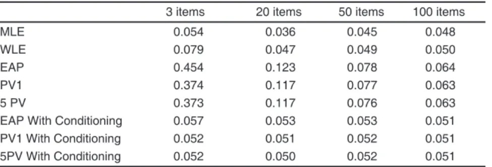
between-school and within-school variance for estimating the sampling variance on the mean for instance, was mentioned. The results reported here show that plausible values can provide un-biased estimates of the school and within-school variances if conditioning on the school mean is implemented. Neither the MLEs, WLEs, nor EAPs can be used for this purpose. If the between-school or the within-between-school variances are biased, one might therefore expect biases in the sampling variance on the mean estimates. To express the importance of the bias, the ratio of the standard error estimate on the mean estimate to the stan-dard error was computed.12 This ratio was then multiplied by 1.96 and the a-error computed. If the sampling variance estimate is unbiased, a will be equal to 0.05. If the sampling variance on the mean is underestimated, a will be greater than 0.05. This means that the null hypothesis will be more often rejected than it should be. Values lower than 0.05 mean that the null hypothesis will be less often rejected than expected. One might be pleased with this latter outcome but on the other hand, it increases the Type 2 error, that is accept-ing the null hypothesis when it is false.
Table 4 presents the Type 1 error per simula-tion per type of proficiency estimate. The biggest biases are associated with EAP and PV generated without conditioning on the school mean of the latent proficiency. As the sampling variance on a 12 Strictly speaking one is interested in the ratio of the estimate of the combined sampling and measurement error variance to the between replication variance. This may mean that the following results are based on ratios that are very slight underestimated for the PVs.
mean for a cluster sample mainly depends on the cluster variance, these results reflect the important underestimation of the cluster variance and it demonstrates the importance of the condition-ing. As the EAPs generated with conditioning properly estimate the between-school variance but systematically underestimate the within-school variance, the Type 1 error is only slightly overestimated. PVs with conditioning seem the most appropriate, as this type of estimates can recover both variance in a satisfactory way. Fi-nally, while MLEs and WLEs proved to provide poor estimates of the variances, and one might have expected large inconsistencies in Table 4 for these estimates, clearly this is not the case. As the bias is mostly located at the within-school level, type 1 error for MLE and especially for WLE are quite acceptable.
Simulations: Two
A national or an international assessment, such as PISA, does not only focus on the estima-tion of the proficiency mean for a populaestima-tion or a set of populations. Policy makers may use the outcomes of the assessment to initiate educational reforms supposed to improve the quality and the equity of the educational system.
Therefore, student proficiency estimates are usually related to some student background or behavioral characteristics or with some teacher or school features. In this context, it is important to ensure that the estimates based upon student proficiency estimates are good estimates of the relationship that exists between the latent profi-ciency and the school or student characteristics. Table 4
Type 1 Error Rates
3 items 20 items 50 items 100 items
MLE 0.054 0.036 0.045 0.048
WLE 0.079 0.047 0.049 0.050
EAP 0.454 0.123 0.078 0.064
PV1 0.374 0.117 0.077 0.063
5 PV 0.373 0.117 0.076 0.063
EAP With Conditioning 0.057 0.053 0.053 0.051
PV1 With Conditioning 0.052 0.051 0.052 0.051
As student proficiency estimates are con-taminated by measurement error, it is well known that the first order correlation between student proficiency estimates and any school or student characteristics is biased towards zero (eg Guil-ford, 1954; Fuller, 1987).
Suppose Y is a variable measured without error and q is a second variable measured with error by ˆq then if ˆq = q +e and cov ,
( )
ˆq e =0then it is easy to show that an unbiased estimate of the correlation between Y and q is given by:
ˆ ˆ ˆ Y Y r r r q q qq = (21)
whererqˆY is the observed correlation between Y and ˆq, rqqˆ ˆis the reliability of ˆq, that is
2 ˆ ˆ 2 ˆ . r q qq q s s =
While these conditions hold for the WLE and MLE they do not hold for the EAP. In the case of the EAP, the estimated value and the error, e, are correlated. However Wu and Adams (2002) show that for the EAP a result analogous to (21) holds if rqqˆ ˆ is given by 2 ˆ ˆ ˆ 2. r q qq q s s =
The second simulation intends to examine how well the different types of student proficiency estimates recover the latent correlation between the student proficiency and another characteristic.
As Guilford pointed out, the bias in the cor-relation estimate will depend on the reliability of the instrument. Therefore, as above, simulations were based on 3, 20, 50 and 100 items.
Simple random samples of 2000 students were drawn from a normal latent population distribution with a mean of zero and a standard deviation of one. The number of replicates used for the first simulation was used for the second one. So the results presented below are based on 276 replicates for a test of 3 items, 223 for a test
of 20 items, 220 for a test of 50 items are 21313 for a test of 100 items.
Results
The observed correlations and correlation estimates corrected for attenuation are provided for these simulations in Table 5. The reliability of the MLE and WLE used for the dissatenuation are defined as:
ˆ ˆ 2 ˆ 1 . rqq q s = (22)
For the EAP the dissattentuation was computed using:
2
ˆ ˆ ˆ.
rqq=sq (23)
The reliability of the plausible values was estimated as the mean of the 10 correlations be-tween the five PVs. The average correlation was computed by using the Fisher transformation. Table 5 presents the average of the correlation coefficient estimates14 with their standardized dif-ference between the correlation and the expected value of 0.30.15
As expected, MLE, WLE, EAP and plausible values without conditioning provide biased esti-mates of the latent correlation. The bias is also proportional to the reliability of the test.
The correction for attenuation appears to work less well for the MLE than for WLE. Indeed, with a test of 20 items or higher, the correlation estimate corrected for attenuation is not signifi-cantly different from the generating value while more than fifty items seems necessary to provide an unbiased estimate of the latent correlation with MLE. This is likely due to the outward bias in MLEs.
13 Due to time constraints, the simulation for a test of 100 items is based on 202 replications with no conditioning, 135 replications with conditioning.
14 The Fisher transformation was firstly applied to the correlation estimates. The mean of the transformed correla-tions was computed and then the inverse transformation was applied.
15 The Fisher transformation was also used to test the dif-ference with the expected value.
The correction for attenuation is best for EAP estimated without conditioning. Even with a test of 3 items, the correlation estimate is unbiased. On the other hand, the correction for attenuation does not work for plausible values generated without conditioning.
On average, the MLE, WLE and EAP corre-lation estimates appear to be identical. This result is not surprising, as in the case of a complete test design, MLE, WLE and EAP each associate a common estimate (in logits) to each possible raw score. Nevertheless, as the interval between two possible logit scores from one type of estimate to another one does not depend on a linear relation-ship, slight differences will be observed between the correlation estimates.
Plausible values with conditioning provide unbiased estimates of the latent correlation, regardless the number of items in the test. On the other hand, due to the underestimation of the total variance, and more specifically the underes-timation of the residual variance, EAP estimates systematically overestimate the latent correlation. As the bias of the residual variance is a function of the reliability, then the product of the observed correlation by the reliability appears to be a satis-factory way of correcting this overestimation. We have not however yet proved this result. In our example, this would give correlation estimates of
0.280, 0.297 and 0.299 respectively for a test of 3, 20 and 50 items.
Discussion and Conclusion
In the PISA 2000 international database, two types of proficiency estimates were included: Weighted Maximum Likelihood Estimates and Plausible Values. Each student who took part in the assessment has at least results on the combined reading scale and the three reading subscales (re-trieving information, interpreting and reflecting) and about 5/9 of the assessed students students also have proficiency estimates in mathematics and/or in science.
With an average test length of 60 items, it follows that student proficiency estimates for the reading subscales, the mathematics scale and the science scale are based on a small set of items (typically between 15 and 20).
As the database is currently widely used for secondary analysis, it is important to ensure that the type of proficiency estimates returned mini-mises the risk of bias.
PISA 2000 data were collected through a complex sampling design. In most cases, schools were firstly drawn and then students were ran-domly selected. Goldstein (1987), Bryk and Raudenbush (1992) brought to our attention the importance of recognising the hierarchical struc-Table 5
Means of Correlation estimates
3 items 20 items 50 items 100 items
Mean Z Mean z Mean z Mean z
MLE 0.176 –99.88 0.262 –30.75 0.283 –14.40 0.291 –6.59 WLE 0.175 –100.87 0.262 –30.28 0.283 –14.25 0.292 –6.53 EAP 0.176 –99.91 0.263 –29.47 0.283 –14.09 0.292 –6.43 PV1 0.105 –160.76 0.230 –52.00 0.268 –26.97 0.283 –13.06 5 PV 0.105 –146.51 0.231 –51.95 0.268 –26.58 0.283 –12.61 MLE corrected 0.272 –14.15 0.316 9.30 0.306 4.46 0.304 2.35 for attenuation WLE corrected 0.248 –26.81 0.299 –0.66 0.300 0.16 0.301 0.49 for attenuation EAP corrected 0.299 –0.49 0.299 –0.88 0.299 –0.69 0.300 –0.28 for attenuation PV1 corrected 0.178 –62.70 0.261 –25.73 0.283 –13.43 0.291 –6.51 for attenuation
EAP With Conditioning 0.478 47.68 0.339 24.61 0.317 12.88 0.309 5.86 PV1 With Conditioning 0.298 –1.01 0.298 –1.43 0.301 0.40 0.300 0.32 5PV With Conditioning 0.297 –1.18 0.299 –0.51 0.300 0.26 0.300 0.15
ture of the data. The first simulation has shown that the hierarchical structure of the data needs to be taken into account not only when secondary analyses are performed but also when student proficiency estimates are generated. The results show the superiority of the plausible values with conditioning for recovering the between-school and within-school variances.
The second simulation compares the ef-ficiency of the different types of estimates for recovering a latent correlation. It appears that WLE will provide unbiased estimates if the test has at least about 20 items. But this correlation needs to be attenuated and users of the database might not be aware of this requirement. Plausible values allow the users to safely avoid this correc-tion. Nevertheless, the generation of plausible values requires a careful conditioning; otherwise their superiority will be limited to the estimation of the total variance and percentiles.
Acknowledgement
The authors would like to make a special ac-knowledgement to Claus Carstensen who made a significant contribution to the scaling of the PISA 2000 data. We would also like to thank Norman Verhelst for his wonderful advice and support.
References
Adams, R. J., and Wilson, M. R., and Wang, W. (1997). The multidimensional random coefficients multinomial logit model. Applied Psychological Measurement, 21, 1-24 Adams, R. J., and Wu, M. L. (Eds.) (2002) PISA
2000 Technical Report. OECD, Paris. Adams, R. J., Wilson, M. R., and Wu, M. L.
(1997) Multilevel item response modelling: An approach to errors in variables regression. Journal of Educational and Behavioral Sta‑ tistics, 22, 47-76.
Beaton, A. E. (1987). Implementing the new de‑ sign: The NAEP 1983‑84 Technical Report. (Report No. 15-TR-20). Princeton, NJ: Edu-cational Testing Service.
Bryk, A. S., and Raudenbush, S. W. (1992). Hi‑ erarchical linear models: Applications and data analysis methods. Newbury Park: Sage. Chang, H., and Stout, W. (1993). The asymptotic
posterior normality of the latent train in an IRT model. Psychometrika, 58, 37-52.
Goldstein, H. (1987). Multilevel statistical mod‑ els. London: Edward Arnold.
Guilford, J. P. (1954) Psychometric methods. New York: McGraw-Hill.
Fuller, W. (1987). Measurement error models. New York: Wiley.
Littell, R. C., Milliken, G. A., Stroup, W. W., and Wolfinger, R. D. (1999). SAS system for mixed models. Cary, NC: SAS Institute.
Macaskill, G., Adams, R. J., and Wu, M. L. (1998). Scaling methodology and procedures for the mathematics and science literacy, advanced mathematics and physics scales. In M. Martin and D. L. Kelly (Eds.) Third inter‑ national mathematics and science study. Tech‑ nical Report Volume 3: Implementation and Analysis. Boston College: Chestnut Hill, MA. Mislevy, R. J. (1991). Randomization-based in-ference about latent variables from complex samples. Psychometrika, 56, 177-196. Mislevy, R. J., Beaton, A. E., Kaplan, B., and
Sheehan, K. M. (1992). Estimating population characteristics from sparse matrix samples of item responses. Journal of Educational Mea‑ surement, 29, 133-161.
Mislevy, R. J., and Sheehan, K. M. (1989). In-formation matrices in latent-variable models. Journal of Educational Statistics, 14(4), 335-350.
Organization for Economic Co-operation and Development. (2001). Knowledge and skills for life: First results from PISA 2000. Paris: OECD Publications.
Organization for Economic Co-operation and Development. (2004).Learning for tomorrow’s world: First results from PISA 2003. Paris: OECD Publications.
Rubin, D. B. (1987) Multiple imputations for non‑response in surveys. New York: John Wiley and Sons.
Thomas, N. (2000). Assessing model sensitivity of the imputation methods used in the national assessment of educational progress. Journal of Educational and Behavioral Statistics, 25, 351-371.
Thomas, N., and Gan, N. (1997). Generating multiple imputations for matrix sampling data analyzed with item response models. Journal of Educational and Behavioral Statistics, 22, 425-446.
Warm, T. A. (1985). Weighted maximum likeli-hood estimation of ability in item response theory with tests of finite length. Technical Report CGI‑TR‑85‑08. Oklahoma City, OK: U.S. Cost Guard Institute.
Wu, M. L., and Adams, R. J., (2002, April). Plausible Values: Why they are important. Paper presented at the International Objective Measurement workshop, New Orleans, LA. Wu, M. L., Adams, R. J., and Wilson, M. R.
(1997). ConQuest: Multi-aspect test software [Computer program]. Camberwell: Australian Council for Educational Research.