Performance Study of an Overlay Approach to Active Routing in Ad Hoc Networks

(1)

Performance Study of an Overlay Approach to

Active Routing in Ad Hoc Networks

Sandrine Calomme and Guy Leduc

Research Unit in Networking

Electrical Engineering and Computer Science Department University of Li`ege, Belgium

Email: _{{calomme,leduc}@run.montefiore.ulg.ac.be}

Abstract— We motivate the use of the active technology

for routing in ad hoc networks.

We present an active architecture where passive and active nodes can operate together, avoiding any change in the legacy muti-hop routing protocol they use.

We detail a basic reactive protocol which can be used to build any overlay on top of an ad hoc network. We model it as an active application called Re-Active Routing (RAR).

RAR provides dynamic routing in dense and sparse active overlays. We investigate its performance in static and dynamic environments and show that it depends substantially on the active range, i.e. on the allowed maximal number of hops between two active nodes. For a well-chosen active range, RAR achieves good performance even if the mobility level is high and the overlay density is as low as 12.5 %.

I. MOTIVATION

This work is based on the conviction that the active and ad hoc technologies are complementary for building a very flexible network where users do not need a third party to communicate. An ad hoc network is defined as a collection of wireless mobile nodes dynamically forming a temporary network without the use of any existing network infrastructure or centralized administration [1]. In this environment, the only way for a node to reach another one which is not in its range is to use a multi-hop path passing through intermediate nodes. Various multi-hop routing protocols have been developed. They can first be classified in three categories: proactive, reactive and hybrid. Each class has its own assets; one should prefer a proactive protocol if the nodes mobility is low, a reactive one if the mobility is high. Some hybrid protocols are well-suited for large networks while some reactive protocols are not. Even if we only consider the reactive class, there is still a large panel of protocols, each more or less adapted to the network conditions and to the application needs, in terms, for example, of energy

saving, path stability or control traffic amount. In order to communicate, all the nodes must of course share the same routing protocol. This is not a restriction in the context of sensor networks or disaster relief and more generally in situations where all the nodes are intended to be used for a specific application : the environment is known as well as the user’s needs and resources. However, within an heterogeneous environment, in terms of nodes resources (bandwidth, computing, memory and energy) and user’s needs, if the network conditions are not known a priori or varying, the requirement of choosing a routing protocol and imposing it to all nodes is a limitation. This can be overcome thanks to the active technology. With an active or programmable network element, it is possible to load new protocols or ser-vices automatically, and to remove protocols or serser-vices that are no longer useful, without service interruption. A reactive routing protocol could be fully injected or configured by an end user, following its needs, and it could be adapted to the network conditions and to the available resources in each intermediate node. Moreover, the active technology would allow a direct use of new protocols, avoiding the time consuming standardization process. Finally, thanks to it, nodes would not have to store plenty of protocols for other user’s needs.

We assume that ad hoc networks, if spreading, will be progressivily deployed in a classical way, on passive nodes, after standardization of a few routing protocols. We present an architecture which allows the progressive introduction of the active technology by ad hoc users, simply upgrading software on their wireless devices. We adopted an overlay approach. All hosts share a common legacy routing protocol. Some users install an active plat-form on their node. These active nodes use the passive routing protocol for communication with neighbours. To communicate with farther nodes, a routing process is run as an active application.

(2)

The framework we introduce is composed of an active architecture for ad hoc nodes and an elementary routing active application. It has been developed with the fol-lowing objectives in view :

• dynamic reactive routing between active nodes • transparent co-existence of active and legacy

net-work nodes

• operation in geographically dense and sparse net-works

• operation with high and low ratio of active nodes in the network

We do not intend to present a new efficient protocol for ad hoc networks. The active application we simulated implements a basic route discovery mechanism very similar to the one of AODV [2]. We use it to study the feasability and the efficiency of re-active applications developed according to our architecture.

This preliminary study aims at laying the founda-tions for easy extensions of our framework, leading to customized, efficient active applications. One could, for example, add mechanisms for gossiping [3], multiple paths discovery and load balancing [4] or cooperative caching of packets [5].

II. RELATEDWORK

An active and ad hoc node architecture is presented in [6], where the forwarding functionality is separated from the setup and monitoring ones. In this approach, every mobile node is turned into an active router. Active packets create private forwarding entries through which passive data packets are routed without any active packet processing overhead. In order to distinguish packets belonging to different private forwarding circuitry, an additional packet header field is needed, defined by the ”Simple Active Packet Format” (SAPF). All packets, active and passive, must be encapsulated in this new header which contains a selector indicating to SAPF nodes how to process the packet. This forms a pro-grammable infrastructure supporting different network personalities that share the route table resource, so a multitude of routing protocols can be chosen among and run in parallel. The efficiency of SAPF has been shown by real tests on delay-sensitive audio traffic.

In [7], the authors argue that future mobile networks are the ideal target for the adoption of active networks because of their big need in flexibility. They present sev-eral applications that would benefit of this architecture and, in particular, assert that activity would be useful in ad hoc networks for a context-aware choice of the most

appropriate routing protocol and for integration with cel-lular networks. In this architecture, the programmability is applied to all layers of the mobile devices and also to their cross-layer interfaces.

Several researchers have also proposed some practical use of the active technology in ad hoc networks. In [8], a network discovery mechanism using capsules improves the DSR [9] performances by pro-activily updating the route caches. Simulations show that route failures and control traffic are reduced and that route changes take less time. In [10], the same protocol, ADSR, is improved for congestion avoidance : when visiting the nodes, the capsules observe the routing queue length and compute a new route for flows which are suffering congestion. Simulation results show that ADSR significantly im-proves TCP performance. In [11], each node observes environmental conditions and uses a fitting function to detect when it would be desirable to switch from DSR to AODV and from AODV to DSR. When this happens, it warns its neighbours and they vote to switch all together or not. The node activity is used to load code, when necessary, from a neighbour using a different protocol.

In all these works, the basic ideas of integrating the active and ad hoc technologies are similar to ours but they deal with fully active networks.

III. RE-ACTIVEROUTING OVERVIEW

A. Architecture

We instantiate the general architectural model de-scribed in [12]. In this framework, an active network consists of a set of nodes — not all of which need to be active — connected by a variety of network technologies. Users obtain end-to-end services from the active network via Active Applications (AAs). The AAs are written by the network users according to their needs and dynamically downloaded on the nodes where they are required.

Each active node runs a Node Operating System (NodeOS) and one or more Execution Environments (EEs). The NodeOS is responsible for managing local resources and provides a packet-forwarding technology for communication between EEs. The EEs send the packets built by a local AA and deliver them to their peers on the appropriate distant active node thanks to the communication channels supplied by the NodeOS. Each of them also implements a virtual machine that interprets active packets that arrive at the node.

The communication paths between active nodes are discovered by an Active Application we designed and called Re-Active Routing (RAR). At the NodeOs level,

(3)

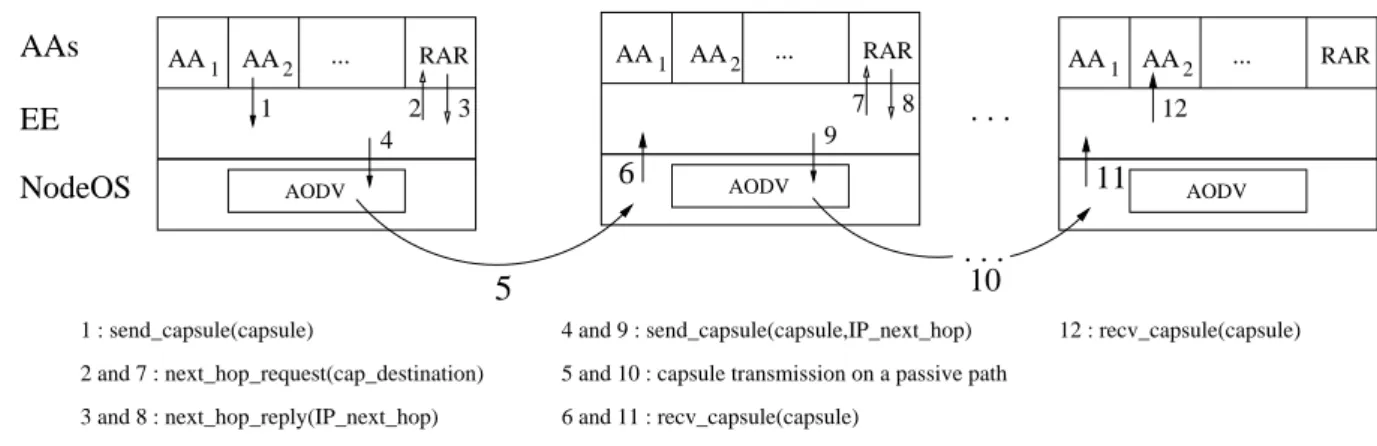
AA₁ AA₂ AA₁ AA₂ AA₁ AA₂ AODV ... 12 RAR AODV ... RAR 1 2 3 4 5 AODV ... RAR 7 8 9 AAs EE NodeOS . . . 10 11 6 . . . 2 and 7 : next_hop_request(cap_destination) 3 and 8 : next_hop_reply(IP_next_hop)

1 : send_capsule(capsule) 4 and 9 : send_capsule(capsule,IP_next_hop) 5 and 10 : capsule transmission on a passive path 6 and 11 : recv_capsule(capsule)

12 : recv_capsule(capsule)

Fig. 1. Capsule transmission main steps from source to destination

we only assume the use of a “bare” legacy ad hoc routing algorithm for the communication between two successive EEs on the routes created by RAR.

The general flow of packets through an active node using RAR is shown in figure 1. When an active packet is generated by an AA, the receiving EE asks RAR the IP address of the next active hop on the path to the final destination of the packet. When this is known, the EE gives the packet to the NodeOS which will use its legacy ad hoc routing protocol, in our simulation model AODV [2], to forward the packet. When an EE receives an active packet, it first looks its active destination field. If it is the local node, it delivers the packet to the appropriate AA relying on the active protocol identifier field. If it is a distant node, it asks RAR to determine the next hop as described above.

B. RAR route construction

RAR is a reactive protocol : an active route is created only when it is needed by an AA. As for AODV, route discovery follows a route request/route reply query cycle. An active source node in need of a route broadcasts an Active Route Request (ARREQ) packet accross the network. Any node with a current route to the destina-tion, including the destination itself, can respond to the ARREQ by sending an Active Route Reply (ARREP) back to the source node. Once the source node receives the ARREP, it can begin sending data packets along this route to the destination. To prevent unnecessary network-wide dissemination of ARREQs, the originating node uses an expanding ring search technique. It initially uses a small active Time To Live (ATTL), in case the destina-tion node is located close to itself. If necessary, it later sends other ARREQs with a progressivily increasing ATTL, until it receives an ARREP. The maximum ATTL value is bounded because the destination node can really

be unreachable.

In the AODV protocol, the route reply (RREP) mes-sages are sent in unicast, following the reverse route built on the intermediate nodes. In RAR, the ARREP messages also follow the reverse path, but they are broadcast. Indeed, if an ARREP is to be unicast from one active node to its predecessor P, the underlying passive reactive protocol may not know a passive path to P and may have to search a route before forwarding it, which would generate unnecessary delays1.

When an active node receives an ARREP, it analyzes the next active hop field. If this field contains its identity, it is the good predecessor so it processes the capsule. If not, it simply drops it.

Ad hoc random access MAC protocols often treat unicast and broadcast packets differently. Unicast packets are preceded with MAC layer control frames, such as RTS/CTS followed by ACK, to ensure that the desti-nation receives the unicast packets. Broadcast packets, on the other hand, are sent blindly without any control frames to assure the availability of the destinations [14]. This makes broadcast packets more likely to be lost than unicast ones. To avoid ARREP losses, the reception of an ARREP is confirmed by the emission of an ARRACK. Two retransmissions of an ARREP are allowed. The ARRACKs are unicast; this is more reliable, does not increase the route construction time and finally opens the successive passive path pieces between consecutive EEs on the global active path, decreasing the end-to-end transmission delay of the first active data capsule.

RAR can work as well in sparse as in dense mobile 1_{Notice that this is an optimization for passive reactive routing}

protocols. If, for example, we had chosen a proactive protocol like DSDV [13], it should have been more appropriate to unicast the ARREPs because the passive path would have been immediately available.

(4)

RREQ

S

D

(a) Route requests propagation

RREP

S

D

(b) Route replies propagation Fig. 2. AODV route discovery process

active environments. The ARREQ and ARREP messages are encapsulated in IP broadcast packets with the Time To Live field set to a constant parameter called the active

range and denotedAR. The active range is the maximum

number of hops on the optimal path linking two active neighbours. If AODV uses an optimal path between two active neighbours, the active capsules flowing between them will not go through more than the _{AR − 1} pas-sive nodes. Because AODV sometimes provides paths a little longer than the optimal one, we will assume, for small active ranges, that the maximum number of passive nodes traversed by an active capsule between two active neighbours is the active range. Figures 2 and 3 illustrate respectively the AODV and RAR route discovery processes on a tiny topology. The active range is set to two.

C. RAR route maintenance

Because nodes are moving, link breaks are likely to occur, which in turn breaks passive paths between successive active nodes.

As AODV, RAR can operate in two modes : hello or active link break detection.

In the hello mode, each active node lying on an active route2 emits at regular intervals a broadcast AHELLO capsule carrying its EE identity. The Active Time To Live

2

In the AODV terminology [15], an active route is a route towards a destination that has a routing table entry marked as valid, because it has been recently created or is successfully used by a data packets flow. Only active routes can be used to forward data packets. The term active has thus a different meaning when related to a route and to a node; the reader will have to infer it from the context.

passive node active node ARREQ

S

D

(a) Active route requests propagation

passive node active node ARREP ARRACK S D

(b) Active route replies and route reply aknowledgments propagation

Fig. 3. RAR route discovery process (AR = 2)

field of the capsule is set to one and the Time To Live field of the IP packet which carries it is set to the active range. A predecessor not receiving these capsules knows that the node can no more be used as next active hop and informs the source that the active route is broken.

In the active link break detection mode, when the source of a passive routing path receives a route error message (RERR), the EEs using this path are informed. This is the only modification we impose to AODV, and it is necessary only in this mode.

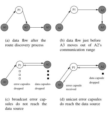
In AODV, when a link break in an active route occurs, the node upstream of the break broadcasts a RERR message containing a list of all the destinations which are now unreachable due to the loss of the link. In RAR, we send a separate unicast message to each of the active neighbours affected by the break. This is less bandwidth-efficient and, if the flow is uni-directional, the source is later notified of the break in this way, but necessary with the active link break detection mode. If we do send broadcast ARERR messages, there exist scenarios where all successive ARERR messages sent by an active node are lost. Let us for example assume that the active neighbour range in the sequence of events illustrated by figure 4 is set to one. Consider the active path A1-A2-A3 in part a of this figure. A2 is in the range of A1 but AODV has found a two hop route between them, going through the passive node P1. In part b, A2 has moved out of range of A1 but the data capsules continue to be delivered because the passive route A1-P1-A2 is still valid. In parts c and d, the passive path between A3 and

(5)

A3 A1 A2

P1

(a) data flow after the route discovery process

A3 A1

A2 P1

(b) data flow just before A3 moves out of A2’s communication range data capsules dropped P1 A1 A2 error capsules dropped

(c) broadcast error cap-sules do not reach the data source data capsule dropped P1 error capsule received A2 A1

(d) unicast error capsules do reach the data source

Fig. 4. Error capsules must be unicast

A2 is broken, so A2 sends a route error capsule. If this capsule is broadcast, as in part c, its Time To Live field is set to the active range value, one. When P1 receives the broadcast packet, it drops it because the Time To Live, after decrement, is null. If the capsule is unicast, as in part d, it does reach A1.

Table I summarizes the AODV and RAR control messages type and emission mode.

IV. SIMULATIONS

The network is composed of active and passive ad hoc nodes. We call the ratio of active nodes over the total amount of nodes the overlay density. We study the impact of the network density and diameter, of the overlay density and of the mobility level on the protocol. We developed an EE environment for the ns-2 simu-lator [16] with the extensions from the Monarch Project [17]. We use the AODV implementation provided with ns-2.26.

We first analyze RAR performance with static nodes only and then study the mobility impact.

A. Static networks

1) Static testbed description: We operate with static and uncongested nodes. The nodes transmitting range is set to 250 meters. Two nodes are said to be connected if there exists a multihop path between them.

With a first set of experiments, we study the influence of the network density on performance. The nodes are

0 0.2 0.4 0.6 0.8 1 16 32 64 128 256 Av. connectivity () Nodes number ()

Varying geographical density Varying field length

PSfrag replacements

N etwork density/Dref()

N etwork diameter/dref()

N etwork density /Dref() N etwork diameter /dref() Overlay density () Overlay density () 1/4 1/2 1/√2 1 √2 2 4 1/4 Dref 1/2 Dref 1 Dref 2 Dref 4 Dref 1/2 dref 1/√2 dref 1 dref √2 dref 2 dref

(a) Average connectivity

1.5 2 2.5 3 3.5 4 4.5 5 5.5 6 16 32 64 128 256

Av. path length (hop)

Nodes number ()

Varying geographical density Varying field length

PSfrag replacements

(b) Average path length

Fig. 5. Static testbed: Connectivity and path length characteristics versus nodes number

distributed uniformly and independently in a 1000 meter long square field. The density obtained with 64 nodes is taken as a reference and noted Dref. We test densities of 0.25, 0.5, 1, 2 and 4 times Dref by disseminating respectively 16, 32, 64, 128 and 256 nodes in the field. In order to study the network diameter effect, we construct a second set of topologies. In this set, the network density is equal to the reference density Dref for all experiments. The network diameter obtained with 64 nodes is taken as a reference and noteddref. We also use 16, 32, 64, 128 and 256 nodes, but in fields length respectively of 500, 707, 1000, 1414 and 2000 meters in order to maintain a constant network density. We thus handle topologies with a diameter of 1/2, 1/√2 _,1,√2

and 2 times dref.

We generate 50 different topologies for each network density and diameter. We then randomly choose 10 pairs of connected nodes for each of them.

The average percentage of connected nodes pairs for both sets of experiments is depicted in figure 5(a). The number of nodes employed in the first set of experiments determines the network density. This has a strong impact

(6)

TABLE I

AODVANDRARCONTROL MESSAGES

AODV packets RAR capsules

Message type Emission mode IP TTL Emission mode Active TTL IP TTL Route Request Broadcast [1, N ET D] Broadcast [1, AN ET D] AR

Route Reply Unicast N ET D Broadcast AN ET D AR

Route Reply Acknowledgment - - Unicast 1 AR + 1

Route Error Broadcast 1 Unicast 1 AR + 1

Hello Broadcast 1 Broadcast 1 AR

N ET D = estimated network diameter AN ET D = estimated active network diameter

on the global average connectivity. Above the reference density, all pairs of nodes are connected. At half of the reference density, about 80 % of the pairs are connected and dividing again the density by two leads to a very poor connectivity of about 35 %. The first set thus allows us to study the protocol in sparse and dense networks. In the second set of experiments, the network density is constant and the figure indicates a global connectivity almost equal to 100 % at all network diameters.

The path length characteristic of the two sets is drawn in figure 5(b). The network diameter strongly affects the global average optimal path length, while the network density has almost no effect on it. For the first set, the path length drops in the outmost left part of the figure because we chose connected pairs of nodes. Connected nodes are seldomly far away from each other in very sparse networks.

The parameters of the two sets of experiments em-ployed in the static study are summarized in table II. The graphs presented below are divided following these sets; we analyze the network density and the network diameter influence on performance at various overlay densities. The values assigned to the overlay density are

12_{.5, 25, 37.5, 50, 62.5, 75, 87.5 and 100 percent. As}

there are fifty scenarios and ten connections used at each network density and diameter, all the points presented are an average on five hundred runs.

At the beginning of each simulation, the source tries to send one UDP datagram containing a 512 bytes data payload 3_{. Simulations are stopped after 50 seconds. If}

the packet has been received, the simulation is said to be successful.

3_{In simulations using AODV alone, the datagram payload is exactly}

512 bytes. In simulations testing RAR over AODV, the source tries to send a capsule with a data payload of 512 bytes. We modelled ANEP [18] capsule headers, which are eight byte long, so the datagrams payload is in fact equal to 520 bytes.

TABLE II

STATIC TESTBED TWO SIMULATION SETS

Set 1 Set 2

Network density (Dref) 0.25, 0.5, 1, 2, 4 1

Network diameter (dref) 1 1/2, 1/√2, 1, √2, 2

Overlay density (%) 12.5, 25, 37.5, 50, 62.5, 75, 87.5, 100

2) Static testbed goals: In our reactive approach of active routing, there is no neighbour probe before a route is needed. Active neighbours are implicitly detected during route discoveries. As long as the probability of finding a route composed uniquely of active nodes is high, it is sufficient to use all physical neighbours that are active as next hops. The Time To Live field of the ARREQ packet, the active range (AR), is set to one. This makes overlay neighbours process and eventually resend the ARREQs, while the passive neighbours simply drop them. However, if the network or overlay density is not high enough, a unitary active range may not be sufficient to allow communication. In the static study, we run each simulation with an increasing active range until it becomes successful and then log the performance obtained : path length, control traffic and delivery delay. We thus show RAR performance in the ideal case, i.e. when the active range used is the minimum one allowing to find a route between the source and destination nodes. The network characteristics, density and diameter, and the overlay density effect on performance are pointed out. We take the AODV protocol as a reference for evaluating RAR.

3) Control traffic: The number of control packets needed to send the first data packet is often referred to as the normalized routing load.

We include in the control traffic of RAR all AODV packets emitted to build passive routes between

(7)

succes-0 1 2 3 4 5 6 0.1 0.2 0.3 0.4 0.5 0.6 0.7 0.8 0.9 1

Control traffic comparison RAR/AODV ()

Overlay density () PSfrag replacements

(a) Varying network density

0 1 2 3 4 5 6 0.1 0.2 0.3 0.4 0.5 0.6 0.7 0.8 0.9 1

Control traffic comparison RAR/AODV ()

N etwork diameter/dref ()

(b) Varying network diameter

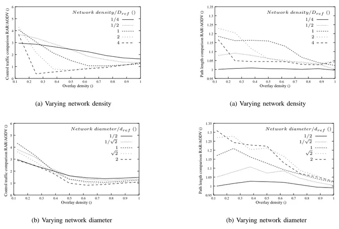
Fig. 6. Static study: control traffic overhead induced by RAR in comparison with AODV

sive active nodes.

Figure 6 shows the RAR overhead normalized routing load, which we define as the ratio between the RAR (over AODV) normalized routing load and the AODV one. The normalized routing load of AODV, taken as reference for evaluating RAR, corresponds to the control traffic employed by AODV to establish the communication in a pure passive network and, given a topology and a source-destination pair, is the same at all overlay densities.

At high and moderate network densities, a decrease of overlay density first helps reducing the control traffic by performing a kind of natural gossiping [3]. Then, a reduction of overlay density increases the control traffic because longest active ranges are required for finding an active route. The control traffic sensitivity to the overlay density is stronger at high network densities. At the lowest network density, a decrease in overlay density does not help because the number of rebroadcast ARREQ is low, even if the network is totally active.

The distance between the source and destination is the most determinant factor increasing the absolute normal-ized routing load, for RAR as for AODV. However, it

0.95 1 1.05 1.1 1.15 1.2 1.25 1.3 1.35 0.1 0.2 0.3 0.4 0.5 0.6 0.7 0.8 0.9 1

Path length comparison RAR/AODV ()

0.95 1 1.05 1.1 1.15 1.2 1.25 1.3 1.35 0.1 0.2 0.3 0.4 0.5 0.6 0.7 0.8 0.9 1

Path length comparison RAR/AODV ()

N etwork density/Dref ()

N etwork density /Dref () N etwork diameter /dref () Overlay density () Overlay density () 1/4 1/2 1/√2 1 √2 2 4 1/4 Dref 1/2 Dref 1 Dref 2 Dref 4 Dref 1/2 dref 1/√2 dref 1 dref √2 dref 2 dref

(b) Varying network diameter

Fig. 7. Static study: average path length comparison (RAR/AODV)

does not influence a lot the RAR overhead normalized routing load.

4) Path length: As the overlay density decreases, the active route followed by the packet may deviate from the shortest passive route.

The possibility to build non optimal paths of RAR, between the source and destination active nodes, and of AODV, between successive active nodes on the route found by RAR, are summed. This sub-optimality strengthens when the distance between source and des-tination is long.

These two effects are shown by figure 7, where the ratio of the average path lengths obtained with RAR and AODV is drawn. The overhead average path length induced by RAR over AODV seldomly exceeds 30 %.

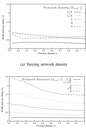
5) Delivery delay: The last performance parameter to study is the delivery delay. This can be divided into two parts: the time necessary for a node to find a route and for the packet to progress on this route, which we respectively call the route discovery delay and the path delay. Because there is only one capsule sent, the route discovery delay constitutes the main part of the total transmission delay in the static study.

(8)

0 0.5 1 1.5 2 2.5 0.1 0.2 0.3 0.4 0.5 0.6 0.7 0.8 0.9 1 Overlay density ()

RAR delivery delay (s)

PSfrag replacements

0 0.5 1 1.5 2 2.5 0.1 0.2 0.3 0.4 0.5 0.6 0.7 0.8 0.9 1

(b) Varying network diameter Fig. 8. Static study: delivery delay

The network diameter has a big influence on the AODV delivery delay. As shown in figure 8, this is also the case for RAR. There are two reasons for it. Firstly, the network diameter increases the average number of ring searches. Secondly, it raises the average control traffic which in turn lengthens the contention delay during the route requests propagation. When the path length is constant, the variation of the delivery delay is weaker but we can observe that it has the same shape as the overhead control traffic. In summary, the total delivery delay in the static study is very close to the average route discovery delay, which depends on the network diameter and on the amount of control traffic.

We also compared the total delays obtained with RAR and AODV. In the static study, the RAR overhead delay increases from 25 to 100 % when the overlay density diminishes, independently of the passive topology char-acteristics.

B. Dynamic networks

1) Dynamic testbed description: The common param-eters for all simulations in this testbed are listed in table III.

TABLE III

DYNAMIC TESTBED COMMON PARAMETERS

Simulation Parameter Value Simulator ns-2.26 Data Packet Size 512 bytes payload Node Max. IFQ length 50

Packet rate 4 per second Nodes transmitting range 250 m

Field length 1000 m

Nodes number 64

Connections number 1 Simulation duration 600 s

Number of trials 20

We now work at the reference geographical density, vary the overlay density and the mobility level. As for the static tests, we explore overlay densities of 12.5, 25, 37_{.5, 50, 62.5, 75, 87.5 and 100 percent. We generate}

10 different topologies for each mobility level. We also use one source-destination pair per simulation to analyze an uncongested environment. For mobility, we apply the random waypoint model [9]. The simulations duration is 600 seconds. Each node is at rest at the beginning of the simulation for pausetime seconds, then choses

a random destination on the field and moves to it with a randomly and uniformly chosen speed in the range of 0 to 20 m/sec. When it has reached its destination, it pauses again for pausetime seconds, then moves

again, and so on. We vary the pause time to simulate different mobility levels : 0, 30 , 60, 120, 300 and 600 seconds. A zero pause time indicates that nodes are continuously moving while a 600-second pause time means that nodes are at rest for the entire simulation duration. We randomly chose 2 pairs (srci,dsti) in each topology as test connections. As there are ten scenarios and two connections used at each mobility level, all the points presented in the graphs below are an average on twenty runs.

In this environment, physical as well as active links can break. In this paper, AODV and RAR both operate in the link break detection mode.

2) Dynamic testbed goals: In the dynamic testbed, for each simulation, we set an active range value a priori. This means that active routes may not be found, even if the chosen source and the destination are connected at the passive level. A source which does not find a route after three consecutive full ring searches separated by ten seconds intervals, estimates that the network conditions are bad and stops trying to send data. The simulation

(9)

ends and the performance are logged. In this situation, the control traffic is high and the percentage of packets received low. If a route is always found, the simulation is stopped after 600 seconds and the performance logged. This means that the control traffic and delay overhead costs observed in the dynamic study are higher than the ideal ones analyzed with the static study.

In the dynamic study, we first investigate the qualita-tive effect of mobility on RAR over AODV, compared to AODV alone. We then analyze the impact of a bad active range choice on performance by comparing the results obtained for a pausetime of 600 seconds to the ones obtained in the static study. We finally point out the overlay density effect on performance once again.

We do not expect to obtain exact average performance measures with the random waypoint mobility model [19]. All the analyses in this section are qualitative. Moreover, the random waypoint model should impact AODV and RAR, whose principles are very similar, in the same way, and to limit the bias it introduces, we use the same maximum speed value and simulation duration for all tests [19], [20]. We consequently assume that all conclusions we make on the basis of the following comparisons would remain valid with a mobility model that keeps the average speed, the number of neighbours and the node density uniformity invariant [20], [21]. This will be checked in future work.

3) Percentage of packets received: Figure 9 compares the percentage of packets received using AODV and RAR with an active range set to 1, 2 and 3 hops.

In each graph, the curve at a 600-second pause time, related to static nodes, can be interpreted as an evaluation of the connectivity at the active level. At the reference geographical density, the probability of finding a passive route between the source and destination nodes is very high. This is not the case for active routes. An active route can be found only if there is a passive path between the source and destination nodes on which active nodes are separated by a number of hops lower or equal to the active range value. If the overlay density or the active range is not high enough, an active route may not exist. With a unitary active range, if the overlay density is below 60 %, the connectivity at the active level drops and the percentage of capsules received is very low, compared to AODV. This shows that a unitary active range would not be a pertinent choice for the throughput in a large panel of network and overlay densities, and consequently that an overlay approach is relevant for sparse active networks. We will not show the results obtained with a unitary active range for other

0.95 0.96 0.97 0.98 0.99 1 0 100 200 300 400 500 600

Av. packets received percentage ()

Pause Time (s) PSfrag replacements

N etwork density /Dref() N etwork diameter /dref() Overlay density () Overlay density () 1/4 1/2 1/√2 1 √2 2 4 1/4 Dref 1/2 Dref 1 Dref 2 Dref 4 Dref 1/2 dref 1/√2 dref 1 dref √2 dref 2 dref (a) AODV 0 0.2 0.4 0.6 0.8 1 0.1 0.2 0.3 0.4 0.5 0.6 0.7 0.8 0.9 1 600 seconds 0 second 30 seconds 60 seconds 120 seconds 300 seconds Pause time

(b) RAR - Active range = 1

0 0.2 0.4 0.6 0.8 1 0.1 0.2 0.3 0.4 0.5 0.6 0.7 0.8 0.9 1

Overlay density () 0 second 30 seconds 60 seconds 120 seconds 300 seconds 600 seconds Pause time PSfrag replacements

(c) RAR - Active range = 2

0 0.2 0.4 0.6 0.8 1 0.1 0.2 0.3 0.4 0.5 0.6 0.7 0.8 0.9 1

Overlay density () 0 second 30 seconds 60 seconds 120 seconds 300 seconds 600 seconds Pause time PSfrag replacements

N etwork density /Dref () N etwork diameter /dref () Overlay density () Overlay density () 1/4 1/2 1/√2 1 √2 2 4 1/4 Dref 1/2 Dref 1 Dref 2 Dref 4 Dref 1/2 dref 1/√2 dref 1 dref √2 dref 2 dref

(d) RAR - Active range = 3

(10)

performance analyses.

With an active range value of two, except for the low-est overlay density, the active network is fully connected and the percentage of capsules received is above 80 %, at all mobility rates. In a pure active network, the per-centage of packets received with RAR varies from 100 to 94, instead of 97 with AODV alone. This difference is due to longer route breakage detection time and periods during which an active route cannot be found. When the overlay density decreases, the opportunity of finding an active route also does and the percentage of packets received is more affected by frequent route breakages than in pure active networks.

At the lowest overlay density, an active range value of three improves a lot the percentage of capsules received. However, a longer active range does not only increase the connectivity at the active level, it also results in bigger control traffic and extended route discovery delays during which some capsules may be dropped from the route waiting queue: for overlay densities between 25 and 50 %, the througphut obtained with an active range of only two is better.

We can also observe that, as for AODV, the RAR throughput is first damaged by the quantity of moving nodes, then the mobility helps finding routes between source and destination. This is particularly observable at low overlay densities, because the connectivity at the active level is low.

In summary, the quantity of mobility affects more RAR than AODV but, if the active range value is adapted to the network conditions, the capsules throughput is over 80 % in all cases.

4) Control traffic: Figure 10 shows the ratio of the control traffic induced by RAR over AODV and the one of AODV alone.

The overhead control traffic is not high when the overlay density is very high or very low. However, for intermediate overlay densities, it can be very big. In a pure active network, whatever the mobility rate, the control traffic induced by RAR is similar to the AODV one because the diffusion control of the broadcast messages is the same. In a very sparse active network, the propagation of the broadcast capsules, embedded in broadcast packets, is controlled by the passive nodes. The IP Time To Live field of the packets carrying the ARREQs reaches zero before an active node receives and re-broadcasts them. The control traffic is thus low but the received data percentage obtained is weak. For intermediate overlay densities, the ARREQs capsules are received by active nodes. When a capsule is rebroadcast,

0 2 4 6 8 10 12 14 16 18 20 0.1 0.2 0.3 0.4 0.5 0.6 0.7 0.8 0.9 1 30 seconds 60 seconds 120 seconds 300 seconds 600 seconds Pause time 0 second

Control packets comparison RAR/AODV ()

(a) Active range = 2

0 2 4 6 8 10 12 14 16 18 20 0.1 0.2 0.3 0.9 1

Control packets comparison RAR/AODV () _0.4 _0.5 _0.6 _0.7 _0.8 Overlay density () Pause time 0 second 30 seconds 60 seconds 120 seconds 300 seconds 600 seconds PSfrag replacements

N etwork density /Dref () N etwork diameter /dref () Overlay density () Overlay density () 1/4 1/2 1/√2 1 √2 2 4 1/4 Dref 1/2 Dref 1 Dref 2 Dref 4 Dref 1/2 dref 1/√2 dref 1 dref √2 dref 2 dref (b) Active range = 3

Fig. 10. Dynamic study: control traffic comparison (RAR/AODV)

it is embedded in a new IP packet and the neighbouring passive nodes do not drop it, even if they already have received an IP packet containing exactly the same cap-sule. Useless active route requests are thus propagated.

As expected, the control overhead obtained for mo-tionless nodes is higher than in the static study. On first hand, if an active route search procedure ends unsuc-cessfully because the active range is not large enough to enable communication, the source node starts a new ex-panding ring search after ten seconds. This is particularly prohibitive for static nodes, because the sources make three successive unsuccessful route searches before the simulation gets stopped. On the other hand, if the active range used is larger than the optimum one, the control traffic can also increase because of the propagation of unnecessary active route requests. This explains why the control overhead obtained is doubled when using an active range value of three instead of two and why it is so high for overlay densities between 25 and 50 %.

If the overlay density and the mobility are high enough to allow communication most of the time, the control traffic overhead is almost constant for all pause times, indicating that the mobility does not affect RAR much

(11)

0 0.1 0.2 0.3 0.4 0.5 0.6 0.1 0.2 0.3 0.4 0.5 0.6 0.7 0.8 0.9 1

Overlay density () Pause time 30 seconds 60 seconds 120 seconds 300 seconds 600 seconds 0 second PSfrag replacements

(a) RAR - Active range = 2

0 0.1 0.2 0.3 0.4 0.5 0.6 0.1 0.2 0.3 0.4 0.5 0.6 0.7 0.8 0.9 1

Overlay density () Pause time 30 seconds 60 seconds 120 seconds 300 seconds 600 seconds 0 second PSfrag replacements

(b) RAR - Active range = 3

Fig. 11. Dynamic study: RAR delivery delay

more than AODV in terms of control traffic amount. 5) Path length: We analyzed the average number of hops on the routes followed by all capsules received. As in the static study, at reference network geographical density and diameter, RAR creates a little path overhead compared to AODV, which does not become greater than 20 %, whatever the mobility level and the active range used.

6) Routes stability: Because there is almost no path length overhead, the route stability is quite the same for AODV and RAR, at all mobility pattern, overlay density and active range.

7) Delivery delay: In figure 11, the delivery delay values represented are averaged on all capsules received. Most of the time, when the active constant bit rate application has data to send, the route the capsule will follow is already known. The route discovery delay is null and the total delay reduces to its path component. Because the capsules propagation time is much more shorter than the time needed to discover a route, the total delivery delay values are much lower than to the ones obtained in the static study.

With this testbed, the path delay is almost constant

because the geographical density and consequently the path length are invariant, and because there is no con-gestion. Even if the route discovery delay is null most of the time, its value influences the average total delivery delay because of the order of magnitude existing between route discovery durations and path delays. It is the route discovery component of the total delivery delay which varies with the overlay density and the mobility level.

The longer delays observed when the pause time lessens is due to the increase of route breakages. When the source is informed that a route is no more valid, it stores the next capsules in a routing queue until a new route is discovered. This increases their route discovery delay. This is particularly visible in the experience with an active range of two, at lowest overlay density and highest mobility level. In this area, an active range of two is often insufficient to find an active route. Moreover, once a route is discovered, its lifetime is limited. Many of the received capsules are sent in burst from the routing queue. Their route discovery delay is long and so is their path delay because they contend with each other on the path to the destination4_{. With an active range of three,}

the average routing queue length is lower because the source and the destination are more often connected at the active level.

In a large panel of densities and mobility conditions, the total delivery delay, compared to AODV, is about two times longer with RAR, for both active range values. If the overlay density is very low and the mobility level high, it can be three to four times longer. If the active range value is appropriate, it never exceeds four times the AODV delay.

V. CONCLUSIONS ANDFUTUREWORK

We adopted an overlay approach for the introduction of the active technology in ad hoc networks. The ar-chitecture we propose does not require the use of a new packet header nor any modification of the ad hoc routing protocol used by all nodes. The active nodes can inject customized routing protocols in the network to communicate all together. They can also use any upper-layer active application to improve the communication performance.

We instantiated our model with a Re-Active Routing active application and tested it in a variety of conditions, including the network and overlay densities.

We introduced the notion of active range, which reflects the maximum number of hops between two neighbouring active nodes.

4

(12)

The active range used has a crucial impact on the throughput and on the amount of control traffic. If it is too low, communication between overlay nodes can be impossible, even if the network is connected. If it is too large, there is a big waste of control capsules.

However, when the active range used is appropriate, RAR achieves good performance, even if the overlay density is no more than 12.5 % and the mobility level important.

The best active range value depends on the network density, the overlay density and on the mobility level. A first direction for further work is to study the overlay connectivity properties with various mobility models, to study their impact on performance and then to establish procedures for determining a good active range value.

The Re-Active Routing application can work on top of all passive routing protocol, but its performance depends on it. As all reactive routing protocols, it uses a lot of broadcast control packets and we tested it over AODV, which is inefficient for the propagation of them in dense networks. A second direction should be to study RAR performance over a more economical broadcasting protocol at the passive layer, and to model the broadcast active capsules propagation in order to improve it.

The customization of the Re-Active Routing applica-tion for specific user needs is an important open issue.

REFERENCES

[1] J. Broch, D. Maltz, D. Johnson, Y. Hu, and J. Jetcheva, “A performance comparison of multi-hop wireless ad hoc network routing protocols,” in Proc. ACM/IEEE International Confer-ence on Mobile Computing and Networking (MOBICOM’98), Dallas, Texas, Oct. 1998.

[2] C. Perkins and E. M. Royer, “Ad hoc on-demand distance vector routing,” in Proc. IEEE Workshop on Mobile Computing Sys-tems and Applications(WMCSA’99), New Orleans, Louisiana, Feb. 1999.

[3] L. Li, J. Halpern, and Z. Haas, “Gossip-based ad hoc routing,” in Proc. Annual Joint Conference of the IEEE Computer and Communications Societies (INFOCOM’02), New York, New York, June 2002.

[4] P. Pham and S. Perreau, “Performance analysis of reactive shortest path and multi-path routing mechanism with load bal-ance,” in Proc. the 22nd Annual Joint Conference of the IEEE Computer and Communications Societies (INFOCOM’03), San Francisco, CA, Apr. 2003.

[5] A. Valera, W. K. G. Seah, and S. Rao, “Cooperative packet caching and shortest multipath routing in mobile ad hoc net-works,” in Proc. 22nd Annual Joint Conference of the IEEE Computer and Communications Societies (INFOCOM’03), San Francisco, CA, Apr. 2003.

[6] C. Tschudin, H. Gulbrandsen, and H. Lundgren, “Active routing for ad hoc networks,” IEEE Commun. Mag., Special Issue on on Active and Programmable Networks, pp. 1707–1716, Apr. 2000.

[7] C. Prehofer and Q. Wei, “Active networks for 4g mobile communication: Motivation, architecture, and application sce-narios,” in Proc. IFIP-TC6 International Working Conference (IWAN’02), ser. Lecture Notes in Computer Science, J.Sterbenz, O.Takada, C.Tschudin, and B.Plattner, Eds. Zurich, Switzer-land: Springer-Verlag Heidelberg, Jan. 2003, vol. 2546. [8] Y. He, C. S. Raghavendra, S. Berson, and B. Braden, “Active

packets improve dynamic source routing for ad-hoc networks,” presented at the Proc. IEEE Conference on Open Architectures and Network Programming (OPENARCH’02), June 2002, short paper.

[9] D. B. Johnson and D. A. Maltz, “Dynamic source routing in ad hoc wireless networks,” in Mobile Computing, Imielinski and Korth, Eds. Dordrecht, The Netherlands: Kluwer Academic Publishers, 1996, vol. 353.

[10] S. B. Yu He, Cauligi S. Raghavendra and B. Braden, “Tcp performance with active dynamic source routing for ad hoc networks,” in Proc. International Workshop on Active Network Technologies and Applications (ANTA’03), Osaka, Japan, May 2003.

[11] R. Gold and D. Tidhar, “Concurrent routing protocols in an active ad-hoc network,” in Proc. AISB Symposium on Soft-ware Mobility and Adaptive Behaviour (AISB’01), York, United Kingdom, Mar. 2001.

[12] D. A. N. W. Group, “Architectural framework for active networks,” July 1999. [Online]. Available: http://www.cc. gatech.edu/projects/canes/arch/arch-0-9.ps

[13] C. Perkins and P. Bhagwat, “Highly dynamic destination-sequenced distance vector routing (DSDV) for mobile com-puters,” in Proc. ACM Conference on Communications Archi-tectures, Protocols and Applications (SIGCOMM’94), London, United Kingdom, Sept. 1994, pp. 234–244.

[14] K. Tang and M. Gerla, “MAC Layer Broadcast Support in 802.11 Wireless Networks,” in IEEE Military Communications Conference (MILCOM’00), Los Angeles, California, Oct. 2000. [15] E. B.-R. C. Perkins and S. Das, “Ad hoc on-demand distance

vector (aodv) routing,” RFC 3561, July 2003.

[16] The ucb/lbnl/vint network simulator - ns (version2). VINT Project. [Online]. Available: http://www.isi.edu/nsnam/ns [17] Wireless and Mobility Extensions to ns-2, cmu-ns.html, Rice

Monarch Project. [Online]. Available: http://www.monarch.cs. rice.edu/

[18] D. S. Alexander, B. Braden, C. A. Gunter, A. W. Jackson, A. D. Keromytis, G. J. Minden, and D. Wetherall, “Active network encapsulation protocol (anep),” IETF Request For Comments Draft, July 1997.

[19] J. Yoon, M. Liu, and B. Noble, “Random waypoint donsidered harmful,” in Proc. 22nd Annual Joint Conference of the IEEE Computer and Communications Societies (INFOCOM’03), San Francisco, CA, Apr. 2003.

[20] T. Chu and I. Nikolaidis, “Node density and connectivity properties of the random waypoint model,” Computer Commu-nications, vol. 27, no. 10, June 2004.

[21] E. M. Royer, P. M. Melliar-Smith, and L. E. Moser, “An analysis of the optimum node density for ad hoc mobile networks,” in Proc. of the IEEE International Conference on Communications (ICC 2001), Helsinki, Finland, June 2001.

[22] J. Li, C. Blake, D. S. J. De Couto, H. I. Lee, and R. Morris, “Capacity of ad hoc wireless networks,” in Proc. 7th ACM International Conference on Mobile Computing and Networking (MOBICOM’01), Rome, Italy, July 2001.