A set of efficient numerical tools for floodplain modelling

Texte intégral

(1)A set of efficient numerical tools for floodplain modeling P. Archambeau, B. Dewals, S. Erpicum, S. Detrembleur & M. Pirotton. Laboratory of Applied Hydrodynamics and Hydraulic Constructions, University of Liege, Belgium Second author: Research Fellow of the National Fund for Scientific Research (Belgium). ABSTRACT: In the last years, Europe was subject to catastrophic inundations. At the same time, computer’s capacity are increasing such as bidimensional simulations can be applied to real cases. Two complementary theoretical and numerical models are presented and discussed in the present paper: the diffusive approximation and the complete shallow-water approach. An original refinement of meshes is also presented to increase the convergence speed to a steady solution. Numerous comparisons between models and methods of resolution are described. Finally, an example of determination of the flood extension on a natural river is illustrated. 1 INTRODUCTION Floods mitigation, inundation mapping and floodplain management are issues of continuously growing interest for a wide range of practitioners. This trend has still been emphasized by the noticeably more frequent flooding events during the last two decades. Flooding has thus become one of the major issues within Europe, above all since August 2002, when summer floods brought the worst natural disaster in living memory to Central and Eastern Europe (Dworak, Hansen et al.). At the same time reliable and efficient modelling of the corresponding flows remains a challenging task for hydro-engineers and modellers. The present paper covers a description and a detailed comparison of two effective numerical models to be used as strategic tools in the process of flood risks assessment and mitigation. The first one is a 2D model for hydrodynamics, simplified according to the diffusive assumption while the second one is a complete model based on the shallow water equations. Each of them is solved with an efficient numerical technique (including implicit time integration schemes and GMRES linear solvers) maximizing the convergence rate towards a steady state. The software package WOLF has been developed for almost ten years in the Division of Applied Hydrodynamics and Hydraulic Construction (HACH) at the University of Liege (Archambeau, Dewals et al. 2001). WOLF includes a completely integrated set of numerical models for simulating free surface flows (process-oriented hydrology, 1D, 2D, sediment transport, air entrainment…) as well as optimisation algorithms.. The primary purpose of the computation units described in this paper is both to achieve fast computation performances and to keep a sufficiently broad generality regarding to flow regimes prevailing in natural rivers. A user-friendly interface, completely developed by the HACH, makes the pre- and post-processing operations very convenient and straightforward to control. The grid generator deals with 2D structured and unstructured meshes. The interface enhances post-processing capabilities, including 2D and 3D views as well as animations. The computation core has reached now a high degree of reliability. Its stability, robustness and accuracy have been widely highlighted. Indeed the validation of the model has been performed continuously by comparisons with analytical solutions and with measurements available in the literature or collected in the Hydraulic Laboratories in Liege. The HACH team has also been involved in intensive validation programs in the framework of European research projects (e.g. CADAM, IMPACT). Other validation works have already been published in several previous papers. 2 MODEL DESCRIPTION In the shallow-water approach (SWE) the only assumption states that velocities normal to a main flow direction are smaller than those in the main flow direction (Pirotton 1994). As a consequence the pressure field is found to be almost hydrostatic everywhere. In the diffusive model (DM) a similar depthaveraging operation is combined to the following.

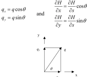
(2) hypothesis: the purely advective terms can be neglected. As a consequence the free surface slope is balanced by sole the friction term. 2.1 Physical system and conceptual model The SWE model simulates any steady or unsteady situation, possibly taking into consideration air transport or sediment-laden flows. The DM model is restricted to a specific range of Froude and kinematic numbers, but requires significantly less CPU resources. The large majority of flows occurring in rivers can reasonably be seen as shallow and characterized by relatively small vertical velocity components everywhere except in the vicinity of some singularities. This confirms the relevance of the SWE approach, which is in addition coupled to a turbulence model based on the Prandtl mixing length concept. The DM is more restrictive in the sense that it assumes the advective terms to be negligible in comparison with gravity and friction terms. The DM is preferred here only for steady flows. However these conditions are very widely met in waterways and the numerical results demonstrate the relevance of the approximation. The appropriateness of the assumptions must thus be recognized in view of practical applications presenting relatively moderate gradients, such as gradual floodings. The divergence form of the SWE include the mass balance:. ∂H ∂qi + =0 ∂t ∂xi. (1). and the momentum balance:  ∂qi ∂  qi q j    ∂H  +   = 0;    + gh  S fi + ∂t ∂xi  h   ∂xi   144 42444 3. j = 1, 2 , (2). inertia terms. where Einstein’s convention of summation over repeated subscripts has been used. H represents the free surface elevation, h is the water height, qi designates the specific discharge in direction i and Sfi is the friction slope. The diffusive assumption leads to a considerable simplification of the momentum equations:. S fi = −. ∂H ∂xi. (3). The general formulation of a friction law can be stated as a relation between the discharge, the water height and the slope: γ.  ∂H  q = αh S f = αh    ∂s  χ. γ. χ. (4). where α, γ and χ are coefficients suitable for the description of floodplain flows. Among others, Turner (Turner A. K. 1984) have provided a specific formulation for particular flows accross vegetation. The projection of the total discharge and of the free surface slope along the cartesian axes leads to:. qx = q cos θ q y = q sin θ. ∂H ∂H cos θ = ∂x ∂s ∂H ∂H sin θ = ∂y ∂s. and. (5). y. qy. q. θ qx. x. Figure 1 : Projection of the total discharge on the Cartesian axes.. As a consequence, the continuity equation (1) may be rewritten γ −1  ∂H ∂  χ ∂H ∂H cos θ  − α h  ∂t ∂x  ∂s ∂s  γ −1  ∂  ∂H ∂H − α hχ sin θ  = 0  ∂y  ∂s ∂s . (6). or γ −1 ∂H ∂  χ ∂H ∂H  − α h  ∂t ∂x  ∂s ∂x  γ −1 ∂  χ ∂H ∂H  − α h =0 ∂y  ∂s ∂y . (7). In short, equation (7) becomes: ∂H ∂  ∂H =  Dx ∂t ∂x  ∂x.  ∂  ∂H    +  Dy ∂y   ∂y . (8). where Dx and Dy act as nonlinear diffusion coefficients. 2.2 Algorithmic implementation 2.2.1 Space discretization A finite volume scheme is used in all models to ensure exact mass conservativity, which is a prerequisite for handling properly discontinuous solutions like moving hydraulic jumps. As a consequence no assumption is required regarding to the smoothness of the fields. Furthermore an automatic mesh re-.

(3) finement tool has been developed to boost the convergence rate towards highly accurate solutions. 2.2.2 Flux evaluation and boundary conditions In addition to the well-established Roe scheme, an original FVS is presented for space discretization of the complete set of equations (Mouzelard 2002). The stability of this second order upwind scheme has been demonstrated through a theoretical study of the mathematical system as well as a von Neumann stability analysis. Much care has been taken to handle correctly the source terms representing topography gradients. The models allow the user to specify any inflow discharge as an upstream boundary condition (BC). The downstream boundary condition can be a free surface elevation, a water height, a Froude number or even no specified condition if the outflow regime is supercritical (SWE only). 2.2.3 Matrix formulation of the DM A fully centered space discretization of the right hand side of equation can be performed thanks to the following relations : ∂  ∂H  ∂  ∂H    Dx  +  Dy ∂x  ∂x  ∂y  ∂y . H i , j +1 − H i , j 1   Dx , j + 1 ∆y  ∆y 2. hχ. 1 1 i+ , j i+ , j 2 2. H i , j − H i , j −1      −  Dx , j − 1  ∆y     2. G1 =. 1 1 D 1 , G2 = 2 D 1 2 ∆y x , j + 2 ∆y x , j − 2. H i +1, j − H i , j ∆x. 1 cos θ. 1 i+ , j 2. γ −1. D. 1 i− , j 2. =α. hχ. 1 1 i− , j i− , j 2 2. H i , j − H i −1, j ∆x. 1 cos θ. 1 i− , j 2. γ −1. D. 1 i, j + 2. =α. hχ. 1 1 i, j + i, j+ 2 2. H i , j +1 − H i , j ∆y. 1 sin θ. i, j+. 1 2. γ −1. D. 1 i, j − 2. =α. hχ. 1 1 i, j− i, j− 2 2. H i , j − H i , j −1 ∆y. − ( F1 + F2 + G1 + G2 ) H i , j = 0 1 1 D 1 , F2 = 2 D 1 2 ∆x x + 2 , j ∆x x − 2 , j. γ −1. =α. The relation above can be written in a better form for the later resolution:. F1 =. where. 1 i+ , j 2. (10).    . (9). D. H i +1, j − H i , j   H i , j − H i −1, j   1   Dx + 1 , j  −  Dx − 1 , j  + ∆x  ∆x ∆x     2 2 H i , j +1 − H i , j   H i , j − H i , j −1   1   Dx , j + 1  −  Dx , j − 1  = 0 ∆y  ∆y ∆y 2 2    . F1 H i +1, j + F2 H i −1, j + G1 H i , j +1 + G2 H i , j −1. H i +1, j − H i , j   H i , j − H i −1, j 1  ≈  Dx + 1 , j  −  Dx − 1 , j ∆x  ∆x ∆x   2 2 +. tion are intended to serve as fairly good initial condition for the complete SWE model. A first approach for solving the DM might be a pseudo-time evolution, starting from a user-defined initial condition. In order to prevail the possibility of using large time steps, this pseudo-time integration would need to be performed in an implicit way. A second approach is to disregard the time derivative term in (8) and to solve a non-linear system of time independent equations. Both methods are obviously very similar if the time step becomes very large. Consequently let’s consider the following system of equations:. 1 sin θ. i, j−. 1 2. The primary goal of this diffusive formulation is the quick computation of steady-state approximate solutions. Those first estimations of the final solu-. (11). More generally, this system of equations takes the form [ A][ H ] = [ R ] . Various iterative techniques are available for solving such very large linear systems. Among them are the methods « by point » (Jacobi, Gaus-Seidel,… (Hirsch 1990), (Young)) or full implicit (ADI (Kim and Douglas), (Malhotra, Douglas et al.), (Douglas and Kim 1999), (Molls and Zhao), (Panagiotopoulos and Soulis), GMRES (Saad and Schultz 1986)), CG (Jones and Plassman), (White), (Lin and J), (CACR)) 2.2.4 Iterative methods An implicit pseudo-time integration scheme, suitable for solving non-transient problems, is implemented in the SWE model. This technique allows to use much larger time steps than those acceptable for an explicit time integration. On the other hand the resolution procedure is more intricate. A Newton method is exploited to solve the large non-linear system. The successive linearized systems are solved with the powerful GMRES algorithm, which is advantageously coupled to a preconditioner. For this purpose an Incomplete LU decomposition is applied. The Switched Evolution-Relaxation technique by.

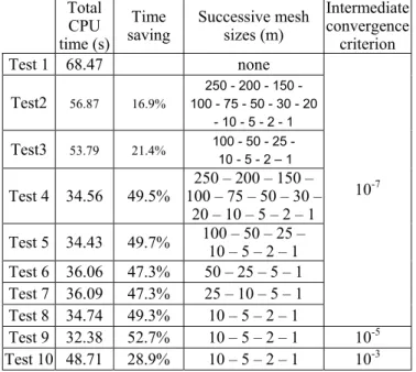
(4) Van Leer has been used to continuously optimise the time step (Van Leer 1982). In the DM model the GMRES or CG algorithms are also used for evaluating iteratively the solution of the symmetric linearized system. In both cases the resolution procedure represents a very challenging step because of the complexity of a cost-effective evaluation of the Jaobian matrix. WOLF performs this job effectively, by storing only non-zero elements and their location in the large sparse matrix (Saad 1996). 2.2.5 Mesh refinement On the basis of input data available on the finest grid, on which a steady-state solution is searched, computations are conducted on several successive grids, first very coarse and then gradually refined. The hydrodynamic fields are almost stabilized when the computer code automatically jumps onto the next grid. This entirely automatic method provides the advantage of drastically reducing the number of cells in the first grids. In case of an explicit pseudo-time evolution : the stable time step is significantly larger since it depends linearly on the size of the mesh. The successive so-called initial solutions are interpolated from the coarser towards the finer grid in terms of both water heights and discharges. For an implicit evolution, the benefits of the quadratic convergence are reached since the initial solution is sufficiently close to the stable solution. The drawbacks include the extra computation time to re-mesh and linearly interpolate the initial solution as well as the new boundary conditions. The optimal choice of convergence criterion for the intermediate solutions is also a critical point. In spite of these additional calculations necessary for generating the grid and for interpolating the initial solution or boundary conditions, the overall CPU time saving remains appealing. To illustrate this technique, several examples will be detailed in a subsequent paragraph of the paper. 2.2.6 Other features A fully objective calibration of friction coefficients is possible automatically with the WOLF’s optimisation tool, which is based on the innovative Genetic Algorithms (Erpicum 2001). 3 VALIDATION STUDIES This section contains a methodical assessment of the extent of the computation time reduction enabled by the DM and by the improvements brought to the SWE model. The section includes well illustrated comparisons of DM vs SWE, explicit vs implicit time integrations, fixed mesh vs automatic mesh re-. finement technique, … In the later case guidelines are given for choosing an optimal number of successive mesh refinements and for identifying appropriate criteria to switch from one grid to the next one. Moreover we describe case studies of inundation maps plotted for a natural river in Belgium, for which a high resolution Digital Elevation Model exists. Comparison with measurements and aerial photographs of recent major flood events will demonstrate the validity of the computer codes. CPU time requirements and achieved accuracy are compared for both numerical models. 3.1 Automatic mesh refinement 3.1.1 Water surface profile A first example to illustrate the potential time savings due to the mesh refinement technique is a simple 1D steady water profile. The characteristics of simulation are: channel length = 500 m; flat bottom; uniform friction coefficient K = 25 (International units), downstream level = 3 m; no-flow initially. The discharge imposed upstream is 5 m³/s and the finest mesh size is 1 m. Several tests were carried out in order to analyze the influence of various parameters of the automatic mesh refinement tool. The results are summarized in the table below (Table 1). Table 1: Description of the tests of mesh refinement carried out for a one-dimensional water profile. Total CPU time (s) Test 1 68.47. Time saving. Successive mesh sizes (m). Intermediate convergence criterion. none. Test2. 56.87. 16.9%. Test3. 53.79. 21.4%. Test 4. 34.56. Test 5. 34.43. Test 6 Test 7 Test 8 Test 9 Test 10. 36.06 36.09 34.74 32.38 48.71. 250 - 200 - 150 100 - 75 - 50 - 30 - 20 - 10 - 5 - 2 - 1 100 - 50 - 25 10 - 5 - 2 – 1. 250 – 200 – 150 – 49.5% 100 – 75 – 50 – 30 – 20 – 10 – 5 – 2 – 1 100 – 50 – 25 – 49.7% 10 – 5 – 2 – 1 47.3% 50 – 25 – 5 – 1 47.3% 25 – 10 – 5 – 1 49.3% 10 – 5 – 2 – 1 52.7% 10 – 5 – 2 – 1 28.9% 10 – 5 – 2 – 1. 10-7. 10-5 10-3. First of all, a reference computation was executed on a unique grid. Then, as a result of the onedimensional character of the present flow, the following intermediate grids are composed of rectangular cells in such a way that the width of the river is preserved. Consequently the time steps remains restricted by the smallest dimension of the meshes, i.e. the constant width. Consequently, in tests 2 and 3 the reduction of CPU time is not a result of larger.

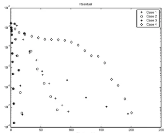
(5) time step. In the following tests, the time step has been continuously evaluated and optimized considering the specific flow conditions and mesh size. The last two tests show the influence of the convergence criterion on the intermediary solutions. The first tests, carried out without optimization of the time step clearly state that in this configuration, numerous intermediate grids have an adverse effect on the benefits obtained in CPU time. Indeed, the time step remaining strictly limited, the waves do not propagate fast enough on the very large cells. Alternatively, when the time step is suitably optimized, the saving in time CPU still increases very significantly. The time loss caused by an increased number of refinements becomes negligible here since stabilization on the very large cells intervenes in only a few steps. The majority of the computation time is thus consumed on the finer grids and very often during the last stage. According to table 1, the sizes of the successive cells for the same number of intermediate stages, appear not to affect strongly the final time saving. It is therefore useless to multiply the very coarse grids. The last tests carried out (8, 9 and 10) highlight the pointlessness of seeking a very high degree of accuracy on the intermediary results. Nevertheless, a too weak convergence of those penalizes the computing time. It can also be noticed that the additional benefit obtained is not very significant while the loss due to a bad convergence is very sensitive. In conclusion, the total saving of computation time is obvious. Although the choice of the number of intermediate steps doesn’t influence appreciably the final profit, an abusive multiplication of consecutive grids must be avoided. The intermediate convergence levels may be selected of one or two orders of magnitude higher than the desired final precision. 3.1.2 Curved open channel Another example dedicated to illustrate the mesh refinement technique is presented below. The steadystate hydrodynamic solution in a 90°-curved channel is considered. The discharge imposed upstream is 1 m³/s and the flume is 1 m wide. The downstream boundary condition is given by a free surface elevation of 1 m and the flow in the channel is initially at rest. The solution was with a fully implicit timeintegration scheme available in WOLF (Dewals 2002). Hence, this application also highlights that the technique is completely independent of the selected time integration scheme. The evolution of the residual as a function of the computation time is represented on Figure 3. In the first case, two successive grids are used. A first solution is obtained on a coarse grid with meshes of 40 cm. Then the final solution is reached on meshes of 10 cm.. (a). (b). Figure 2: Contour of the coarse grid (a) and solution at the first time step for specific discharge (m²/s). Stabilized solution on the finest grid of 10 cm (b).. Like previously mentioned, the swift decrease of the residual on the first grid is followed by an increase at the transition onto the finer grid. In spite of this increase of the residual, applying progressive refinement is justified by the substantial difference in the time CPU required to carry out one iteration on the coarse grid compared to the finer one. Residual. -2. 10. Case 1 Case 2 Case 3 Case 4. -3. 10. -4. 10. -5. 10. -6. 10. -7. 10. -8. 10. 0. 50. 100. 150. 200. 250. CPU time [s]. Figure 3: Evolution of the residual during the convergence towards a steady-state two-dimensional solution. In the second case, an additional mesh size has been used to investigate how far the advantages of refinement offset for the additional operations to change grid. Three different of meshes are considered: 40 cm, 20 cm and 10 cm. Figure 3 shows that this approach is proving to be even more competitive than the previous one. In the third case, the convergence criterion for the intermediate results has been reduced. The computation time has clearly increased because of a useless research of precision at the intermediate time steps. Finally, in the last case, calculation is performed immediately on the finest grid. This CPU time can be regarded as a reference to assess the benefits of the three previous strategies. 3.1.3 Large reservoir The last illustrative example covers the computation of a steady hydrodynamic situation in a large reservoir. This situation has immediate practical applica-.

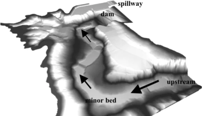
(6) tions such as the determination of a spillway rating curve or the assessment of silting risks behind the dam. The higher difficulty of this particular case is related to the total number of cells and to the complex natural topography involved. The size of the finest mesh is 3 m and the total surface of the domain is 2.25 km², requiring thus a total of up to 176.000 cells. The flood discharge considered is 10.000 m³/s. For the steady state computation is free surface is first supposed to be horizontal with zero velocity. The outflow at the spillway is supercritical and thus doesn’t call for any boundary condition.. piles near the spillway remain completely invisible on all the coarsest grids and are properly taken into account solely on the 3m-grid (see Figure 6). On the other hand the general flow distribution was already relevant on the first grid. The representation (Figure 7) of the residual decrease as a function of the total computation time clearly demonstrates the time-saving brought by automatic mesh refinement. At each change of grid, the time necessary to reach the same required accuracy (namely 2 10-3) increases by one order of magnitude.. spillway dam. Wakes of the piles. (b). (a) upstream. Figure 6: Zoom in the vicinity of the spillway, underlining the influence of the piles. (a) First iteration on the finest grid and (b) final stabilized solution.. minor bed. Figure 4: 3D view of the topography in the reservoir upstream of Kol Dam (India).. 1.E-01 Avec remaillage Sans remaillage. To converge towards the stabilized solution, five intermediate stages were completed: square meshes of respectively 48, 24, 12, 6 and 3 m. The evolution of the computation is represented on Figure 5.. 1.E-02. 1.E-03 1. 10. 100. 1000. 10000. 100000. Figure 7 : Evolution of the residual as a function of the CPU time, during the computation with four successive refinements () and without mesh refinement (). In the latter case the residual hardly doesn’t decrease.. Piles. This is easily comprehensible since the size of the cells is repeatedly divided by a factor 2. The total number of meshes is thus multiplied by 4 and the time-step divided by two according to the Courant stability criterion. As a result the computation length gets each time burdened with a factor as high as eight. 3.2 DM vs SWE. Figure 5 : Representation of the specific discharges (m²/s) stabilized on grids of 48, 24, 12 and 3 m respectively.. The shape of the domain is first roughly approximated and becomes better as the computation moves from one grid to the next. For instance the 12. In all test cases, the DM is more efficient to converge to a stationary solution than the SWE, even with a full implicit implementation. Nevertheless, fundamental differences can be observed due to neglected terms in the DM formulation. For instance, the water elevations computed with an usual roughness Manning coefficient of the river.

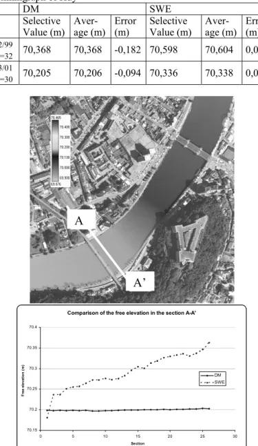
(7) Meuse applied to normal flows are underestimated, with the DM, at the limnigraph of Huy. This one is located on the right bank after a marked meander and a bridge with two piers in the main river bed. The below representation (Figure 8) of the water elevation in a cross-section at the level of the limnigraph shows that the solution of the DM is near horizontal in absence of inertial terms. The SWE increases naturally this slope. As result, a difference of about 10 cm appears between the two banks and the resulting error at the comparison point becomes small. Consequently, the modeler must pay attention to the location of the validation points. An inadequacy of them with the used model can lead to substantial errors on the final solution.. dams of Andenne-Seilles and Ampsin-Neuville. The developed length is about 15 km. Multiple recurring flood areas can be observed during real events, notably the floods of 1993 and 1995. The topographic data of floodplains and bathymetric data of the main river bed are obtained from the Ministry of Equipment and Transports, Belgium (SETHY). The spatial resolution is one point per square meter and the vertical accuracy is 15 cm. The discharge is 2159 m³/s. The downstream water height if fixed by the limnigraph of Ampsin. The total number of computed cells is about 650,000.. Table 2: Water elevations and errors of the DM and SWE at the limnigraph of Huy DM SWE Selective AverError Selective AverError Value (m) age (m) (m) Value (m) age (m) (m) 12/99 K=32 03/01 K=30. 70,368. 70,368. -0,182 70,598. 70,604. 0,049. 70,205. 70,206. -0,094 70,336. 70,338. 0,038. A. A’ Comparison of the free elevation in the section A-A' 70.4. Free elevation (m). 70.35. 70.3. DM SWE 70.25. 70.2. 70.15 0. 5. 10. 15. 20. 25. 30. Section. Figure 8 Comparison of the water elevation at the cross section A-A’. 3.3 Inundation risk and flood extension The reach of Meuse considered is the same as the previous example and is located between the mobile. Figure 9 Example of mesh refinement for the determination of the flood extension along the river Meuse (Belgium)..

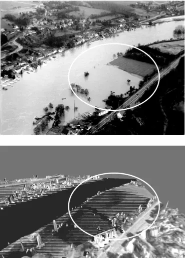
(8) The above representations (Figs. 9) illustrate the progressive refinement of the meshes (40, 20, 10 and 5 m) and the determination of the flood extension. It can be observed that some areas, inundated on a large grid, can dry as consequence of a refinement of the topographic elevation (e.g. a road creating an artificial obstruction of the floodplain). Figure 10 illustrates the good correspondence of the flood extension between the real event and the simulation.. Figure 10 Comparison of numerical results with an aerial photography of a flood event (Belgium).. As a final result, the fields of water heights and discharges obtained from the simulation can be combined with a map of ground occupancy to determine a global risk map. 4 CONCLUSION In conclusion the paper comprehensively outlines advantages and drawbacks of both numerical models, studied in the very practical view of investigating floodplains and inundation maps. It constitutes thus a genuine bridge linking highly sophisticated considerations in applied mathematics with major concerns of practitioners and decision makers in the field of flood control (state agencies, insurance and reinsurance companies…). Perspectives of im-. provements in the near future include the analysis of sediment transport effects and their modelling. 5 REFERENCES Archambeau, P., B. Dewals, et al. (2001). "De l'utilité de la modélisation numérique en hydrodynamique de surface." Ingenieurbiologie / Génie biologique 4: 9-20. CACR, C. f. a. c. r. (2000). NAG Libraries. Dewals, B. J. (2002). Développement de modèles hydrosédimentaire pour la gestion de grands ouvrages hydrauliques, University of Liege. Douglas, J. and S. Kim (1999). On accuracy of alternating direction implicit methods for parabolic equations. 2002. Dworak, T., W. Hansen, et al. (2003). Workshop Report. International Workshop on Precautionary Flood Protection in Europe, Bonn, Germany, Ecologic. Erpicum, S. (2001). Application des algorithmes génétiques aux problèmes d'optimisation en hydrodynamique de surface, University of Liege. Hirsch, C. (1990). Numerical Computation of Internal and External Flows, Computational Methods for Inviscid and Viscous Flows, Wiley. Jones, M. and P. Plassman (1991). An improved incomplete Cholesky factorization. Illinois, Mathematics and Computer Science Division, Argonne National Laboratory: 12. Kim, S. and J. Douglas Fractional time-stepping methods for unsteady flow problems. Lin, C.-J. and M. J (1997). Incomplete Cholesky factorizations with limited memory. Malhotra, S., C. Douglas, et al. (2000). Parameter choices for ADI-like methods on parallel computers. Molls, T. and G. Zhao (2000). "Depth-averaged simulations of supercritical flow in channel with wavy sidewall." Journal of Hydraulic Engeneering 126(6): 437-445. Mouzelard, T. (2002). Contribution à la modélisation des écoulements quasi tridimensionnels instationnaires à surface libre. Département d'Hydraulique et de Transport, Université de Liège. Panagiotopoulos, A. and J. Soulis (2000). "Implicit bidiagonal scheme for depth-averaged free-surface flow equations." Journal of Hydraulic Engeneering 126(6): 425-436. Pirotton, M. (1994). Modélisation des discontinuités en écoulement instationnaire à surface libre. Du ruissellement hydrologique en fine lame à la propagation d'ondes consécutives aux ruptures de barrages, Université de Liège. Saad, Y. (1996). SPARSKIT: a basic tool-kit for sparse matrix computations. Minneapolis, University of Minnesota. Saad, Y. and M. Schultz (1986). "GMRES : A generalized minimal residual algorithm for solving non-symmetric linear system." SIAM Journal of Scientific and Statistical Computing 7. SETHY Service d'Etudes Hydrologiques du Ministère de l'Equipement et des Transports (MET), Belgium. Turner A. K., C. N. (1984). "Shallow flow of water trough nonsubmerged vegetation." Agricultural Water Management 8: 375-385. Van Leer, B. (1982). "Flux-Vector Splitting for the Euler Equations." Lecture Notes in Physics 170: 507-512. White, D. (1998). "Solution of Capacitance systems using incomplete Cholesky fixed point iteration." Journal for Numerical Methods in Engeneering. Young, D. M. (1971). Iterative solution of large linear system. New York, Academic Press..

(9)