TH`
ESE
En vue de l’obtention du
DOCTORAT DE L’UNIVERSIT´
E DE TOULOUSE
D´
elivr´
e par l’Universit´
e Toulouse III - Paul Sabatier
Discipline ou sp´
ecialit´
e :
Informatique
Pr´
esent´
ee et soutenue par
Anthony Pajot
Le 26 avril 2012
Toward robust and efficient
physically-based rendering
JURY
Rapporteurs :
Kadi Bouatouch, Pr., Universit´
e de Rennes 1
Nicolas Holzschuch, DR, INRIA Rhˆ
one-Alpes
Examinateurs :
George Drettakis, DR, INRIA Sophia-Antipolis
Xavier Granier, CR, INRIA Bordeaux Sud-Ouest
Invit´
e :
Pierre Poulin, Pr., Universit´
e de Montr´
eal
Ecole doctorale : Math´ematiques Informatique T´el´ecommunications de Toulouse
Acknowledgments
`
A la question “jusqu’`a quelle longueur c¸a peut faire, la section remerciements ?”, mon directeur de th`ese m’a r´epondu “pas plus long que la th`ese en elle-mˆeme !”.
Eh ben je peux vous dire que c’est court, parce que des remerciements, il y en a `a faire ! Et des sinc`eres hein, pas des remerciements dans le vent pour faire joli et parce que lorsque nous ´etions enfants on nous a dit d’ˆetre polis.
D´ej`a, je voudrais remercier ceux dont j’ai ´et´e le moins proche, mais qui ont eu un rˆole essentiel : les personnes qui ont jug´e mon travail. Rendez-vous compte : trois semaines avant la soutenance, un pav´e de 240 pages qui arrive avec peu d’images et limite plus d’´equations que de phrases. Et en plus ils ont dˆu se lever `a pas d’heure et traverser la France pour venir assister `a une pr´esentation. Et le pire de tout ca, ils n’ont presque pas pu profiter du pot de th`ese, leurs avions partant juste apr`es. Franchement, `a leur place, j’aurais dit non. Donc merci beaucoup `a vous pour le temps consacr´e `a l’examen de mon travail ! J’´ecris cette section presque un an apr`es la soutenance (des...euh...j’´etais tr`es occup´e, voyez-vous), et malgr´e ce petit laps de temps, les gens que j’ai pu rencontrer pendant les 3 ans et demi de la th`ese et ce qu’ils m’ont apport´e reste toujours aussi fort.
Il y a ceux dont c’est le m´etier, mais qui l’ont toujours fait pour tout autre chose que par pur profes-sionnalisme ou parce que c’est leur rˆole : mes encadrants, Mathias et Lo¨ıc. Pendant 3 ans et quelques, ils ont support´e mon opiniˆatret´e, ma mauvaise foi et mon sens inn´e de l’exag´eration. Et en plus de ca, Mathias a accept´e que je ne capte pas grand chose au d´ebut de ma th`ese et que je change de voie, Lo¨ıc a accept´e qu’il ne comprenne pas grand chose au d´ebut de ma th`ese (et mˆeme apr`es), et malgr´e cela est toujours revenu `a l’attaque, parce que bon, Monte-Carlo ca ne pouvait pas ˆetre QUE du bruit malgr´e ce que je lui montrais ! Bon, `a un moment ils en ont dˆu en avoir marre, parce qu’ils m’ont envoy´e pendant 3 mois `a l’autre bout du monde, chez un pauvre Montr´ealais qui avait pass´e 6 mois charg´es de bi...boissons `a bulle et de VTT `a Toulouse, et qui m’a acceuilli de la mani`ere la plus gentille du monde. Pierre, vous autres qu´eb´ecois vous ne savez peut-ˆetre pas faire du bon pain pantoute, mais ostie de criss qu’est-ce-que c’´etait bien ces trois mois de sauna..euh, d’´et´e `a Montr´eal dans ton lab ! Et qu’est-ce-que j’´etais content que tu viennes `a ma soutenance ! Apr`es mon retour, certainement parce que je n’avais pas chang´e, mes encadrants ont pris une troisi`eme personne pour mieux tenir le choc, David. Le pauvre ! Et `a cˆot´e de ca, VTT, montagne, Magic, tout ´etait pretexte `a discuter (ou `a me faire cracher mes poumons ou mes points de vie) dans une ambiance l´eg`ere, d´econtract´ee, mais o`u le travail avanc¸ait et les cerveaux fumaient gaiement !
Apr`es, il y a ceux qui m’ont soutenu sans raison particuli`ere. Ma famille par exemple. Toujours l`a quand j’en avais besoin mˆeme si je ne le disais pas. Toujours prˆets, un support pr´esent mais qui ne s’impose pas. Papa, Maman, Laurence et Arnaud, merci, vous avez ´et´e parfaits !
Et apr`es il y a les amis. Oulala, je vais rester bref (mais si mais si, je suis bref l`a), mais ca pourrait ˆetre long...
D´ej`a, il y a les personnes qui travaillaient dans la mˆeme salle que moi, ceux des salles d’`a-cˆot´e avec qui on allait manger... Et au del`a de c¸a, les moments partag´es en dehors de ce cadre ! Trois semaines
feuille de temps affich´ee dans la salle avec les meilleurs temps surlign´es et Samir qui voit ses “poulains” commencer s´erieusement `a revenir sur lui ? Et les parties de Magic endiabl´ees pendant les rares et tr`es courtes pauses que l’on faisait tous les jours entre 16h et 18h ? Le cours de physique au milieu des vaches (litt´eralement) `a Roffiac ? Les panneaux “help” pendant l’´enonc´e de l’exercice “bˆateau” du puit de potentiel quantique ? Les discussions sur tout et n’importe quoi les midis (notamment celles sur “pourquoi on repeindrait pas la salle en rose ?” qui rencontra une vive opposition) ? Les spectacles d’impros ? Etc. etc. En fait, toutes ces choses qui font que mˆeme si la th`ese en elle-mˆeme ne va pas, que ca avance pas, que ca rame, que ca en est d´esesp´erant, ben on va au labo avec la banane et une ´energie `a chaque fois renouvell´ee ! Donc un grand, un immense merci `a tous ceux qui ont rendu ces moments si savoureux, je suis ravi de vous cotˆoyer ou de vous avoir cotˆoy´es : Andra, Dorian, Franc¸ois, Guillaume, Jonathan, Laure, Marie, Mathieu G., Mathieu M., Nelly, Marion, Monia, Olivier, Philippe, Pignouf, Rodolphe, Roman, Samir, Sylvain, Shaouki, Vincent, et ceux dont j’aurais pu oublier le pr´enom !
Puis il y a les amis d’avant la th`ese aussi, Antoine, Benoit, C´edric, Julien, Lucas, et les amis d’encore avant, Lorraine et Ronan, qui m’ont fait rencontrer une bande de fous-furieux adorables `a Montr´eal ! D´ecarie, vraiment, c’´etait super cool !
Et puis il y a d’autres rencontres et d’autres moments, telles que les semaines `a Roffiac ou `a Odeillo avec les physiciens du Laplace, merci Richard et St´ephane de nous avoir donn´e cette opportunit´e. Vrai-ment, les vaches qui regardent le tableau rempli d’´equations, c’´etait un grand moment !
Et enfin, il y a aussi les personnes rencontr´ees en dehors de la th`ese, qui sans le savoir vous font oublier les tracas, et dont certains deviennent des amis. Benoit, Carine, Laurent et tous les fadas montag-nards, merci pour tous ces bons moments pass´es en montagne ou ailleurs, qui permettaient de revenir le lundi matin avec le sourire jusqu’aux oreilles ! Et vivement les prochains ! Et merci aux gens des clubs d’impro et de sport que j’ai cotˆoy´e durant cette p´eriode et que je continue `a cotˆoyer avec joie !
Pour r´esumer, merci `a toutes les personnes que j’ai crois´e durant cette p´eriode, et qui directement ou indirectement, m’ont permis de relever ce d´efi !
`
Contents
Partie I Introduction 1
Version franc¸aise 3
English version 7
Partie II Context 11
Chapter 1 Physical modelisation of light transport for rendering 13
1.1 Image, pixel, rendering process . . . 13
1.2 Radiometry . . . 14
1.2.1 From spectral radiance to energy: radiometric integrals . . . 15
1.2.2 From energy to spectral radiance: differential formulation . . . 17
1.2.3 Relation between incident and outgoing quantities . . . 18
1.2.4 Spectral distributions . . . 19
1.3 Colorimetry . . . 19
1.3.1 Chromaticity, luminance, gamut . . . 20
1.3.2 RGB, gamma correction, white point, sRGB . . . 20
1.4 From radiometry to colorimetry . . . 22
1.4.1 Spectrum → RGB conversion . . . 24
1.4.2 Spectrum → CIE XYZ → RGB . . . 24
1.5 Content of a HDR image, sensor . . . 26
1.5.1 Reconstruction filter . . . 27
1.5.2 Signal value, sensor response . . . 27
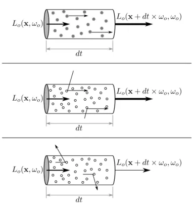
1.6 Light interactions . . . 28
1.6.1 Self-emission . . . 28
1.6.2 Absorption and scattering . . . 29
1.7.1 Absorption and scattering at surfaces . . . 31
1.7.2 Absorption and scattering in participating media . . . 34
1.8 Light transport equations . . . 39
1.8.1 Light transport in empty space . . . 39
1.8.2 Light transport with participating media . . . 39
1.9 Summary and final equations . . . 41
1.9.1 Hypotheses . . . 41
1.9.2 Spectral rendering . . . 42
1.9.3 Color-space rendering . . . 42
1.9.4 Final equations . . . 44
1.10 Conclusion . . . 45
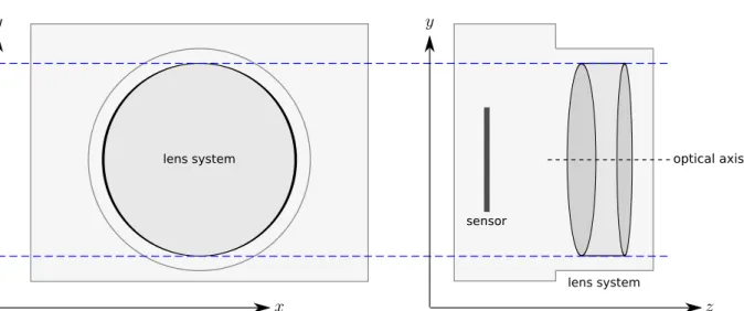
Chapter 2 Description of a scene for physically-based rendering 47 2.1 Camera model . . . 47
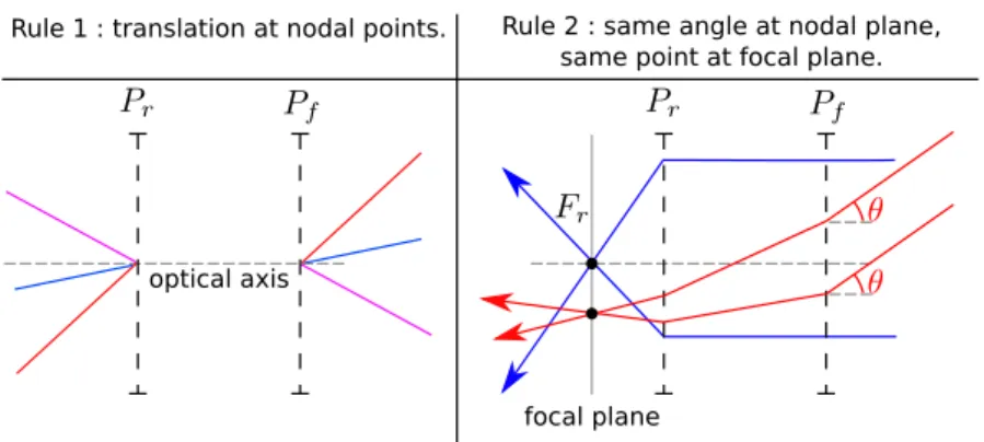
2.1.1 Optical model of lens systems . . . 48
2.1.2 Putting lens systems and sensors together . . . 51
2.1.3 Radiometric model . . . 54
2.2 Light sources . . . 55
2.2.1 Local light sources . . . 55
2.2.2 Distant light sources . . . 55
2.3 Geometry . . . 56
2.3.1 Geometry representation . . . 56
2.3.2 Efficient ray-tracing function . . . 59
2.4 Materials . . . 61
2.5 Participating media . . . 62
2.6 Conclusion . . . 62
Chapter 3 Mathematical tools for physically-based rendering 63 3.1 Path-integral formulation . . . 63
3.1.1 Path representation and light sources types . . . 64
3.1.2 Path space, path space measure . . . 64
3.1.3 Rpand f . . . 66
3.2 Tools for numerical integration . . . 67
3.3 Probability to have a section on probabilities = 1 . . . 67
3.3.1 Random variable . . . 67
3.3.2 Probability density function, cumulative density function . . . 69
3.3.4 Equivalence of random variables, i.i.d. random variables, impact of PRNGs
on independence . . . 72
3.3.5 Function of random variable(s), expected value . . . 72
3.4 Estimators, standard Monte-Carlo estimator . . . 73
3.4.1 Bias, variance, robustness . . . 74
3.4.2 Dirac-delta distributions and Monte-Carlo . . . 77
3.5 Variance reduction methods . . . 79
3.5.1 Importance sampling . . . 79
3.5.2 Multiple importance sampling . . . 80
3.5.3 Control variate . . . 81
3.5.4 Uniform samples placement . . . 81
3.6 Non-standard Monte-Carlo methods . . . 83
3.7 Sampling optical paths . . . 84
3.7.1 Local importance sampling of optical paths . . . 84
3.7.2 Russian roulette . . . 86
3.8 Conclusion . . . 86
Partie III Contributions 89 Chapter 4 A versatile software architecture for physically-based rendering 91 4.1 From equations to software architecture . . . 92
4.1.1 Image reconstruction and processing . . . 93
4.1.2 Physical simulation . . . 94
4.1.3 Rendering control . . . 97
4.2 Examples of components . . . 97
4.2.1 Integrator . . . 97
4.2.2 Simulator . . . 101
4.2.3 Adaptive screen sampling . . . 102
4.2.4 Accumulator . . . 103
4.2.5 HDR processor . . . 103
4.3 Robust and efficient rendering . . . 104
Chapter 5 Representativity for robust and adaptive multiple importance sampling 107 5.1 Introduction . . . 107
5.2 Related works . . . 110
5.2.1 Importance sampling strategies for rendering . . . 110
5.3 Variance-optimal sampling configurations . . . 112
5.4 Representativity-based sampling . . . 113
5.4.1 BSDF-based strategy representativity . . . 114
5.4.2 Photon-map-based strategy representativity . . . 115
5.4.3 Sampling configurations from representativities . . . 118
5.4.4 General hints for defining representativities . . . 119
5.5 Numerical analyses . . . 120
5.5.1 Simple scenes . . . 121
5.5.2 Chains of estimators . . . 126
5.6 Examples of applications . . . 131
5.6.1 Photon mapping final gathering . . . 131
5.6.2 Photon-map guided path-tracing . . . 131
5.6.3 Direct lighting in highly occluded environment . . . 131
5.6.4 Other contexts than MIS-based estimation . . . 131
5.7 Conclusion . . . 132
Chapter 6 Sample-space bright spots removal using density estimation 133 6.1 Introduction . . . 133
6.2 Related works . . . 135
6.2.1 Image-space bright spots removal . . . 135
6.2.2 Sample-space bright spots removal . . . 136
6.2.3 Outlier detection . . . 136
6.3 Bright-spot removal using density estimation . . . 137
6.3.1 Adaptive bandwidth . . . 139
6.4 Lowering memory consumption . . . 140
6.4.1 Algorithm overview . . . 140
6.4.2 Approximate distribution representation (ADR) . . . 141
6.4.3 ADR: analysis . . . 142
6.4.4 Rule-of-thumb bandwidth (ROT) . . . 143
6.4.5 ROT: analysis . . . 143
6.4.6 Switching from ADR to ROT . . . 144
6.5 Results . . . 146
6.6 Conclusion . . . 148
Chapter 7 Effective despeckling of HDR images 151 7.1 Introduction . . . 151
7.3 Results . . . 153
7.4 Conclusion . . . 158
Chapter 8 Robust adaptive screen-sampling for Monte-Carlo-based rendering 159 8.1 Introduction . . . 159
8.2 Robust error-based adaptive sampling . . . 160
8.3 Results . . . 162
8.3.1 Robustness to outliers . . . 162
8.3.2 Adaptive sampling evaluation . . . 163
8.4 Conclusion . . . 165
Chapter 9 Globally adaptive control variate for least-square kd-trees on volumes 169 9.1 Introduction . . . 169
9.2 Related works . . . 170
9.2.1 Participating media representations . . . 170
9.2.2 Numerical integration . . . 171
9.3 Error-guided kd-tree . . . 173
9.3.1 Error measure . . . 174
9.3.2 Cost minimization . . . 175
9.3.3 Enforcing global error from local errors . . . 176
9.3.4 Generalization . . . 176
9.4 Globally adaptive control variate . . . 177
9.4.1 Overview . . . 177
9.4.2 Estimations . . . 179
9.4.3 Convergence criterion . . . 180
9.4.4 Kd-tree as control variate . . . 180
9.4.5 Control variate and estimations interactions . . . 182
9.4.6 Estimation error . . . 182
9.4.7 Integrals over arbitrary finite-dimensional supports . . . 183
9.5 Results . . . 184
9.5.1 Numerical integration . . . 184
9.5.2 Trees . . . 190
9.6 Extensions . . . 194
9.7 Conclusion . . . 195
Chapter 10 Combinatorial bidirectional path-tracing for efficient hybrid CPU/GPU ren-dering 197 10.1 Introduction . . . 197
10.2 Related works . . . 198
10.3 Combinatorial bidirectional path-tracing (CBPT) . . . 198
10.3.1 Base algorithm . . . 198
10.3.2 Discussion . . . 201
10.4 Efficient computation of combination data . . . 202
10.5 Implementation of CBPT . . . 204
10.6 Results . . . 205
10.6.1 Combination throughput . . . 207
10.6.2 CBPT . . . 208
10.7 Conclusion . . . 212
Partie IV Final summary and conclusions 213
Bibliography 219
Part I
Version franc¸aise
L’informatique graphique est utilis´ee dans des domaines nombreux et vari´es. Les besoins en r´ealisme et en complexit´e visuelle pr´esent´es pour le divertissement augmentent tr`es rapidement, que ce soit les ef-fets sp´eciaux dans les films, les environnements des jeux vid´eos ou mˆeme les publicit´es. L’informatique graphique devient aussi un moyen d’aide `a la d´ecision : la pr´evisualisation virtuelle d’objets ou de bˆatiments permet aux designers et architectes de prendre en compte des aspects visuels difficiles `a se repr´esenter mentalement, tels que l’influence de l’´eclairage sur la perception d’une pi`ece. De mˆeme, les illustrations sont un moyen efficace pour mieux appr´ehender des id´ees complexes ou des concepts ab-straits, ou tout simplement garder l’attention de l’auditoire. Que ce soit pour le divertissement ou l’aide, l’informatique graphique peut endosser plusieurs fonctions : d´emonstration, remplacement d’objets dif-ficiles `a construire par des maquettes virtuelles, simulation, ou bien encore visualisation de mondes virtuels. Pour chacune de ces fonctions, il existe des types de pr´esentations qui r´epondent plus ou moins bien aux besoins : le rendu non-photor´ealiste est adapt´e pour les sch´emas, les plans ou bien encore les illustrations, grˆace `a la grande libert´e existante dans les styles graphiques utilisables. Ceci dit, mˆeme quand le photo-r´ealisme est d´esirable, un large panel de possibilit´es est disponible, en fonction des con-traintes qui sont pos´ees : un faible coˆut de calcul pour les jeux, un haut niveau de contrˆole artistique pour les films, une grande pr´ecision au prix de calculs tr`es coˆuteux dans le cadre du rendu pr´edictif (rendu dit physiquement r´ealiste), ou bien encore des coˆuts de calcul moindres via l’utilisation d’approximations dont l’impact est connu comme ´etant mineur pour les sc`enes trait´ees (rendu dit bas´e sur la physique).
Dans cette th`ese, nous nous concentrons sur ce dernier type de rendu : nous visons le photo-r´ealisme,
sans n´ecessiter de trucages de la part d’un cr´eateur de contenu pour reproduire un effet d’´eclairage
particulier, dans un nombre de sc`enes aussi grand que possible, i.e. des sc`enes o`u les approximations faites ont un impact imperceptible. Pour cela, il est n´ecessaire de simuler le comportement de la lumi`ere, en choisissant consciencieusement les approximations faites, afin de pouvoir traiter un maximum de sc`enes d’une mani`ere qui soit proche du comportement r´eel de la lumi`ere.
Les ´equations utilis´ees pour la simulation, que l’on d´erive au Chapitre 1, prennent en compte le comportement de la lumi`ere tel que d´ecrit par la physique, ainsi que la mani`ere dont une image peut ˆetre calcul´ee `a partir de cette mod´elisation, en incluant les ph´enom`enes de perception humaine. La physique de la lumi`ere est bas´ee sur une mod´elisation macroscopique, d´ecrite par la radiom´etrie, et sur des ´equations dites de transport lumineux. Ces ´equations font partie du domaine du transfert radiatif. Pendant la d´erivation, nous montrons que prendre en compte tous les ph´enom`enes lumineux, mˆeme en se limitant aux ph´enom`enes macroscopiques d´ecrivables par la radiom´etrie, implique entre autre une
extrˆeme complexit´e et des temps de calculs prohibitifs. Nous explicitons donc les approximations qui sont couramment faites dans le cadre du rendu bas´e sur la physique. Ces ´equations nous permettent de calculer une image telle que vue par une cam´era plac´ee dans une sc`ene comprenant des sources de lumi`eres, des objets et des milieux continus tels que la fum´ee ou le brouillard. Ces entit´es doivent ˆetre d´ecrites et repr´esent´ees dans un formalisme compatible avec la simulation. Une br`eve revue de ces repr´esentations est effectu´ee dans le Chapitre 2. Les ´equations qui doivent ˆetre r´esolues durant la simula-tion sont des int´egrales, qui ne peuvent ˆetre calcul´ees de mani`ere analytique pour des sc`enes arbitraires. Des m´ethodes num´eriques doivent donc ˆetre employ´ees. Bien que plusieurs approches existent, nous nous concentrons dans cette th`ese `a la m´ethode la plus couramment utilis´ee actuellement en rendu bas´e sur la physique, `a savoir la m´ethode de Monte-Carlo, que nous pr´esentons dans le Chapitre 3.
Utiliser ces outils math´ematiques pour effectuer la simulation physique dans le cadre du rendu re-quiert une architecture logicielle adapt´ee. Notre premi`ere contribution, expos´ee dans le Chapitre 4, est une architecture logicielle inspir´ee de celle de moteurs de rendu connus, mais ayant une flexibilit´e ac-crue. Cette architecture est bas´ee sur une d´ecomposition fonctionnelle des ´equations de la physique, en prenant en compte la nature des algorithmes li´es `a la m´ethode de Monte-Carlo, ainsi que les algorithmes d´evelopp´es dans le domaine du rendu. Nous montrons qu’un grand nombre d’algorithmes faisant partie de l’´etat de l’art et touchant `a divers aspects du rendu sont facilement implantables dans l’architecture que nous d´efinissons.
Le cœur d’un moteur de rendu bas´e sur la m´ethode de Monte-Carlo est la partie li´ee `a l’int´egration num´erique des ´equations du rendu, ´etant responsable de la simulation du transport de la lumi`ere. De mani`ere superficielle, faire du rendu avec la m´ethode de Monte-Carlo consiste `a utiliser quelques “ex-emples” (appel´es ´echantillons) de chemins que la lumi`ere peut suivre dans une sc`ene avant d’atteindre la cam´era, et d’en extrapoler la valeur qui serait obtenue si tous les chemins ´etaient pris en compte.
`
A notre connaissance, aucun algorithme de l’´etat de l’art ne peut traiter toutes les sc`enes possibles de mani`ere rapide et pr´ecise : pour chacun de ces algorithmes, il existe des sc`enes o`u l’algorithme donne de mauvais r´esultats, ou n´ecessite des temps de calculs trop importants. Cette sensibilit´e est un manque de robustesse, qui se traduit par des temps de calcul qui ne sont pas consistants. Pour chaque algorithme, les raisons pour lesquelles il n’arrive pas `a traiter telle ou telle sc`ene sont souvent techniques, et inconnues des utilisateurs principaux du moteur, `a savoir les artistes. De leur point de vue, ils sont donc confront´es `a des temps de calcul qui ne varient pas qu’en fonction de la complexit´e globale de la sc`ene, mais peuvent aussi devenir extrˆemement longs pour des configurations qui leur semblent arbitraires et impr´evisibles.
Plutˆot que de s’attaquer `a la d´efinition d’une m´ethode de simulation compl`etement robuste, nous choisissons dans cette th`ese de d´evelopper un ensemble de m´ethodes nous permettant d’am´eliorer la robustesse du processus de rendu global : nous d´eveloppons donc des m´ethodes ciblant plusieurs parties fonctionnelles d’un moteur de rendu. Plus pr´ecis´ement, nous avons d´evelopp´e des m´ethodes am´eliorant la robustesse de cinq parties d’un moteur :
• Int´egration : le choix des chemins a un fort impact sur la robustesse d’un moteur utilisant la m´ethode de Monte-Carlo, et ce quel que soit l’algorithme pr´ecis utilis´e pour la simulation. Dans le Chapitre 5, nous montrons comment am´eliorer la robustesse d’un grand nombre d’algorithmes
de simulation li´es au rendu, tout en n’introduisant qu’un faible surcoˆut en temps de calcul. • Reconstruction de l’image : en r´esum´e, l’image finale est obtenue en moyennant l’´energie qui
contribue `a chaque pixel. Quand la m´ethode d’int´egration, qui calcule cette ´energie `a partir d’´echantillons, n’est pas parfaitement robuste, quelques valeurs d’´energie peuvent ˆetre tr`es sup´erieure `a la valeur exacte du pixel, donnant des pixels isol´es tr`es brillants (points brillants). Ce probl`eme est dˆu au fait que rajouter ne serait-ce qu’une valeur tr`es grande `a un calcul de moyenne donne une sur-estimation tr`es marqu´ee de cette moyenne. Ces valeurs anormalement hautes sont appel´ees valeurs aberrantes. Le probl`eme des points brillants peut donc ˆetre vu comme une cons´equence du manque de robustesse de l’estimateur de la moyenne aux valeurs aberrantes. Dans le Chapitre 6, nous am´eliorons la robustesse de cet estimateur aux valeurs aberrantes en les d´etectant et en ne les ajoutant pas au calcul de la moyenne.
• Traitement d’images : les images calcul´ees par un moteur de rendu sont trait´ees avant d’ˆetre af-fich´ees, premi`erement pour qu’elles soient utilisables sans perte d’information sur un ´ecran ou une imprimante (cette op´eration est appel´ee correction de tons). Ces traitements peuvent ˆetre bas´ees sur des m´ethodes non-robustes, telle que diviser la valeur de tous les pixels par la valeur maxi-male sur les pixels. Cette m´ethode, ainsi que toutes celles bas´ees sur du filtrage non robuste (qu’il soit Gaussien ou pas), donnera de mauvais r´esultats d`es que des points brillants seront pr´esents. Comme d´ej`a dit ci-dessus, ces points brillants peuvent ˆetre caus´es par le fait que les m´ethodes d’int´egration et de reconstruction d’images ne sont pas parfaitement robustes, mais ils doivent ˆetre trait´es avant l’application d’une quelconque m´ethode de traitement d’images. Nous pr´esentons donc au Chapitre 7 une m´ethode pour recalculer la valeur des pixels ´etant des points brillants `a partir des pixels avoisinants, ´evitant ainsi la pr´esence de points brillants lors des diff´erents traite-ments effectu´es par la suite sur l’image.
• Choisir les pixels pour lesquels des ´echantillons sont calcul´es : comme chaque ´echantillon ne contribue qu’`a quelques pixels, ne devont choisir ces ´echantillons – et donc les pixels o`u les ajouter – de mani`ere `a ce que l’image soit aussi proche que possible d’une image “parfaite”, en concentrant les ´echantillons l`a o`u l’erreur est la plus grande. Ceci est appel´e de l’´echantillonnage adaptif, et la majorit´e des m´ethodes d’´echantillonnage adaptatif souffre d’un probl`eme d’“arrˆet pr´ematur´e” : un pixel pour lequel l’erreur est trouv´e faible une fois n’est jamais reconsid´er´e. Nous montrons dans le Chapitre 8 que ceci peut amener `a des artefacts tr`es visibles sur l’image, et donc `a un manque de robustesse, ind´ependamment de la robustesse des m´ethodes utilis´ees dans les autres parties fonctionnelles du moteur. Nous montrons une solution extrˆemement simple `a ce probl`eme, qui peut de plus ˆetre appliqu´ee `a toute m´ethode d’´echantillonnage adaptatif. De plus, nous montrons des moyens simples pour estimer correctement l’erreur d’un pixel mˆeme en pr´esence de valeurs aberrantes, et comment r´eduire l’erreur aussi bien dans les zones ombrag´ees que dans les zones fortement ´eclair´ees.
• Stabilit´e des temps de calcul : mˆeme si des m´ethodes robustes sont utilis´ees pour toutes les par-ties fonctionnelles d’un moteur de rendu, la description de la sc`ene doit aussi ˆetre ad´equate, afin
d’assurer une stabilit´e globale de l’ensemble du moteur de rendu. Dans le cas particulier des milieux participants, leur repr´esentation peut avoir un impact non-n´eligeable sur les temps de calcul : certaines sc`enes requi`erent dix ou cent fois plus de temps `a calculer que d’autres, unique-ment parce que les repr´esentations des milieux participants ne sont pas adapt´ees aux op´erations n´ecessaires pour faire du rendu bas´e sur la physique. Nous pr´esentons donc dans le Chapitre 9 une repr´esentation unifi´ee, qui peut ˆetre obtenue depuis n’importe quelle autre repr´esentation, et qui assure des temps de calculs faibles et stables mˆeme pour des milieux complexes. Cette con-tribution requi´erant une m´ethode d’int´egration num´erique extrˆemement robuste et efficace, nous d´eveloppons et pr´esentons une telle m´ethode, qui peut ˆetre utilis´ee dans de nombreux cadres autres que celui de l’approximation des milieux participants.
Enfin, un moteur robuste qui soit ´egalement efficace serait tr`es avantageux : les temps de calcul seraient ainsi stables et faibles pour un nombre tr`es important de sc`enes. Afin de tendre vers cela, nous proposons comme derni`ere contribution dans le Chapitre 10 d’utiliser la puissance de calcul des ordinateurs actuels `a son maximum, en incluant la grande capacit´e de calcul des cartes graphiques, pour la partie simulation du moteur du rendu, qui est la plus coˆuteuse.
Nous pensons que les contributions pr´esent´ees dans ce document constituent une ´etape vers des m´ethodes de rendu robustes et rapides. Nous pensons aussi que ces contributions constituent une bonne indication de la th`ese que nous d´efendons : des m´ethodes robustes devraient ˆetre utilis´ees pour chaque partie fonctionnelle d’un moteur de rendu, afin de s’assurer qu’aucune sc`ene ne puisse demander de temps de calcul anormalement longs, tout ceci sans n´ecessiter une m´ethode de simulation g´erant par-faitement toutes les configurations lumineuses possibles.
English version
Computer graphics is at the core of many domains nowadays. On the entertainment side, requirements in visual complexity and realism increase at a fast pace, being for special effects in movies, video games, or even advertisements. Computer graphics is also becoming a decision-helping tool: synthetic previews of objects or buildings allow architects or designers to take into account visual aspects that would have been hard to obtain before, and illustration can be of great help to explain difficult or abstract ideas, or simply catch the attention of an audience. In these two contexts, computer graphics can have multiple functions: demonstration, replacement of hard-to-build real objects by synthetic objects, simulation, and virtual world visualization. With respects to these functions, specific kind of graphics are often more adapted than others. Non-photorealistic rendering is advantageously used for sketches, blueprints or illustrations, as the freedom given by the different possible stylizations allows the user to focus on exactly what he wants to show. Even when photo-realism is desirable, several ways are possible, depending on the constraints: a low computational cost for games, a high level of artistic control for movies, very high accuracy at the cost of extremely large rendering times for predictive rendering (physically-accurate rendering), or lower rendering times at the cost of introducing minor approximations for illustration or simulation in scenes where the ignored effects do not have a large influence (physically-based rendering). In this thesis, we focus on physically-based rendering: we aim at photo-realism, without requiring any tweaking from a content creator to reproduce the light behavior, in as many common-world environments as possible, i.e. environments where the few effects that are ignored do not have a large impact. We therefore need to simulate the behavior of light, choosing carefully the approximations which are done, to not restrict too much the kind of scenes we can handle.
The equations used for the simulation, derived in Chapter 1, take into account the physics of light, and how an image is obtained from this physical modelisation, including perception. The physics of light is based on radiometry and so-called light transport equations, which are part of the large field of radiative transfer. We show in the derivation that taking into account all of the phenomenons existing in radiometry-based light physics implies an extreme complexity, which would translate in extremely large computational times when dealing with large scenes, amongst other problems. We therefore explicit the approximations that are commonly done in physically-based rendering. The derived equations allow us to compute the image as seen from a camera for a scene containing light sources, objects and continuous media such as fog or smoke (called participating media). All these entities have to be described and represented in way suitable for the simulation, and we perform a brief non-exhaustive review of these representations in Chapter 2. The final equations obtained are integrals, which can not be computed
analytically for arbitrary scenes. Instead, numerical methods have to be used. Although several ap-proaches exist, in this thesis we focus on the most commonly used method nowadays in physically-based rendering, the Monte-Carlo method, presented in Chapter 3.
Using these physical and mathematical aspects for rendering requires an adequate software architec-ture. As a first contribution, we describe in Chapter 4 a highly flexible and versatile software architecture, extending those of existing rendering engines. This software architecture is based on a functional de-composition of the equation of physics, taking into account the nature of the Monte-Carlo method as well as the algorithms that have been developed until now. We show that a large number of current state-of-the-art algorithms, related to various aspects of physically-based rendering, can be easily expressed in the abstract architecture we define.
The main part of a Monte-Carlo-based rendering engine is the numerical integration method, which is responsible for light transport simulation. To summarize, rendering with the Monte-Carlo method consists in using some “examples” (called samples) of the paths that can be taken by the light through a scene before reaching the camera, and to extrapolate the value that would be obtained if taking into account all of the possible paths. To our knowledge, there is no single method which can handle all of the possible scenes with good results for each: there are always some kind of scenes for which it fails, leading to extremely large rendering times. This sensitivity is a lack of robustness. This lack of robustness translates into computation times which are not consistent. All Monte-Carlo-based light simulation algorithms used nowadays have scenes where they behave very poorly. This is due to technical reasons not known by artists or everyday users, making them face inexplicably large rendering times in some cases. From a user point-of-view, rendering times should only depend on the global complexity of the scene, not on a particular lighting configuration or objects representations for which the specific rendering method of his 3D software behaves poorly.
Instead of trying to define an absolutely robust light transport simulation method, we choose in this thesis to develop a set of methods improving the robustness of the global rendering process: instead of focusing on making the integration part completely robust, we also develop other methods, targeted at other functional parts of the rendering engine, to handle the remaining lack of robustness. More specifi-cally, there are five areas for which we have designed new methods to enhance the global robustness of an engine:
• Integration: the choice of the paths has a large impact on the robustness of Monte-Carlo-based rendering, whatever the actual algorithm and underlying mathematical formulation is. In Chap-ter 5, we show how to improve the robustness of many existing integration methods designed for rendering, while having a very low computational overhead.
• Image reconstruction: rapidly put, the final image is obtained by averaging the energy that con-tributes to each pixel. When the integration method, which computes this energy from samples, is not perfectly robust, some values can be much larger than the actual value, leading to very bright pixels in the image (bright spots). This problem arises because introducing a few very large and uncommon values leads to a large over-estimation of the actual average. These “abnormal” values are called outliers. The bright-spot problem can therefore be seen as a lack of robustness of the
average computation with respect to outliers for image reconstruction: a single outlier can lead to a completely wrong pixel value. We improve this robustness in Chapter 6 by detecting outliers and removing them from the average computation.
• Image processing: images from a renderer are post-processed before being displayed, first of all to match the display capabilities of screens or printers (an operation called tone-mapping). Some of these processings can be based on non-robust methods, such as taking the maximum over the pixels and dividing all the pixels by this value. This method, and many others such as the ones based on (Gaussian) filtering, will give poor results as soon as bright spots are present. As presented above, these bright spots can be caused by the non-absolute robustness of the integration and image reconstruction methods, and must be handled properly before further image processing. We therefore present in Chapter 7 a method to recompute the value of these pixels from neighboring pixels, avoiding the presence of bright spots in subsequent image processing steps.
• Choosing pixels where to add samples: as each sample contributes to only a few pixels, we have to choose the samples – and therefore the pixels where to add samples – so that the image is as close to the “perfect image” as possible, focusing samples where the error is larger. This is called adaptive sampling, and most methods suffer from a “premature stopping” problem: a pixel which is once found as close-enough from the exact value is never reconsidered. We show in Chapter 8 that this can lead to highly visible artifacts for some scenes, and therefore to a lack of robustness, even if the other functional parts of the rendering engine are robust. We show a very simple solution to that problem, which can be used with any existing adaptive sampling algorithm. Additionally, we show simple ways to correctly estimate the error of a pixel in presence of outliers, and how to reduce the error in shadowed zones as efficiently as in well lighted zones.
• Stable computation times: even if the rendering process uses robust methods, the scene description must also be adapted for stable computation times, to ensure a globally robust engine. In the specific case of participating media, their representation can have a large influence on computation times: some scenes require tens or hundreds times more time to compute than others, just because the participating media representations are not adequate. We therefore present in Chapter 9 a unified representation, which can be computed from any other representation, and which ensures fast and stable rendering times even for complex participating media. This contribution requires a highly robust, accurate and fast numerical integration method. We thus develop and present such a method, which can be used in a large number of contexts, related to participating media approximations or not.
Finally, a robust engine which is also efficient would be highly profitable: it would give stable and low rendering times for as many scenes as possible. In this attempt, we propose as final contribution in Chapter 10 to use the processing power of nowadays computer at their maximum, including the large processing power of the graphics processing units (GPUs), for the integration part, which is the most costly one.
We think that the contributions presented in this document constitute a step toward robust and fast rendering, and a good indication of the thesis we defend: robust methods should be used for each of the functions composing a rendering engine, to ensure that all scenes can be handled equally well, without requiring a universal light transport simulation method.
Part II
1
Physical modelisation of light transport for
rendering
1.1
Image, pixel, rendering process
An image, which is what we want to obtain, is a regular grid of pixels. A pixel is a purely computer-related notion. It has no area – and therefore no notion of center –, and no physical equivalence. Cameras compute the value of each pixel of a photograph by first obtaining a measure of the energy arriving during a given time at the surface of a 2D sensor (such as CCD sensors, or standard films) from every direction. Then, these measures are processed to mimic perception, in order to get images as close as possible to what is seen by a human. It is important to note that the measure obtained is not the actual value of energy received: it depends on the type of sensor, their sensibility, and their internal functioning.
It is therefore possible to distinguish three types of data: the density of energy at each point of the sensor for each direction and each wavelength, the measure M made by the sensor, and the final image. In cameras, it is not possible to directly obtain the energy density, only M is accessible. To the contrary, in rendering, no actual sensor is used, but the energy density is a quantity which can be obtained through physical simulation [DBB02, PH04]. Once it is known, M can be obtained by using a specific sensor model (film, or a model of the human eye). M can then be represented using an image whose pixels value can be as large as desired. These images are called high dynamic range (HDR) images [RWPD05]. As standard computer displays can not display such images, a dynamic-range reduction must be done to switch to values that can be handled by displaying devices, using tone mapping models which can take into account the way the human brain interprets the signals sent by the human eye. The final image is called a low dynamic range (LDR) image.
These three steps (computing the energy density, computing M , and finally computing the final LDR image) can be seen as a rendering process. In this thesis, we focus on the two first parts, which are solely based on physics, and take the last step as granted.
Figure 1.1: A ray’s associated beam is the union of all the cones with an aperture corresponding to a solid angle dσ(ω) leaving from the points of an infinitesimal surface dS(x). All the cones are identical. Left: the cone associated to the central point of dS(x). Right: the ray’s associated beam, obtained by taking the union of all the cones.
1.2
Radiometry
For each point (x, y) of the sensor, energy arrives from any direction at any time, for each wavelength. As billions of billions photons contribute to this energy, it is too costly to simulate them directly. Luckily, rendering can be done with simplifying assumptions which allow us to avoid photon-per-photon simula-tion. The main assumption is that we consider geometric optics: wave optics effects such as interference and polarization are ignored. Under this assumption, it is possible to consider several photons which have the same trajectory at the same time, and process them as a coherent light beam, also called light ray. The quantitative aspects of this physical modelisation is radiometry.
A light ray leaves from a surface in a given direction. It is characterized by a starting point x and a propagation direction ω. When traveling in a medium with a constant refraction index, the propagation direction remains constant. Otherwise, it can be bent, for instance when traveling in hot air.
A ray has an associated beam (cf. Figure 1.1), which is the union of cones oriented along ω, leaving from every point of an infinitely small surface dS(x) centered around x, of area dA (x). The beam cross section is perpendicular to ω, and each cone’s aperture is an infinitesimal solid angle of size dσ (ω) centered around ω. The energy content of the ray is described by a per-wavelength measure of the density of energy inside the beam, called spectral radiance. As both the area and the solid angle are infinitesimal, it is in practice similar to a simple straight line.
The spectral radiance of a ray can have two forms, depending on whether the ray leaves from a point
(outgoing spectral radiance, Lλ,o), or arrives on it (incident spectral radiance, Lλ,i). These two quantities
are related to other incident or outgoing units: (spectral) irradiance, power and energy. As the equations are the same for incident and outgoing quantities, we illustrate for incident quantities, and the equations
use a generic spectral radiance Lλ, as well as generic derived quantities. The only condition is to use
1.2. Radiometry
Figure 1.2: The blue photon hits the surface inside dS(x) and its direction belongs to the cone associated to the hit point, so it contributes to the beam’s radiance. The red photons do not contribute, either because they do not cross dS(x) or because their incident direction does not belong to the solid angle.
1.2.1 From spectral radiance to energy: radiometric integrals
1.2.1.1 Spectral radiance
Spectral radiance is the density of energy per-unit-area per-solid-angle per-second and
per-wavelength-unit which is inside a beam, being associated to a ray or not. Its per-wavelength-unit is [J.m−2.st−1.s−1.nm−1].
Wave-lenghtes are here measured in nanometers to better fit the visible spectrum (380nm − 780nm). In the remaining of this section, we only work on areas and solid angles, so the fact that the densities are also expressed per-second and per-wavelength-unit is implicit.
The incident spectral radiance of a ray hitting a surface at point x, arriving from direction ω at time
t is noted Lλ,i(x, ω, t). Note that the ray has direction −ω. Incident spectral radiance is independent
from the surface: it is a measure made “just before“ photons hit the surface. Incident spectral radiance can be visualized intuitively by considering only photons of wavelength belonging to a small interval dλ centered around λ: incident spectral radiance is the density at the beam cross section of such photons which hit the surface dS(x), and whose incident direction belongs to the solid angle of size dσ (ω). Figure 1.2 shows an example of photons taken into account or not when computing the radiance.
Symmetrically, the outgoing spectral radiance of a ray leaving a surface at point x at time t is noted
Lλ,o(x, ω, t). Outgoing spectral radiance is independent from the surface: it is a measure made “just
after“ photons leave the surface.
From spectral radiance at a point x on a surface with normal Nx, it is possible to obtain the density
of energy received or emitted on an infinitely small surface centered around x. This is called spectral irradiance.
1.2.1.2 Spectral irradiance
Incident spectral irradiance Eλ,i is the density of energy arriving at a point x from all the directions
which lie inside a solid-angle Ω. Its unit is [J.m−2.s−1.nm−1]. It consists in summing the contribution
of all the rays arriving at x whose incident direction belongs to Ω, at time t.
Symmetrically, outgoing spectral irradiance Eλ,ois the density of energy emitted by a surface dS(x)
centered at x, summed on all directions of Ω.
As spectral radiance is a density with respect to solid-angle and area, we have to multiply the per-solid-angle energy density of the incident beam by the actual solid angle covered by it (dσ (ω)) to obtain
the density per-unit-area. Moreover, as the ray comes (for incident irradiance) or leaves (for outgoing
irradiance) at an angle θ = Nx· ω, the energy density is spread on a larger area, by a factor |cos(θ)|.
This spreading is similar to the one responsible for lower temperatures when the sun is at more grazing angles. This leads to the following contribution of spectral radiance arriving at or leaving from x from direction ω (the intricate notation comes from the differential formulation (Section 1.2.2):
dΩEλ(x, ω, t) = Lλ(x, ω, t)dσ (ω) |Nx· ω| . (1.1)
Spectral irradiance Eλ(x, Ω, t) is obtained by summing these contributions for all the directions in
Ω: Eλ(x, Ω, t) = Z Ω dΩEλ(x, ω, t) = Z Ω Lλ(x, ω, t) |Nx· ω| dσ (ω). (1.2)
It is often the case that spectral irradiance is computed for all the directions, i.e. Ω = S2where S2is
the 2D unit sphere. In this case, the Ω argument is dropped, and we have:
Eλ(x, t) =
Z
S2
Lλ(x, ω, t) |Nx· ω| dσ (ω). (1.3)
1.2.1.3 Forgetting the wavelength: radiance and irradiance
Radiance and Irradiance are the same as their spectral counterparts, except that the contribution to the total energy of each wavelength is summed. As the spectral versions of each quantity is a per-wavelength density, the contribution of a single wavelength has to be multiplied by the infinitely small wavelength interval dλ it spans. We therefore have:
LΛ(x, ω, t) = Z Λ Lλ,i(x, ω, t)dλ (1.4) EΛ(x, Ω, t) = Z Λ Eλ,i(x, Ω, t)dλ. (1.5)
From irradiance, it is possible to compute the per-second energy density which is received or emitted by a surface S: power.
1.2.1.4 Power
Power Φ, also called flux, is an instantaneous measure at time t of the energy received or emitted by a
surface S per unit of time, from a solid-angle Ω. It is expressed in [J.s−1], or [W ] as Joules per second
is also noted Watt ([W ]).
Similarly to directions for incident irradiance, incident power is obtained by summing the contribu-tion of all the infinitesimal surfaces centered at each point of the surface S. The energy received per unit of time on the infinitesimal surface dS(x) centered at point x is simply the density per unit-area
1.2. Radiometry multiplied by the area of dS(ptx), dA (x). This leads to a contribution for point x equal to:
dSΦ(x, Ω, t) = EΛ(x, Ω, t)dA (x) . (1.6)
Therefore, the energy received per time-unit at time t for surface S from a solid-angle Ω at each point of S is:
Φ(S, Ω, t) = Z
S
EΛ(x, Ω, t)dA (x). (1.7)
Similarly to irradiance, it is often the case that all the directions are considered, leading to: Φ(S, t) =
Z
S
EΛ(x, t)dA (x). (1.8)
1.2.1.5 Energy
Finally, the total energy Qi (measured in [J ]) received by a surface during a time interval T is given by
summing the contributions dTQ(S, Ω, t) = Φ(S, Ω, t)dt at each time t:
Q(S, Ω, T ) = Z
T
Φ(S, Ω, t)dt (1.9)
1.2.2 From energy to spectral radiance: differential formulation
Radiometric units are often presented from global to local, leaving from energy to reach radiance. From the equations above, which leave from rays, the basic elements of light transport as we want to simulate it, we obtain Q(S, Ω, T ) = Z T Z S Z Ω Z Λ Lλ(x, ω, t) |Nx· ω| dλdσ (w)dA (x)dt (1.10)
which links energy, the most global radiometric quantity, to its finest quantity, spectral radiance. The differential formulation helps to better see that all the intermediate quantities are densities. As a matter
of fact, the flux at a given time t0is obtained by dividing the energy received or emitted during the interval
dt0 (centered around t0) by the length of the interval, dt0. The function which computes the total energy
during dt0 is derived from the expression of Q by just removing the sum over all the time values of T ,
only considering the interval associated to the specific time t0. We note this function dTQ, explicitly
telling that we remove the sum on T :
dTQ(S, Ω, t0) = dt0 Z S Z Ω Z Λ Lλ(x, ω, t0) |Nx· ω| dλdσ (w)dA (x). (1.11)
This energy is then converted to an instantaneous emission rate by dividing by dt0:
Φ(S, Ω, t0) = dTQ(S, Ω, t
0)
dt0 . (1.12)
Here, we have used t0instead of t to avoid the confusion between the variable of integration t and the
In most radiometry presentations, t is directly used, and arguments are not put, leading to a much more concise expression:
Φ = dQ
dt. (1.13)
Applying similar methods and notation shortening, we have:
EΛ(x, Ω, t) = dSΦ(x, Ω, t) dA (x) (1.14) EΛ = dΦ dA (x) (1.15)
for irradiance, and
LΛ(x, ω, t) = dΩEΛ(x, ω, t) |Nx· ω| dσ (ω) (1.16) LΛ = dEΛ |Nx· ω| dσ (ω) (1.17) for radiance.
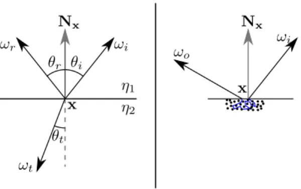
1.2.3 Relation between incident and outgoing quantities
Some relations exist to link incident and outgoing quantities.
Radiance: In free space, a beam’s spectral radiance is conserved at every point:
Lλ,o(x, ω, t) = Lλ,i(x, −ω, t). (1.18)
This equality is valid for any point x which is not on a surface, and every direction ω. On surfaces and in mediums where interactions occur (being gazes or mediums with non-constant refraction indices), the relation is more complex and depends on the local interactions. As the equality is valid for any wavelength, the radiance is also conserved at any point in free space:
Lo(x, ω, t) = Li(x, −ω, t). (1.19)
Irradiance: Rendering models consider that for any time t, thermodynamical equilibrium is reached. This means that each surface point’s temperature is constant during an infinitely small interval dt cen-tered around t. A practical impact of this is that the energy leaving the surface at t only depends on the energy that arrives during an infinitely small amount of time. When a surface point absorbs electro-magnetic energy (or more precisely, the infinitesimal surface around this point absorbs electroelectro-magnetic energy), the temperature at this point increases. When it emits the same amount of energy (possibly in different wavelengths), its temperature decreases by the same amount. Therefore, at thermodynamical equilibrium, a point must emit as much energy as it receives in order to maintain a constant temperature.
1.3. Colorimetry This means that, for any point, the sum of the received energy for all wavelengths must equal the sum of the emitted energy for all wavelengths. This is the same for densities, so we have the following identity:
Eo(x, S2, t) = Ei(x, S2, t), (1.20)
where S2is the unit sphere.
Note that this equality is valid only when considering all the wavelengths when computing irradiance from its spectral counterpart, and does not hold for spectral irradiance. In particular, this is not valid when limiting Λ to the set of visible wavelengths (380nm − 780nm). For instance, surfaces often emit energy in infrared wavelengths, which are then considered as radiant heat by neural sensors in human skin, and responsible for the warm feeling near a hot surface even if not touching it.
Power and energy: as power and energy are defined as the integral of irradiance, the two following equalities apply:
Φo(S, S2, t) = Φi(S, S2, t) (1.21)
Qo(S, S2, T ) = Qi(S, S2, T ) (1.22)
These three last equalities motivate the fact that irradiance, power and energy often appear without an indication about their ingoing or outgoing nature.
1.2.4 Spectral distributions
It is often useful to use spectral radiance or irradiance distributions as one single object. From now on, we will denote L or E (without λ or Λ subscripts) such spectral distributions. They are defined as follows:
L(x, ω, t)(λ) = Lλ(x, ω, t)
E(x, Ω, t)(λ) = Eλ(x, Ω, t)
For any operator f handling spectral quantities, a natural extension to handle spectral distributions is
defined by applying f on each wavelength separately. For instance, (L1+ L2)(λ) = L1(λ) + L2(λ).
1.3
Colorimetry
Radiometry is the framework for electromagnetic energy, and deals with wavelengths and energy. Part of the energy received on a sensor is transformed into an image through a process of perception. This process transforms a distribution of energy with respect to wavelengths into abstract entities, the colors [WS00].
For instance, a thermal sensor will convert the distribution of energy in the infrared wavelengths to colors through a specific perception process, ignoring all other wavelengths. In the case of the human vision system, cones and rods on one side, and the brain on the other side, will transform a distribu-tion of energy density with respect to the visible wavelengths (380nm − 780nm) into a ”mental image” (although it is not formed of pixels). Cones and rods are the sensors, and the brain interprets the mea-surements, the whole being the human vision system (HVS). Put together, this leads to an image, the complete process being perception. In the case of a camera sensor, CCD or CMOS sensors will trans-form this distribution into electric voltage for each pixel, which is then interpreted by specific equipments (software or hardware) to obtain the color of each pixel of the image.
Colorimetry deals with representing colors and giving quantitative tools linked to human perception, as well as switching from energy distributions with respect to the visible wavelengths to colors. It has been established that three type of cones are present in the human eye. Therefore, three numbers are enough to describe any color that can be perceived by the HVS. Note that the transformation from a spectral distribution to a color is not a bijection: several spectral distributions can lead to the same perceived color.
These colors are represented through various so-called color spaces. Some of these spaces can rep-resent all the colors, they are called reference spaces. Some others can only reprep-resent a portion of these colors, but manipulation of colors in these spaces might be easier. In general, all these spaces are shown relatively to a reference space called CIE xyY.
1.3.1 Chromaticity, luminance, gamut
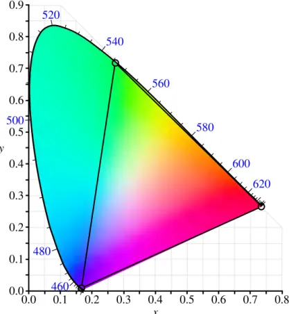
The CIE xyY color space is obtained by splitting a color in two distinct and independent characteris-tics: the luminance Y (which is the perceived brightness of a color), and two chromaticity values, x and y. It is often the case to represent this space using a constant brightness value, which leads to the color schema in Figure 1.3.
Manipulations in the xyY color space are not easy: addition of two colors is not done just by adding each components in a component-wise way, as chromaticity components could be outside of the graph. This is why reference spaces are not used as working color spaces.
Working color spaces can not represent all the colors. For such a color space, the extent of the colors it can represent is called gamut, or color profile. Imaging devices such as printers or screens use specific color spaces, with associated color profiles. When printing an image which is displayed on a screen, the colors must first be converted into the color space of the printer, using a reference space such as xyY as an intermediate to minimize distortion if the color profiles do not match (i.e. , there are colors that can be represented by a screen, but which can not be reproduced by the printer).
1.3.2 RGB, gamma correction, white point, sRGB
RGB color spaces are defined as triangle-shaped spaces inside the chromaticity schema, and are based upon the fact that human eyes have sensors sensitive to red, green and blue colors. To define a RGB color space, it is enough to associate a (x, y) coordinate to each of the RGB coordinates (1, 0, 0), (0, 1, 0) and
1.3. Colorimetry 460 480 500 520 540 560 580 600 620 x 0.0 0.1 0.2 0.3 0.4 0.5 0.6 0.7 0.8 y 0.0 0.1 0.2 0.3 0.4 0.5 0.6 0.7 0.8 0.9
Figure 1.3: CIE xy schema, for a constant luminance Y . This color schema is displayed using a device which does not use a reference space. Therefore, it can not recreate all the colors, which makes the displayed or printed version inexact. Note that the boundary of the graph is made of the colors that are obtained from spectra where a single wavelength is present. Source : Wikipedia.
(0, 0, 1), all the other colors being obtained by interpolating between these colors. As long as all the interpolation weights are positive (the weights being in fact the RGB coordinates), the obtained color chromaticity belongs to the triangle. When the weights sum is 1, the color belongs to the triangle. Otherwise, the luminance is different.
Display devices use RGB color spaces, but at the time of the confection, cathode-ray-tube (CRT) displays were used. In these systems, the process of displaying an image is non-linear in term of bright-ness: an input value twice as large leads to a perceived brightness which is much more than the double. A good approximation of the alteration is that the perceived brightness follows a power law of the form
B = Vγ. To achieve a correct perception, it is therefore necessary to gamma-correct the RGB values,
by applying a transformation of the form Vout = Vin1/γ. In image formats such as JPEG, the
gamma-corrected values are directly stored, as well as the γ value used. Therefore, when using an image as a texture for rendering, where no gamma-correction is needed, the original values must be retrieved first, by applying the inverse transform. A γ value is therefore necessary to further specify a RGB color space. Moreover, a display produces perceived white (equal energy for all wavelengths) for a given maticity value, and a camera associate a given chromaticity for a given spectral distribution. The chro-maticity value for which white should be displayed is called white point. If an image captured with a camera is displayed on a screen with different white point, colors will not appear as expected. A white point is therefore necessary to fully describe a RGB color space.
To summarize, a RGB color space is defined by the (x, y) chromaticity values associated to each of the (1, 0, 0), (0, 1, 0) and (0, 0, 1) RGB coordinates, the gamma correction to apply, and the white point. When two devices do not use the same RGB color spaces, it is necessary to switch from one to another, which can lead to artifacts if one of the characteristic differs largely.
To avoid this and the existence of a lot of different RGB color spaces for printing or screening (one per imaging device), a specific standard RGB color space has been designed: sRGB. This color space is used by most displays and cameras, and is shown in Figure 1.4. Note that the gamut is quite reduced. The D65 point is the white point of sRGB. The particularity of sRGB comes from the fact that the gamma-correction used is not characterized by a single γ value, but is a more intricate function which matches more closely the actual CRT behavior.
1.4
From radiometry to colorimetry
As the simulation phase gives spectral quantities, it is necessary to switch from these spectral data to colors. We focus on two color spaces for which this conversion is possible. The human eye uses cones to translate spectral energy into electric impulses, rods being used for night vision as they are much sen-sitive, at the price of not allowing the brain to perceive colors. It has been established through perceptual studies that three type of cones are used [WS00], each having different sensitivity with respect to wave-lengths. The first type is sensitive to wavelengths around 700nm (which corresponds to reddish colors), the second type is more sensitive to wavelengths around 546nm (green) and the last one is sensitive to wavelengths around 435nm, leading to blue.
1.4. From radiometry to colorimetry 460 480 500 520 540 560 580 600 620 x 0.0 0.1 0.2 0.3 0.4 0.5 0.6 0.7 0.8 y 0.0 0.1 0.2 0.3 0.4 0.5 0.6 0.7 0.8 0.9
Figure 1.4: The interior of the black triangle is the sRGB gamut, i.e. the set of colors that can be repre-sented in the sRGB color space. Source : Wikipedia.
λ 0.40 0.30 0.20 0.10 0.00 -0.10 400 500 600 700 800
Figure 1.5: CIE RGB color matching functions. Note that the red matching function takes negative values, which shows that these functions are not sensitivity models. Source : Wikipedia.
1.4.1 Spectrum → RGB conversion
These observations, together with the will to define a RGB color space, has lead to the definition of specific color-matching functions, which make it possible to compute RGB coefficients for the CIE RGB color space from spectral data. These functions, shown in Figure 1.5, give the contribution of each wavelength to the three main colors (called primary colors), namely red, green and blue.
The associated color space is the CIE RGB color space. The gamut of this space is shown in Fig-ure 1.6. The three main points correspond to spectra with a single wavelength present, the one of the corresponding cone sensitivity peak.
These response functions ¯r(λ), ¯g(λ) and ¯b(λ), are defined over the interval [380nm, 780nm], and
make it possible to obtain the R, G, and B components from a spectral density S(λ) with unit [W.m−2.sr−1.m−1],
which is spectral radiance integrated over time. The three components are obtained as:
R = Z 780nm 380nm S(λ)¯r(λ)dλ (1.23) G = Z 780nm 380nm S(λ)¯g(λ)dλ (1.24) B = Z 780nm 380nm S(λ)¯b(λ)dλ. (1.25)
1.4.2 Spectrum → CIE XYZ → RGB
The conversion method above has problems, as CIE-RGB can not represent all colors. Moreover, display devices do not necessarily use CIE-RGB as color space. Therefore, if the gamut of the device’s color space is not included in the one of CIE-RGB, the conversion will lead to a degradation. It is therefore preferable to represent images with a complete color-space, such as CIE-XYZ, and then convert from this space to the final color space (such as sRGB or any other color space, even subtractive ones based on CMYK, for printers) only when required.
1.4. From radiometry to colorimetry 460 480 500 520 540 560 580 600 620 x 0.0 0.1 0.2 0.3 0.4 0.5 0.6 0.7 0.8 y 0.0 0.1 0.2 0.3 0.4 0.5 0.6 0.7 0.8 0.9
Figure 1.6: CIE RGB color space gamut. This color space includes the sRGB color space.
Sensor plane Image
convolution
Sensor plane Computed image
Figure 1.7: Image and sensor relationship. Left: we associate to each pixel p a point P on the image plane (the spatial extent of the sensor). Right: The value of pixel p in the image is equal to the convolution of a filter centered at P with the signal on the sensor.
This is why the usual conversion pipeline is a bit more complicated than the one presented above. The conversion from a spectrum to CIE-XYZ is done similarly to the conversion from spectra to CIE
RGB, through the use of color-matching functions ¯x, ¯y, ¯z. Note that these matching functions do not
exhibit negative values, as every spectra can be encoded to a valid XYZ triplet.
Then, conversion from CIE-XYZ to the final color space is done through methods which are specific to the final color space. For RGB color spaces, this is usually done through matrices and clamping of negative values.
1.5
Content of a HDR image, sensor
In rendering, the high dynamic range image represents what is measured by a sensor (such as CCD sensors or the retina) [RWPD05]. This sensor is often assumed to be planar, and its spatial extent is called image plane. The high dynamic range image can be seen as a punctual approximation of a 2D continuous signal S representing what is measured on the sensor. S has values in a specific color space, such as CIE-XYZ or sRGB. In rendering, S is the signal obtained by simulating the response of the sensor to the incident radiance, taking into account its sensitivity and other characteristics (directional sensitivity, etc.). The pixel values are then computed such that a continuous signal rebuilt from them is as close as possible from the original signal.
A way to do it is to associate a point P of coordinates (xP, yP) on the sensor to each pixel p, so that
the set of points on the sensor form a regular grid and cover the active zone of the sensor. The value Ip
of the pixel p is then computed as the convolution of the signal with a reconstruction filter hP centered
at point P on the image plane:
Ip =
Z
s(hP)
hP(∆x, ∆y)S(xP + ∆x, yP + ∆y)dA(∆x, ∆y) (1.26)
where s(hP) is the support of the filter hP. Coordinates (∆x = 0, ∆y = 0) correspond to the center of
the filter. The complete process is illustrated in Figure 1.7. Note that the image plane needs to be at least as large as the union of all the filter supports for a correct computation of border pixels.
1.5. Content of a HDR image, sensor -0.4 -0.2 0 0.2 0.4 0.6 0.8 1 -1 -0.5 0 0.5 1
Figure 1.8: 1D Lanczos-sinc filter function on [−1, 1], for increasing values of the τ parameter.
1.5.1 Reconstruction filter
The filter should be normalized (i.e. its integral over s(hP) is equal to 1) to avoid that the range of values
of an HDR image depends on the size of the filter support. It is often the case that the filter’s support of neighboring pixels overlap. Note that the larger the filter support, the more blurry the computed image is. Some known filters in the reconstruction literature are the box filter (the simplest, it is uniform over its support), the triangle filter, or the Gaussian filter. A good approximation of an optimal reconstruction
filter is the Lanczos-sinc filter. Its support has a rectangular shape. Letting u0 and v0 be the (u, v)
coordinates scaled between −1 and 1 in the support, h(u, v) is given by:
h(u, v) = sin(u 0× τ ) u0× τ × sin(u0) u0 × sin(v0× τ ) v0× τ × sin(v0) v0 . (1.27)
τ is a user parameter which controls the global shape of the filter: lower values will make it similar to a Gaussian filter, while larger values will make it oscillate, as illustrated in the 1D-case by Figure 1.8.
1.5.2 Signal value, sensor response
The value S(x, y) of the signal at any point of the image plane (x, y) is obtained by summing the contribution of each light ray hitting the image plane, taking into account the sensor response. On chemical films, photons create splotches, therefore a beam of energy can contribute to a region of the film instead of only contributing to a single point. However, in rendering, it is common to consider that a beam contributes only to the point where it hits the sensor, and we will assume it is the case in the
rest of this document. Depending on the sensor, a directional sensitivity and a wavelength dependency can also be present. However, we assume that the sensor response does not exhibit non-linear effects: its response does not depend on the rays that have been taken into account before. The effect of this behavior would not be negligible if the sensor to simulate was easily saturated, its response decreasing with the amount of energy already absorbed, but we assume that our sensor does not have such properties. As we additionally consider that no cross-wavelength interactions occur and that the response is the same for each point of the sensor, the response function can be modeled as a simple direction-dependent spectral distribution weighting function R(ω).
A sensor produces measures in a given color space. We take CIE-XYZ as it is a complete space, which avoids color-loss (Section 1.4.2). Therefore, S(x, y) is a XYZ triplet. Each component of this color space value is obtained by summing the spectral contributions for each incident direction and each time value. For instance for the X component:
SX(x, y) = Z T Z S2 Z Λ ¯ x((R(ω)dEi(x, y, ω, t))(λ)dλdt (1.28)
where the fact that the measure is done after the photons have hit the sensor’s surface is taken into account
by considering dEi(x0, y0, ω, t) instead of Li(x0, y0, ω, t). Y and Z are computed using similar equations.
If the direction has no effect (i.e. , R(ω) = 1 ∀ω), the expression can be further simplified:
SX(x, y) = Z T Z S2 Z Λ ¯ x((R(ω)dEi(x, y, ω, t))(λ)dλdt = Z T Z Λ ¯ x(λ)Eλ,i(x, y, S2, t)dλdt
and similarly for the Y and Z components. If the response function is independent from the direction, spectral irradiance can be used directly instead of dealing with spectral radiance when computing the final signal value.
1.6
Light interactions
Now that measurement of energy and conversion to colors by a sensor is described, we have to know how it reached the sensor in the first place. Light reaching the sensor has been emitted by light sources, and gone through interactions with the elements of the scene: objects, gazes, etc.. Light can interact in three ways with matter: it can be self-emitted, absorbed or scattered. Each of these interactions are best described intuitively at the photon level, but are handled in a statistic fashion in radiometry.
1.6.1 Self-emission
In real world, photons can be created through several atomic processes. We present incandescence to illustrate a way of creating photons, as it is one of the most common type of emission used. As a matter of fact, incandescence is responsible for the emission of light by light bulbs and hot gazes.
![Figure 1.8: 1D Lanczos-sinc filter function on [−1, 1], for increasing values of the τ parameter.](https://thumb-eu.123doks.com/thumbv2/123doknet/2096100.7552/39.892.207.715.135.546/figure-lanczos-sinc-filter-function-increasing-values-parameter.webp)