Conjoint measurement tools for MCDM, A brief introduction

Laboratoire d'Analyse et Modélisation de Systèmes pour l'Aide à la Décision CNRS UMR 7024

CAHIER DU LAMSADE

210

Conjoint measurement tools for MCDM. A brief introduction D. Bouyssou, M. Pirlot

Conjoint measurement tools for MCDM

A brief introduction

1

Denis Bouyssou

CNRS – LAMSADE

Marc Pirlot

Facult´e Polytechnique de Mons

Revised 21 May 2003

1_{Part of this work was accomplished while Denis Bouyssou was visiting the}

Ser-vice de Math´ematique de la Gestion at the Universit´e Libre de Bruxelles (Brussels,

Belgium). The warm hospitality of the Service de Math´ematique de la Gestion, the support of the Belgian Fonds National de la Recherche Scientistic and the Brussels-Capital Region through a “Research in Brussels” action grant are grate-fully acknowledged. Many Figures in this text were inspired by [77].

2_{LAMSADE, Universit´e Paris Dauphine, Place du Mar´echal de Lattre de}

Tas-signy, F-75775 Paris Cedex 16, France, tel: +33 1 44 05 48 98, fax: +33 1 44 05 40 91, e-mail: bouyssou@lamsade.dauphine.fr, Corresponding author.

3_{Facult´e Polytechnique de Mons, 9, rue de Houdain, B-7000 Mons, Belgium,}

Abstract

This paper offers a brief and nontechnical introduction to the use of con-joint measurement in multiple criteria decision making. The emphasis is on the, central, additive value function model. We outline its axiomatic foun-dations and present various possible assessment techniques to implement it. Some extensions of this model, e.g. nonadditive models or models tolerating intransitive preferences are then briefly reviewed.

Keywords: Conjoint Measurement, Additive Value Function, Preference Modelling.

1

Introduction and motivation

Conjoint measurement is a set of tools and results first developed in Eco-nomics [41] and Psychology [127] in the beginning of the ‘60s. Its, ambitious, aim is to provide measurement techniques that would be adapted to the needs of the Social Sciences in which, most often, multiple dimensions have to be taken into account.

Soon after its development, people working in decision analysis realized that the techniques of conjoint measurement could also be used as tools to structure preferences [46, 148]. This is the subject of this paper which offers a brief and nontechnical introduction to conjoint measurement models and their use in multiple criteria decision making. More detailed treatments may be found in [57, 72, 108, 121, 191]. Advanced references include [52, 115, 193].

1.1

Conjoint measurement models in Decision Theory

The starting point of most works in Decision Theory is a binary relation % on a set A of objects. This binary relation is usually interpreted as an “at least as good as” relation between alternative courses of action gathered in A.

Manipulating a binary relation can be quite cumbersome as soon as the set of objects is large. Therefore, it is not surprising that many works have looked for a numerical representation of the binary relation %. The most obvious numerical representation amounts to associate a real number V (a) to each object a ∈ A in such a way that the comparison between these numbers faithfully reflects the original relation %. This leads to defining a real-valued function V on A, such that:

a % b ⇔ V (a) ≥ V (b), (1)

for all a, b ∈ A. When such a numerical representation is possible, one can use V in lieu of % and, e.g. apply classical optimization techniques to find the most preferred elements in A given %. We shall call such a function V a value function.

It should be clear that not all binary relations % may be represented by a value function. Condition (1) imposes that % is complete (i.e. a % b or b % a, for all a, b ∈ A) and transitive (i.e. a % b and b % c imply a % c, for all a, b, c ∈ A). When A is finite or countably infinite, it is well-known [52, 115] that these two conditions are, in fact, not only necessary but also sufficient to build a value function satisfying (1).

Remark 1

The general case is more complex since (1) implies, for instance, that there must be “enough” real numbers to distinguish objects that have to be dis-tinguished. The necessary and sufficient conditions for (1) can be found in [52, 115]. An advanced treatment is [13]. Sufficient conditions that are well-adapted to cases frequently encountered in Economics can be found in

[39]. •

It is vital to note that, when a value function satisfying (1) exists, it is by no means unique. Taking any increasing function φ on R, it is clear that φ ◦ V gives another acceptable value function. A moment of reflection will convince the reader that only such transformations are acceptable and that if V and U are two real-valued function on A satisfying (1), they must be related by an increasing transformation. In other words, a value function in the sense of (1) defines an ordinal scale.

Ordinal scales, although useful, do not allow the use of sophisticated assessment procedures, i.e. of procedures that allow an analyst to assess the relation % through a structured dialogue with the decision-maker. This is because the knowledge that V (a) ≥ V (b) is strictly equivalent to the knowledge of a % b and no inference can be drawn from this assertion besides the use of transitivity.

It is therefore not surprising that much attention has been devoted to numerical representations leading to more constrained scales. Many possible avenues have been explored to do so. Among the most well-know, let us mention:

• the possibility to compare probability distributions on the set A [52, 189]. If it is required that, not only (1) holds but that the numbers attached to the objects should be such that their expected values re-flects the comparison of probability distributions on the set of objects, a much more constrained numerical representation clearly obtains, • the introduction of “preference difference” comparisons of the type: the

difference between a and b is larger than the difference between c and d, see [41, 115, 163, 181]. If it is required that, not only (1) holds, but that the differences between numbers also reflect the comparisons of preference differences, a more constrained numerical representation obtains.

When objects are evaluated according to several dimensions, i.e. when % is defined on a product set, new possibilities emerge to obtain numerical repre-sentations that would specialize (1). The purpose of conjoint measurement is to study such kinds of models.

There are many situations in decision theory which call for the study of binary relations defined on product sets. Among them let us mention:

• Multiple criteria decision making using a preference relation comparing alternatives evaluated on several attributes [15, 108, 145, 156, 191], • Decision under uncertainty using a preference relation comparing

alter-natives evaluated on several states of nature [62, 95, 160, 167, 192, 193], • Micro Economics manipulating preference relations for bundles of

sev-eral goods [40],

• Dynamic decision making using a preference relation between alterna-tives evaluated at several moments in time [108, 111, 112],

• Social choice comparing distribution of wealth across several individu-als [5, 16, 17, 198].

The purpose of this paper is to give an introduction to the main models of conjoint measurement useful in multiple criteria decision making. The results and concepts that are presented may however be of interest in all of the afore-mentioned areas of research.

Remark 2

Restricting ourselves to applications in multiple criteria decision making will not allow us to cover every aspects of conjoint measurement. Among the most important topics left aside, let us mention: the introduction of statistical elements in conjoint measurement models [49, 96] and the test of conjoint

measurement models in experiments [121]. •

Given a binary relation % on a product set X = X1× X2× · · · × Xn, the theory of conjoint measurement consists in finding conditions under which it is possible to build a convenient numerical representation of % and to study the uniqueness of this representation. The central model is the additive value function model in which:

x % y ⇔ n X i=1 vi(xi) ≥ n X i=1 vi(yi) (2)

where vi are real-valued functions, called partial value functions, on the sets Xi and it is understood that x = (x1, x2, . . . , xn) and y = (y1, y2, . . . , yn). Clearly if % has a representation in model (2), taking any common increasing transformation of the vi will not lead to another representation in model (2). Specializations of this model in the above-mentioned areas give several central models in decision theory:

• The Subjective Expected Utility model, in the case of decision-making under uncertainty,

• The discounted utility model for dynamic decision making,

• Inequality measures `a la Atkinson/Sen in the area of social welfare. The axiomatic analysis of this model is now quite firmly established [41, 115, 193]; this model forms the basis of many decision analysis techniques [72, 108, 191, 193]. This is studied in sections 3 and 4 after we introduce our main notation and definitions in section 2.

Remark 3

One possible objection to the study of model (2) is that the choice of an additive model seems arbitrary and restrictive. It should be observed here that the functions vi will precisely be assessed so that additivity holds.

It is also useful to notice that this model can be reformulated so as to make addition disappear. Indeed if there are partial value functions vi such that (2) holds, it is clear that V =Pn

i=1vi is a value function satisfying (1). Now, since V defines an ordinal scale, taking the exponential of V leads to another valid value function W . Clearly W has now a multiplicative form:

x % y ⇔ W (x) = n Y i=1 wi(xi) ≥ W (y) = n Y i=1 wi(yi). where wi(xi) = evi(xi).

The reader is referred to chapter XXX (Chapter 6, Dyer) for the study of situations in which V defines a scale that is more constrained than an ordinal scale, e.g. because it is supposed to reflect preference differences or because it allows to compute expected utilities. In such cases, the additive form (2) is no more equivalent to the multiplicative form envisaged above. • In section 5 we envisage a number of extensions of this model going from nonadditive representations of transitive relations to model tolerating intran-sitive indifference and, finally, nonadditive representations of nontranintran-sitive relations.

Remark 4

We shall limit our attention in this paper to the case in which alternatives may be evaluated on the various attributes without risk or uncertainty. Ex-cellent overviews of these cases may be found in [108, 191]. •

Before starting our study of conjoint measurement oriented towards MCDM, it is worth recalling that conjoint measurement aims at establishing measure-ment models in the Social Sciences. To many, the very notion of “measure-ment in the Social Sciences” may appear contradictory. It may therefore be

useful to briefly envisage how the notion of measurement can be modelled in the realm of Physics and to explain how a “measurement model” may indeed be useful in order to structure preferences.

1.2

An aside: measuring length

Physicists usually take measurement for granted and are not particularly concerned with the technical and philosophical issues it raises (at least when they work within the realm of Newtonian Physics). However, for a Social Scientist, these question are of utmost importance. It may thus help to have an idea of how things appear to work in Physics before tackling more delicate cases.

Suppose that you are on a desert island and that you want to “measure” the length of a collection of rigid straight rods. Note that we do not discuss here the “pre-theoretical” intuition that “length” is a property of these rods that can be measured, as opposed, say, to their rigidity, their softness or their beauty.

r r0

r  r0 s s

0 s ∼ s0

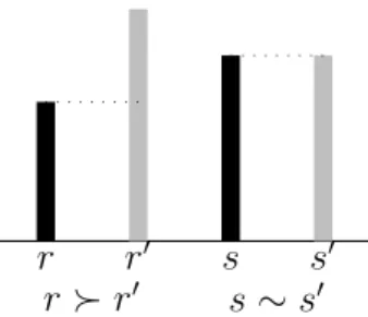
Figure 1: Comparing the length of two rods.

A first simple step in the construction of a measure of length is to place the two rods side by side in such a way that one of their extremities is at the same level (see Figure 1). Two things may happen: either the upper extremities of the two rods coincide or not. This seems to be the simplest way to devise an experimental procedure leading to the discovery of which rod “has more length” than the other. Technically, this leads to defining two binary relations  and ∼ on the set of rods in the following way:

r  r0 when the extremity of r is higher than the extremity of r0, r ∼ r0 when the extremities of r and r0 are at the same level,

Clearly, if length is a quality of the rods that can be measured, it is expected that these pairwise comparisons are somehow consistent, e.g.,

• if r  r0 _{and r}0 _{ r}00_{, it should follow that r  r}00_, • if r ∼ r0 _{and r}0 _{∼ r}00_{, it should follow that r ∼ r}00_, • if r ∼ r0 _{and r}0 _{ r}00_{, it should follow that r  r}00_.

Although quite obvious, these consistency requirements are stringent. For instance, the second and the third conditions are likely to be violated if the experimental procedure involves some imprecision, e.g if two rods that slightly differ in length are nevertheless judged “equally long”. They repre-sent a form of idealization of what could be a perfect experimental procedure. With the binary relations  and ∼ at hand, we are still rather far from a full-blown measure of length. It is nevertheless possible to assign numbers to each of the rods in such a way that the comparison of these numbers reflects what has been obtained experimentally. When the consistency requirements mentioned above are satisfied, it is indeed generally possible to build a real-valued function Φ on the set of rods that would satisfy:

r  r0 ⇔ Φ(r) > Φ(r0) and r ∼ r0 ⇔ Φ(r) = Φ(r0).

If the experiment is costly or difficult to perform, such a numerical assignment may indeed be useful because it summarizes, once for all, what has been obtained in experiments. Clearly there are many possible ways to assign numbers to rods in this way. Up to this point, they are equally good for our purposes. The reader will easily check that defining % as  or ∼, the function Φ is noting else than a “value function” for length: any increasing transformation may therefore be applied to Φ.

r and s r0 _{and s}0

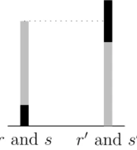
Figure 2: Comparing the length of composite rods.

The next major step towards the construction of a measure of length is the realization that it is possible to form new rods by simply placing two or more rods “in a row”, i.e. you may concatenate rods. From the point of view

of length, it seems obvious to expect this concatenation operation ◦ to be “commutative” (r ◦ s has the same length as s ◦ r) and associative ((r ◦ s) ◦ t has the same length as r ◦ (s ◦ t)).

You clearly want to be able to measure the length of these composite ob-jects and you can always include them in in our experimental procedure out-lined above (see Figure 2). Ideally, you would like your numerical assignment Φ to be somehow compatible with the concatenation operation: knowing the numbers assigned to two rods, you want to be able to deduce the number assigned to their concatenation. The most obvious way to achieve that is to require that the numerical assignment of a composite object can be deduced by addition from the numerical assignments of the objects composing it, i.e. that

Φ(r ◦ r0) = Φ(r) + Φ(r0).

This clearly places many additional constraints on the results of your experi-ment. One obvious one is that  and ∼ should somehow be compatible with the concatenation operation ◦, e.g.

r  r0 and t ∼ t0 should lead to r ◦ t  r0 ◦ t0.

These new constraints may or not be satisfied. When they are, the usefulness of the numerical assignment Φ is even more apparent: a simple arithmetic operation will allow to infer the result of an experiment involving composite objects.

Let us take a simple example. Suppose that you have 5 rods r1, r2, . . . , r5 and that, because space is limited, you can only concatenate at most two rods and that not all concatenations are possible. Let us suppose, for the moment, that you do not have much technology available so that you may only experiment using different rods. You may well collect the following information, using obvious notation exploiting the transitivity of  which holds in this experiment,

r1◦ r5 Â r3 ◦ r4 Â r1◦ r2 Â r5 Â r4 Â r3 Â r2 Â r1.

Your problem is then to find a numerical assignment Φ to rods such that using an addition operation, you can infer the numerical assignment of composite objects consistently with your observations. Let us envisage the following three assignments:

Φ Φ0 _Φ00 r1 14 10 14 r2 15 91 16 r3 20 92 17 r4 21 93 18 r5 28 100 29

These three assignments are equally valid to reflect the comparison of single rods. Only the first and the third allow to capture the comparison of compos-ite objects. Note that, going from Φ to Φ00 _{does not involve just changing the} “unit of measurement”: since Φ(r1) = Φ00(r1) this would imply that Φ = Φ00, which is clearly false. This implies that such numerical assignments have limited usefulness. Indeed, it is tempting to use them to predict the result of comparisons that we have not been able to perform. But this turns out to be quite disappointing: using Φ you would conclude that r2◦ r3 ∼ r1◦ r4 since Φ(r2) + Φ(r3) = 15 + 20 = 35 = Φ(r1) + Φ(r4), but, using Φ00, you would conclude that r2 ◦ r3 Â r1◦ r4 since Φ00(r2) + Φ00(r3) = 16 + 17 = 33 while Φ00_(r

1) + Φ00(r4) = 14 + 18 = 32.

Intuitively, “measuring” calls for some kind of a standard (e.g. the “M`etre-´etalon” that can be found in the Bureau International des Poids et Mesures in S`evres, near Paris). This implies choosing an appropriate “standard” rod and being able to prepare perfect copies of this standard rod (we say here “appropriate” because the choice of a standard should be made in accordance with the lengths of the objects to be measured: a tiny or a huge standard will not facilitate experiments). Let us call s0 the standard rod. Let us suppose that you have been able to prepare a large number of perfect copies s1, s2, . . . of s0. We therefore have:

s0 ∼ s1, s0 ∼ s2, s0 ∼ s3, . . .

Let us also agree that the length of s0 is 1. This is your, arbitrary, unit of length. How can you use s0 and its perfect copies so as to determine unambiguously the length of any other (simple or composite) object? Quite simply, you may prepare a “standard sequence of length n”, S(n) = s1◦ s2◦ . . . ◦ sn−1◦ sn, i.e. a composite object that is made by concatenating n perfect copies of our standard rod s0. The length of a standard sequence of length n is exactly n since we have concatenated n objects that are perfect copies of the standard rod of length 1. Take any rod r and let us now compare r with several standard sequences of increasing length: S(1), S(2), . . .

Two cases may arise. There may be a standard sequence S(k) such that r ∼ S(k). In that case, we know that the number Φ(r) assigned to r must be exactly k. This is unlikely however. The most common situation is that

we will find two consecutive standard sequences S(k − 1) and S(k) such that r  S(k − 1) and S(k)  r (see Figure 3). This means that Φ(r) must be such that k − 1 < Φ(r) < k. We seem to be in trouble here since, as before, Φ(r) is not exactly determined. How can you proceed? This depends on your technology for preparing perfect copies.

r S(k) s1 s2 s3 s4 s5 s6 s7 s8 r  S(7), S(8)  r 7 < Φ(r) < 8

Figure 3: Using standard sequences.

Imagine that you are able to prepare perfect copies not only of the stan-dard rod but also of any object. You may then prepare several copies (r1, r2, . . .) of the rod r. You can now compare a composite object made out of two perfect copies of r with your standard sequences S(1), S(2), . . . As before, you shall eventually arrive at locating Φ(r1◦ r2) = 2Φ(r) within an interval of width 1. This means that the interval of imprecision surrounding Φ(r) has been divided by two. Continuing this process, considering longer and longer sequences of perfect copies of r, you will keep on reducing the width of the interval containing Φ(r). This means that you can approximate Φ(r) with any given level of precision. Mathematically a unique value for Φ(r) will be obtained using a simple limiting argument.

Supposing that you are in position to prepare perfect copies of any object is a strong technological requirement. When this is not possible, there still exists a way out. Instead of preparing a perfect copy of r you may also try to increase the granularity of your standard sequence. This means building an object t that you would be able to replicate perfectly and such that con-catenating t with one of its perfect replicas gives an object that has exactly the length of the standard object s0, i.e. Φ(t) = 1/2. Now considering stan-dard sequences based on t, you will be able to increase by a factor 2 the precision with which we measure the length of r. Repeating the process, i.e. subdividing t, will lead, as before, to a unique limiting value for Φ(r).

The mathematical machinery underlying the measurement process infor-mally described above (called “extensive measurement”) rests on the theory

of ordered groups. It is beautifully described and illustrated in [115]. Al-though the underlying principles are simple, we may expect complications to occur e.g. when not all concatenations are feasible, when there is some level (say the velocity of light if we were to measure speed) that cannot be exceeded or when it comes to relate different measures. See [115, 126, 151] for a detailed treatment.

Clearly, this was an overly detailed and unnecessary complicated descrip-tion of how length could be measured. Since our aim is to eventually deal with “measurement” in the Social Sciences, it may however be useful to keep the above process in mind. Its basic ingredients are the following:

• well-behaved relations  and ∼ allowing to compare objects,

• a concatenation operation ◦ allowing to consider composite objects, • consistency requirements linking Â, ∼ and ◦,

• the ability to prepare perfect copies of some objects in order to build standard sequences.

Basically, conjoint measurement is a quite ingenious way to perform re-lated measurement operations when no concatenation operation is available. This will however require that objects can be evaluated along several dimen-sions. Before explaining how this might work, it is worth explaining the context in which such measurement might prove useful.

Remark 5

It is often asserted that “measurement is impossible in the Social Sciences” precisely because the Social Scientist has no way to define a concatenation operation. Indeed, it would seem hazardous to try to concatenate the in-telligence of two subjects or the pain of two patients. Even, when there seems to be a concatenation operation readily available, it does not always fit the purposes of extensive measurement. Consider for instance an indi-vidual expressing preferences for the quantity of the 2 goods he consumes. The objects therefore take the well structured form of points in the posi-tive orthant of R2_{. There seems to be an obvious concatenation operation} here: (x, y) ◦ (z, w) might simply be taken to be (x + y, z + w). However a fairly rational person, consuming pants and jackets, may indeed prefer (3, 0) (3 pants and no jacket) to (0, 3) (no pants and 3 jackets) but at the same time prefer (3, 3) to (6, 0). This implies that these preferences can-not be explained by a measure that would be additive with respect to the concatenation operation consisting in adding the quantities of the two goods consumed. Indeed (3, 0) Â (0, 3) implies Φ(3, 0) > Φ(0, 3), which implies

Φ(3, 0) + Φ(3, 0) > Φ(0, 3) + Φ(3, 0). Additivity with respect to concatena-tion should then imply that (3, 0)◦(3, 0) Â (0, 3)◦(3, 0) that is (6, 0) Â (3, 3). The power of conjoint measurement will precisely be to provide a means to bypass this absence of readily available concatenation operation as soon

as the objects are evaluated on several dimensions. •

1.3

An example: Even swaps

The even swaps technique described and advocated in [107, 108, 148] is a simple way to deal with decision problems involving several attributes that do not have recourse to a formal representation of preferences, which will be the subject of conjoint measurement. Because this technique is simple and may be quite useful, we describe it below using the same example as in [107]. This will also allow to exemplify the type of problems that are dealt with in decision analysis applications of conjoint measurement.

Example 6 (Even swaps technique)

A consultant considers renting a new office. Five different locations have been identified after a careful consideration of many possibilities, rejecting all those that do not meet a number of requirements.

His feeling is that five distinct characteristics, we shall say five attributes, of the possible locations should enter into his decision: his daily commute time (expressed in minutes), the ease of access for his clients (expressed as the percentage of his present clients living close to the office), the level of services offered by the new office (expressed on an ad hoc scale with three levels: A (all facilities available), B (telephone and fax), C (no facilities)), the size of the office expressed in square feet, and the monthly cost expressed in dollars.

The evaluation of the five offices is given in Table 1 The consultant has

a b c d e Commute 45 25 20 25 30 Clients 50 80 70 85 75 Services A B C A C Size 800 700 500 950 700 Cost 1850 1700 1500 1900 1750

Table 1: Evaluation of the 5 offices on the 5 attributes.

well-defined preferences on each of these attributes. His preference increases with the level of access for his clients, the level of services of the office and

its size. It decreases with commute time and cost. This gives a first easy way to compare alternatives through the use of dominance.

An alternative y is dominated by an alternative x if x is at least as good as y on all attributes while being strictly better for at least one attribute. Clearly dominated alternatives are not candidate for the final choice and may, thus, be dropped from consideration. The reader will easily check that, on this example, alternative b dominates alternative e: e and b have similar size but b is less expensive, involves a shorter commute time, an easier access to clients and a better level of services. We may therefore forget about alternative e. This is the only case of “pure dominance” in our table. It is however easy to see that d is “close” to dominating a, the only difference in favor of a being on the cost attribute (50 $ per month). This is felt more than compensated by the differences in favor of d on all other attributes: commute time (20 minutes), client access (35 %) and size (150 sq. feet).

Dropping now all alternatives that are not candidate for choice, this initial investigation allows to reduce the problem to:

b c d Commute 25 20 25 Clients 80 70 85 Services B C A Size 700 500 950 Cost 1700 1500 1900

A natural way to proceed is then to assess trade-offs. Observe that all alter-natives but b have a common evaluation on commute time. We may therefore ask the consultant, starting with office c, what gain on client access would compensate a loss of 5 minutes on commute time. We are looking for an alternative c0 _{that would be evaluated as follows:}

c c0 Commute 20 25 Clients 70 70 + δ Services C C Size 500 500 Cost 1500 1500

and judged indifferent to c. Although this is not an easy question, it is clearly crucial in order to structure preferences.

Remark 7

We do not envisage in this paper the possibility of lexicographic preferences, in which such tradeoffs do not occur, see [53, 54, 143]. Lexicographic pref-erences may also be combined with the possibility of “local” tradeoffs, see

Suppose that the answer is that for δ = 8, it is reasonable to assume that c and c0 _{would be indifferent. This means that the decision table can now be} reformulated as follows: b c0 _d Commute 25 25 25 Clients 80 78 85 Services B C A Size 700 500 950 Cost 1700 1500 1900

It is then apparent that all alternatives have a similar evaluation on the first attribute which, therefore, is not useful to discriminate between alternatives and may be forgotten. The reduced decision table is now as follows:

b c0 _d

Clients 80 78 85

Services B C A

Size 700 500 950

Cost 1700 1500 1900

There is no case of dominance in this reduced table. Therefore further simpli-fication calls for the assessment of new tradeoffs. Using cost as the reference attribute, we then proceed to “neutralize” the service attribute. Starting with office c0_{, this means asking for the increase in monthly cost that the} consultant would just be prepared to pay to go from level “C” of service to level “B”. Suppose that this increase is roughly 250 $. This defines alterna-tive c00_{. Similarly, starting with office d we ask for the reduction of cost that} would exactly compensate a reduction of services from “A” to “B”. Suppose that the answer is 100 $ a month, which defines alternative d0. The decision table is now reshaped as:

b c00 _d0

Clients 80 78 85

Services B B B

Size 700 500 950

Cost 1700 1750 1800

We may now forget about the second attribute which does not discriminate any more between alternatives. When this is done, it is apparent that c00 _is now dominated by b and can be suppressed. Therefore, the decision table at this stage looks like the following:

b d0

Clients 80 85

Size 700 950

Cost 1700 1800

Unfortunately, this table reveals no case of dominance. New tradeoffs have to be assessed. We may now ask, starting with office b, what additional cost the consultant would be ready to incur to increase its size by 250 square feet. Suppose that the rough answer is 250 $ a month, which defines b0_{. We are} now facing the following table:

b0 _d0

Clients 80 85

Size 950 950

Cost 1950 1800

Attribute size may now be dropped from consideration. But, when this is done, it is clear that d0 _{dominates b}0_{. Hence it seems obvious to recommend}

office d as the final choice. 3

The above process is simple and looks quite obvious. If this works, why be interested at all in “measurement” if the idea is to help someone to come up with a decision?

First observe that in the above example, the set of alternatives was rel-atively small. In many practical situations, the set of objects to compare is much larger than the set of alternatives in our example. Using the even swaps technique could then require a considerable number of difficult tradeoff ques-tions. Furthermore, as the output of the technique is not a preference model but just the recommendation of an alternative in a given set, the appear-ance of new alternatives (e.g. because a new office is for rent) would require starting a new round of questions. This is likely to be highly frustrating. Finally, the informal even swaps technique may not be well adapted to the, many, situations, in which the decision under study takes place in a complex organizational environment. In such situations, having a formal model to be able to communicate and to convince is an invaluable asset. Such a model will furthermore allow to conduct extensive sensitivity analysis and, hence, to deal with imprecision both in the evaluations of the objects to compare and in the answers to difficult questions concerning tradeoffs.

This clearly leaves room for a more formal approach to structure prefer-ences. But where can “measurement” be involved in the process? It should be observed that, beyond surface, there are many analogies between the even swap process and the measurement of length envisaged above.

First, note that, in both cases, objects are compared using binary rela-tions. In the measurement of length, the binary relation  reads “is longer than”. Here it reads “is preferred to”. Similarly, the relation ∼ reading be-fore “has equal length” now reads “is indifferent to”. We supposed in the measurement of length process that  and ∼ would nicely combine in exper-iments: if r  r0 _{and r}0 _{∼ r}00 _{then we should observe that r  r}00_{. Implicitly,} a similar hypothesis was made in the even swaps technique. To realize that this is the case, it is worth summarizing the main steps of the argument.

We started with the following decision table 1. Our overall recommenda-tion was to rent office d. This means that we have reason to believe that d is preferred to all other potential locations, i.e. d  a, d  b, d  c, and d  e. How did we arrive logically at such a conclusion?

Based on the initial table, using dominance and quasi-dominance, we concluded that b was preferable to e and that d was preferable to a. Using symbols, we have b  e and d  a. After assessing some tradeoffs, we concluded, using dominance, that b  c00_{. But remember, c}00 _{was built so as} to be indifferent to c0 _{and, in turn, c}0 _{was built so as to be indifferent to c.} That is, we have c00 _{∼ c}0 _{and c}0 _{∼ c. Later, we built an alternative d}0 _{that is} indifferent to d (d ∼ d0_{) and an alternative b}0 _{that is indifferent to b (b ∼ b}0_). We then concluded, using dominance, that d0 _{was preferable to b}0 _(d0 _{ b}0_). Hence, we know that:

d  a, b  e, c00∼ c0, c0 ∼ c, b  c00, d ∼ d0, b ∼ b0, d0  b0.

Using the consistency rules linking  and ∼ that we envisaged for the mea-surement of length, it is easy to see that the last line implies d  b. Since b  e, this implies d  e. It remains to show that d  c. But the second line leads to, combining  and ∼, b  c. Therefore d  b leads to d  c and we are home. Hence, we have used the same properties for preference and indifference as the properties of “is longer than” and “has equal length” that we hypothesized in the measurement of length.

Second it should be observed that expressing tradeoffs leads, indirectly, to equating the “length” of “preference intervals” on different attributes. Indeed, remember how c0 _{was constructed above: saying that c and c}0 _are indifferent more or less amounts to saying that the interval [25, 20] on com-mute time has exactly the same “length” as the interval [70, 78] on client access. Consider now an alternative f that would be identical to c except that it has a client access at 78%. We may again ask which increase in client access would compensate a loss of 5 minutes on commute time. In a tabular

form we are now comparing the following two alternatives: f f0 Commute 20 25 Clients 78 78 + δ Services C C Size 500 500 Cost 1500 1500

Suppose that the answer is that for δ = 10, f and f0 _{would be indifferent.} This means that the interval [25, 20] on commute time has exactly the same length as the interval [78, 88] on client access. Now, we know that the prefer-ence intervals [70, 78] and [78, 88] have the same “length”. Hprefer-ence, tradeoffs provide a means to equate two preference intervals on the same attribute. This brings us quite close to the construction of standard sequences. This, we shall shortly do.

How does this information about the “length” of preference intervals re-late to judgements of preference or indifference? Exactly as in the even swaps technique. You can use this measure of “length” modifying alternatives in such a way that they only differ on a single attribute and then use a simple dominance argument.

Conjoint measurement techniques may roughly be seen as a formaliza-tion of the even swaps technique that leads to building a numerical model of preferences much in the same way that we built a numerical model for length. This will require assessment procedures that will rest on the same principles as the standard sequence technique used for length. This process of “measuring preferences” is not an easy one. It will however lead to a numerical model of preference that will not only allow us to make a choice within a limited number of alternatives but that can serve as an input of computerized optimization algorithms that will be able to deal with much more complex cases.

2

Definitions and notation

Before entering into the details of how conjoint measurement may work, a few definitions and notation will be needed.

2.1

Binary relations

A binary relation % on a set A is a subset of A × A. We write a % b instead of (a, b) ∈ %. A binary relation % on A is said to be:

• reflexive if [a % a],

• complete if [a % b or b % a], • symmetric if [a % b] ⇒ [b % a], • asymmetric if [a % b] ⇒ [N ot[b % a]], • transitive if [a % b and b % c] ⇒ [a % c],

• negatively transitive if [ N ot[ a % b ] and N ot[ b % c ] ] ⇒ N ot[ a % c ] , for all a, b, c ∈ A.

The asymmetric (resp. symmetric) part of % is the binary relation  (resp. ∼) on A defined letting, for all a, b ∈ A, a  b ⇔ [a % b and N ot(b % a)] (resp. a ∼ b ⇔ [a % b and b % a]). A similar convention will hold when % is subscripted and/or superscripted.

A weak order (resp. an equivalence relation) is a complete and transitive (resp. reflexive, symmetric and transitive) binary relation. For a detailed analysis of the use of binary relation as tools for preference modelling we refer to [4, 52, 60, 144, 150, 152]. The weak order model underlies the examples that were presented in introduction. Indeed, the reader will easily prove the following.

Proposition 8

Let % be a weak order on A. Then: • Â is transitive,

• Â is negatively transitive, • ∼ is transitive,

• [a  b and b ∼ c] ⇒ a  c, • [a ∼ b and b  c] ⇒ a  c.

2.2

Binary relations on product sets

In the sequel, we consider a set X = Qn

i=1Xi with n ≥ 2. Elements x, y, z, . . . of X will be interpreted as alternatives evaluated on a set N = {1, 2, . . . , n} of attributes. A typical binary relation on X is still denoted as %, interpreted as an “at least as good as” preference relation between multi-attributed al-ternatives with ∼ interpreted as indifference and  as strict preference.

For any non empty subset J of the set of attributes N , we denote by XJ (resp. X−J) the set Qi∈JXi (resp. Qi /∈JXi ). With customary abuse of notation, (xJ, y−J) will denote the element w ∈ X such that wi = xi if i ∈ J and wi = yi otherwise. When J = {i} we shall simply write X−i and (xi, y−i).

Remark 9

Throughout this paper, we shall work with a binary relation defined on a product set. This setup conceals the important work that has to be done in practice to make it useful:

• the structuring of objectives [3, 14, 15, 104, 105, 106, 141, 146],

• the definition of adequate attributes to measure the attainment of ob-jectives [73, 85, 103, 109, 156, 190, 197],

• the definition of an adequate family of attributes [22, 108, 156, 157, 191],

• the modelling of uncertainty, imprecision and inaccurate determination [21, 25, 108, 154].

The importance of this “preliminary” work should not be forgotten in what

follows. •

2.3

Independence and marginal preferences

In conjoint measurement, one starts with a preference relation % on X. It is then of vital importance to investigate how this information makes it possible to define preference relations on attributes or subsets of attributes.

Let J ⊆ N be a nonempty set of attributes. We define the marginal relation %J induced on XJ by % letting, for all xJ, yJ ∈ XJ:

xJ %J yJ ⇔ (xJ, z−J) % (yJ, z−J), for all z−J ∈ X−J,

with asymmetric (resp. symmetric) part ÂJ (resp. ∼J). When J = {i}, we often abuse notation and write %i instead of %{i}. Note that if % is reflexive (resp. transitive), the same will be true for %J. This is clearly not true for completeness however.

Definition 10 (Independence)

Consider a binary relation % on a set X = Qn

i=1Xi and let J ⊆ N be a nonempty subset of attributes. We say that % is independent for J if, for all xJ, yJ ∈ XJ,

If % is independent for all non empty subsets of N , we say that % is inde-pendent. If % is independent for all subsets containing a single attribute, we say that % is weakly independent.

In view of (2), it is clear that the additive value model will require that % is independent. This crucial condition says that common evaluations on some attributes do not influence preference. Whereas independence implies weak independence, it is well-know that the converse is not true [193]. Remark 11

Independence, or at least weak independence, is an almost universally ac-cepted hypothesis in multiple criteria decision making. It cannot be overem-phasized that it is easy to find examples in which it is inadequate.

If a meal is described by the two attributes, main course and wine, it is highly likely that most gourmets will violate independence, preferring red wine with beef and white wine with fish. Similarly, in a dynamic decision problem, a preference for variety will often lead to violating independence: you may prefer Pizza to Steak, but your preference for meals today (first attribute) and tomorrow (second attribute) may well be such that (Pizza, Steak) preferred to (Pizza, Pizza), while (Steak, Pizza) is preferred to (Steak, Steak).

Many authors [106, 156, 191] have argued that such failures of indepen-dence were almost always due to a poor structuring of attributes (in our choice of meal, preference for variety should be explicitly modelled). • When % is a weakly independent weak order, marginal preferences are well-behaved and combine so as to give meaning to the idea of dominance that we already encountered. The easy proof of the following is left as an easy exercise.

Proposition 12

Let % be a weakly independent weak order on X =Qn

i=1Xi. Then: • %i is a weak order on Xi,

• [xi %i yi, for all i ∈ N ] ⇒ x % y,

3

The additive value model in the “rich” case

3.1

Outline of theory

When the structure of X is supposed to be “adequately rich”, conjoint mea-surement is a quite clever adaptation of the process that we described in section 1.2 for the measurement of length. What will be measured here are the “length” of preference intervals on an attribute using a preference interval on another attribute as a standard.

3.1.1 The case of two attributes

Consider first the two attribute case. Hence the relation % is defined on a set X = X1× X2. Clearly, in view of (2), we need to suppose that % is an independent weak order. Consider two levels x0

1, x11 ∈ X1on the first attribute such that x1

1 Â1 x01, i.e. x11 is preferable to x01. This makes sense because, we supposed that % is independent. Note also that we shall have to exclude the case in which all levels on the first attribute would be indifferent in order to be able to find such levels.

Now choose any x0

2 ∈ X2. The, arbitrarily chosen, element (x01, x02) ∈ X will be our “reference point”. The basic idea is to use this reference point and the “unit” on the first attribute given by the reference preference interval [x0

1, x11] to build a standard sequence on the preference intervals on the second attribute. Hence, we are now looking for an element x1

2 ∈ X2 that would be such that:

(x01, x12) ∼ (x11, x02). (3) Clearly this will require the structure of X2 to be adequately “rich” so as to find the level x1

2 ∈ X2 such that the reference preference interval on the first attribute [x0

1, x11] is exactly matched by a preference interval of the same “length” on the second attribute [x0

2, x12]. Technically, this calls for a solv-ability assumption or, more restrictively, for the supposition that X2 has a (topological) structure that is close to that of an interval of R and that % is “somehow” continuous.

If such a level x1

2 can be found, model (2) implies: v1(x01) + v2(x12) = v1(x11) + v2(x02) so that

v2(x12) − v2(x02) = v1(x11) − v1(x01). (4) Let us now fix the origin of measurement letting:

v1(x01) = v2(x02) = 0, and our unit of measurement letting:

v1(x11) = 1 so that v1(x11) − v1(x01) = 1.

Using (4), we therefore obtain v2(x12) = 1. We have therefore found an interval between levels on the second attribute ([x0

2, x12]) that exactly matches our reference interval on the first attribute ([x0

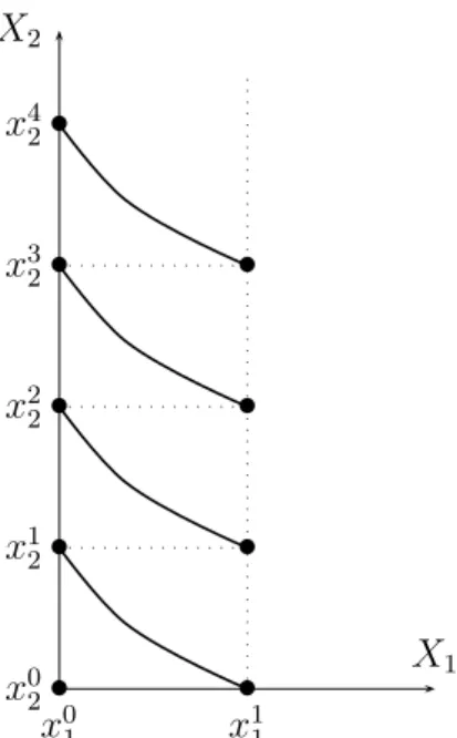
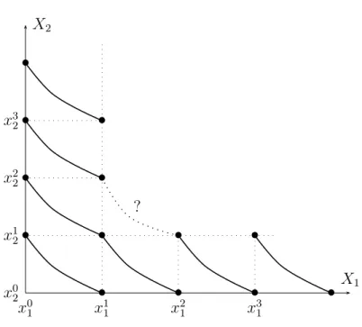
1, x11]). We may now proceed to build our standard sequence on the second attribute (see Figure 4) asking for levels x2 2, x32, . . . such that: (x0₁, x2₂) ∼ (x1₁, x1₂), (x0₁, x3₂) ∼ (x1₁, x2₂), . . . (x0₁, xk₂) ∼ (x1₁, xk−1₂ ). As above, using (2) leads to:

v2(x22) − v2(x12) = v1(x11) − v1(x01), v2(x32) − v2(x22) = v1(x11) − v1(x01), . . . v2(xk2) − v2(xk−12 ) = v1(x11) − v1(x01), so that: v2(x22) = 2, v2(x32) = 3, . . . , v2(xk2) = k.

This process of building a standard sequence of the second attribute therefore leads to defining v2 on a number of, carefully, selected elements of X2.

Remember the standard sequence that we built for length in section 1.2. An implicit hypothesis was that the length of any rod could be exceeded by the length of a composite object obtained by concatenating a sufficient number of perfect copies of a standard rod. Such an hypothesis is called “Archimedean” since it mimics the property of the real numbers saying that

x0 1 x0 2 X1 X2 x1 1 x1 2 x2 2 x3 2 x4 2 • • • • • • • • •

Figure 4: Building a standard sequence on X2.

for any positive real numbers x, y it is true that nx > y for some integer n, i.e. y, no matter how large, may always be exceeded by taking any x, no matter how small, and adding it with itself and repeating the operation a sufficient number of times. Clearly, we will need a similar hypothesis here. Failing it, there might exist a level y2 ∈ X2 that will never be “reached” by our standard sequence, i.e. such that y2 Â2 xk2, for k = 1, 2, . . .. For measurement models in which this Archimedean condition is omitted, see [139, 176].

Remark 13

At this point a good exercise for the reader is to figure out how we may extend the standard sequence to cover levels of X2 that are “below” the reference level x0

2. This should not be difficult. •

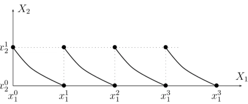
Now that a standard sequence is built on the second attribute, we may use any part of it to build a standard sequence on the first attribute. This will require finding levels x21, x31, . . . ∈ X1 such that (see Figure 5):

(x21, x02) ∼ (x11, x12), (x3₁, x0₂) ∼ (x2₁, x1₂),

. . .

x0 1 x0 2 X1 X2 x1 1 x21 x31 x31 x1 2• • • • • • • •

Figure 5: Building a standard sequence on X1.

Using (2) leads to:

v1(x21) − v1(x11) = v2(x12) − v2(x02), v1(x31) − v1(x21) = v2(x12) − v2(x02), . . . v1(xk1) − v1(xk−11 ) = v2(x12) − v2(x02), so that: v1(x21) = 2, v1(x31) = 3, . . . , v1(xk2) = k.

As was the case for the second attribute, the construction of such a sequence will require the structure of X1 to be adequately rich, which calls for a solv-ability assumption. An Archimedean condition will also be needed in order to be sure that all levels of X1 can be reached by the sequence.

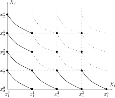
We have now defined a “grid” in X (see Figure 6) and we have v1(xk1) = k and v2(xk2) = k for all elements of this grid. Intuitively such numerical assignments seem to define an adequate additive value function on the grid. We have to prove that this intuition is correct. Let us first verify that:

α + β = γ + δ = ² ⇒ (xα₁, xβ₂) ∼ (xγ₁, xδ₂). (5) When ² = 1, (5) holds by construction because we have: (x0

1, x12) ∼ (x11, x02). When ² = 2, we know that (x01, x22) ∼ (x11, x12) and (x21, x02) ∼ (x11, x12) and the claim is proved using the transitivity of ∼.

Consider now the ² = 3 case. We have (x0

1, x32) ∼ (x11, x22) and (x01, x32) ∼ (x11, x22). It remains to be shown that (x21, x12) ∼ (x11, x22) (see the dotted arc in Figure 6). This does not seem to follow from the previous conditions that we more or less explicitly used: transitivity, independence, “richness”, Archime-dean. Indeed, it does not. Hence, we have to suppose that: (x2

x0 1 x0 2 X1 X2 x1 1 x21 x31 x1 2 x2 2 x3 2 • • • • • • • • • • • • • ?

Figure 6: The grid.

and (x0

1, x12) ∼ (x11, x02) imply (x21, x12) ∼ (x11, x22). This condition, called the Thomsen condition, is clearly necessary for (2). The above reasoning now easily extends to all points on the grid, using weak ordering, independence and the Thomsen condition. Hence, (5) holds on the grid.

It remains to show that:

² = α + β > ²0 = γ + δ ⇒ (xα₁, xβ₂) Â (xγ₁, xδ₂). (6) Using transitivity, it is sufficient to show that (6) holds when ² = ²0 _{+ 1.} By construction, we know that (x1

1, x02) Â (x01, x02). Using independence this implies that (x11, xk2) Â (x01, xk2). Using (5) we have (x11, xk2) ∼ (xk+11 , x02) and (x0

1, xk2) ∼ (xk1, x02). Therefore we have (xk+11 , x02) Â (xk1, x02), the desired conclusion.

Hence, we have built an additive value function of a suitably chosen grid (see Figure 7). The logic of the assessment procedure is then to assess more and more points somehow considering more finely grained standard sequences. The two techniques evoked for length may be used here depend-ing on the underlydepend-ing structure of X. A limitdepend-ing process then unambiguously defines the functions v1 and v2. Clearly such v1 and v2 are intimately related. Once we have chosen an arbitrary reference point (x01, x02) and a level x11 defin-ing the unit of measurement, the process just described entirely defines v1 and v2. It follows that the only possible transformations that can be applied to v1 and v2 is to multiply both by the same positive number α and to add

x0 1 x0 2 X1 X2 x1 1 x21 x31 x41 x1 2 x2 2 x3 2 x42 • • • • • • • • • • • • • • • • •

Figure 7: The entire grid.

to both a, possibly different, constant. This is usually summarized saying that v1 and v2 define interval scale with a common unit.

The above reasoning is a very rough sketch of the proof of the existence of an additive value function when n = 2, as well as a sketch of how it could be assessed. Careful readers will want to refer to [52, 115, 193].

Remark 14

As was already the case with the even swap technique, it is worth emphasiz-ing that this assessment technique makes no use of the vague notion of the “importance” of the various attributes. The “importance” is captured here in the lengths of the preference intervals on the various attributes.

A common but critical mistake is to confuse the additive value function model (2) with a weighted average and to try to assess weights asking whether an attribute is “more important” than another. This makes no sense. • Remark 15

The measurement of length through standard sequences envisaged above leads to a scale that is unique once the unit of measurement is chosen. At this point, a good exercise for the reader is to find an intuitive explanation to the fact that, when measuring the “length” of preference intervals, the origin of measurement becomes arbitrary. The analogy with the the measurement

of duration on the one hand and dates, as given in a calendar, on the other

hand should help. •

3.1.2 The case of more than two attributes

The good news now is that the process is exactly the same when there are more than two attributes. With one surprise: the Thomsen condition is no more needed to prove that the standard sequences defined on each attribute lead to an adequate value function on the grid. A heuristic explanation of this strange result is that, when n = 2, there is no difference between in-dependence and weak inin-dependence. This is no more true when n ≥ 3 and assuming independence is much stronger than just assuming weak indepen-dence.

3.2

Statement of results

We use below the “algebraic approach” [113, 115, 127]. A more restrictive approach using a topological structure on X is given in [41, 193]. We for-malize below the conditions informally introduced in the preceding section. The reader not interested in the precise statement of the results or, better, having already written down his own statement, may skip this section. Definition 16 (Thomsen condition)

Let % be a binary relation on a set X = X1 × X2. It is said to satisfy the Thomsen condition if

(x1, x2) ∼ (y1, y2) and (y1, z2) ∼ (z1, x2) ⇒ (x1, z2) ∼ (z1, y2), for all x1, y1, z1 ∈ X1 and all x2, y2, z2 ∈ X2.

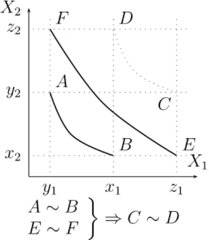
Figure 8 shows how the Thomsen condition uses two “indifference curves” to place a constraint on a third one. This was needed above to prove that an additive value function existed on our grid. Remember that the Thomsen condition is only needed when n = 2; hence, we only stated it in this case. Definition 17 (Standard sequences)

A standard sequence on attribute i ∈ N is a set {ak

i : aki ∈ Xi, k ∈ K} where K is a set of consecutive integers (positive or negative, finite or infinite) such that there are x−i, y−i ∈ X−i satisfying N ot[ x−i ∼−i y−i] and (aki, x−i) ∼ (ak+1_i , y−i), for all k ∈ K.

A standard sequence on attribute i ∈ N is said to be strictly bounded if there are bi, ci ∈ Xi such that bi Âi aki Âi ci, for all k ∈ K. It is then clear

X2 X1 y1 x1 z1 x2 y2 z2 A B C D E F A ∼ B E ∼ F ¾ ⇒ C ∼ D

Figure 8: The Thomsen condition.

that, when model (2) holds, any strictly bounded standard sequence must be finite.

Definition 18 (Archimedean)

For all i ∈ N , any strictly bounded standard sequence on i ∈ N is finite. The following condition rules out the case in which a standard sequence cannot be built because all levels are indifferent.

Definition 19 (Essentiality)

Let % be a binary relation on a set X = X1× X2× · · · × Xn. Attribute i ∈ N is said to be essential if (xi, a−i) Â (yi, a−i), for some xi, yi ∈ Xi and some a−i∈ X−i.

Definition 20 (Restricted Solvability)

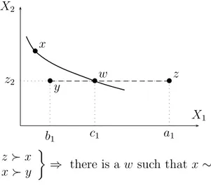
Let % be a binary relation on a set X = X1 × X2 × · · · × Xn. Restricted solvability is said to hold with respect to attribute i ∈ N if, for all x ∈ X, all z−i ∈ X−i and all ai, bi ∈ Xi, [(ai, z−i) % x % (bi, z−i)] ⇒ [x ∼ (ci, z−i), for some ci ∈ Xi].

Remark 21

Restricted solvability is illustrated in Figure 9 in the case where n = 2. It says that, given any x ∈ X, if it is possible find two levels ai, bi ∈ Xi such that when combined with a certain level z−i ∈ X−i on the other attributes, (ai, z−i) is above x and (bi, z−i) is below x, it should be possible to find a level ci, “in between” ai and bi, such that such that (ci, z−i) is exactly indifferent to x.

A much stronger hypothesis is unrestricted solvability asserting that for all x ∈ X and all z−i ∈ X−i, x ∼ (ci, z−i), for some ci ∈ Xi. Its use leads however to much simpler proofs.

It is easy to imagine situations in which restricted solvability might hold while unrestricted solvability would fail. Suppose, e.g. that a firm has to choose between several investment projects, two attributes being the Net Present Value (NPV) of the projects and their impact on the image of the firm in the public. Consider a project consisting in investing in the software market. It has a reasonable NPV and no adverse consequences on the image of the firm. Consider now another project that could have dramatic conse-quences on the image of the firm, because it leads to investing the market of cocaine. Unrestricted solvability would require that by sufficiently increas-ing the NPV of the second project it would become indifferent to the more standard project of investing in the software market. This is not required by

restricted solvability. • X1 X2 x • z2 b1 c1 a1 w •_y • •z z  x x  y ¾

⇒ there is a w such that x ∼ w

Figure 9: Restricted Solvability on X1.

We are now in position to state the central results concerning model (2). Proofs may be found in [115, 194].

Theorem 22 (Additive utility when n = 2)

Let % be a binary relation on a set X = X1×X2. If restricted solvability holds on all attributes and each attribute is essential then % has a representation in model (2) if and only if % is an independent weak order satisfying the Thomsen and the Archimedean conditions

Furthermore in this representation, v1 and v2 define an interval scale with a common unit, i.e. if v1, v2 and w1, w2 are two pairs of functions satisfying (2), there are real numbers α, β1, β2 with α > 0 such that, for all x1 ∈ X1 and all x2 ∈ X2

v1(x1) = αw1(x1) + β1 and v2(x2) = αw2(x2) + β2

When n ≥ 3 and at least three attributes are essential, the above result simplifies in that the Thomsen condition can now be omitted.

Theorem 23 (Additive utility when n ≥ 3)

Let % be a binary relation on a set X = X1 × X2 × . . . Xn with n ≥ 3. If restricted solvability holds on all attributes and at least 3 attributes are essential then % has a representation in model (2) if and only if % is an independent weak order satisfying the Archimedean condition.

Furthermore this representation defines an interval scale with a common unit.

Remark 24

As mentioned in introduction, the additive value model is central to several fields in decision theory. It is therefore not surprising that much energy has been devoted to analyze variants and refinements of the above results. Among the most significant ones, let us mention:

• the study of cases in which solvability holds only on some or none of the attributes [76, 77, 78, 138],

• the study of the relation between the “algebraic approach” introduced above and the topological one used in [41], see e.g. [102, 110, 193, 194]. The above results are only valid when X is the entire Cartesian product of the sets Xi. Results in which X is a subset of the whole Cartesian product X1 × X2 × . . . × Xn are not easy to obtain, see [34, 164] (the situation is “easier” in the special case of homogeneous product sets, see [195, 196]). •

3.3

Implementation: Standard sequences and beyond

We have already shown above how additive value functions can be assessed using the standard sequence technique. It is worth recalling here some of the characteristics of this assessment procedure:

• It requires the set Xi to be rich so that it is possible to find a preference interval on Xi that will exactly match a preference interval on another attribute. This excludes using such an assessment procedure when some of the sets Xi are discrete.

• It relies on indifference judgements which, a priori, are less firmly es-tablished than preference judgements.

• It relies on judgements concerning fictitious alternatives which, a priori, are harder to conceive than judgements concerning real alternatives. • The various assessments are thoroughly intertwined and, e.g., an

im-precision on the assessment of x1

2, i.e. the endpoint of the first interval in the standard sequence on X2 (see Figure 4) will propagate to many assessed values.

The assessment procedure based on standard sequences is therefore rather demanding; this should be no surprise given the proximity between this form of measurement and extensive measurement illustrated above on the case of length. Hence, the assessment procedure based on standard sequences seems to be seldom used in the practice of decision analysis [108, 191].

Many other simplified assessment procedures have been proposed that are less firmly grounded in theory. In many of them, the assessment of the partial value functions vi relies on direct comparison of preference differences without recourse to an interval on another attribute used as a “meter stick”. We refer to [45] for a theoretical analysis of these techniques. They are also studied in detail in Chapter XX of this volume (Chapter 6, Dyer).

These procedures include:

• direct rating techniques in which values of vi are directly assessed with reference to two arbitrarily chosen points [47, 48],

• procedures based on bisection, the decision-maker being asked to assess a point that is “half way” in terms of preference two reference points, • procedures trying to build standard sequences on each attribute in

terms of “preference differences” [115, ch. 4].

4

The additive value model in the “finite”

case

4.1

Outline of Theory

We suppose in this section that % is a binary relation on a finite set X ⊆ X1 × X2 × · · · × Xn (contrary to the preceding section, dealing with sub-sets of product sub-sets will raise no difficulty here). The finiteness hypothesis clearly invalidates the standard sequence mechanism used till now. On each attribute there will only be finitely many “preference intervals” and exact matches between preference intervals will only happen exceptionally.

Clearly, independence remains a necessary condition for model (2) as before. Given the absence of structure of the set X, it is unlikely that this condition is sufficient to ensure (2). The following example shows that this intuition is indeed correct.

Example 25

Let X = X1× X2 with X1 = {a, b, c} and X2 = {d, e, f }. Consider the weak order on X such that, abusing notation in an obvious way,

ad  bd  ae  af  be  cd  ce  bf  cf.

It is easy to check that % is independent. Indeed, we may for instance check that:

ad  bd and ae  be and af  bf, ad  ae and bd  be and cd  ce.

This relation cannot however be represented in model (2) since: af  be ⇒ v1(a) + v2(f ) > v1(b) + v2(e),

be  cd ⇒ v1(b) + v2(e) > v1(c) + v2(d), ce  bf ⇒ v1(c) + v2(e) > v1(b) + v2(f ), bd  ae ⇒ v1(b) + v2(d) > v1(a) + v2(e). Summing the first two inequalities leads to:

v1(a) + v2(f ) > v1(c) + v2(d). Summing the last two inequalities leads to:

a contradiction.

Note that, since no indifference is involved, the Thomsen condition is trivially satisfied. Although it is clearly necessary for model (2), adding it to

independence will therefore not solve the problem. 3

The conditions allowing to build an additive utility model in the finite case were investigated in [1, 2, 162]. Although the resulting conditions turn out to be complex, the underlying idea is quite simple. It amounts to finding conditions under which a system of linear inequalities has a solution.

Suppose that x  y. If model (2) holds, this implies that: n X i=1 vi(xi) > n X i=1 vi(yi). (7) Similarly if x ∼ y, we obtain: n X i=1 vi(xi) = n X i=1 vi(yi). (8)

The problem is then to find condition on % such that the system of finitely many equalities and inequalities (7-8) has a solution. This is a classical problem in Linear Algebra [74].

Definition 26 (Relation Em )

Let x1_{, x}2_{, . . . , x}m_{, y}1_{, y}2_{, . . . , y}m _{∈ X. We say that} (x1_{, x}2_{, . . . , x}m_)Em_(y1_{, y}2_{, . . . , y}m₎ if, for all i ∈ N , (x1

i, x2i, . . . , xmi ) is a permutation of (yi1, yi2, . . . , yim).

Suppose that (x1_{, x}2_{, . . . , x}m_)Em_(y1_{, y}2_{, . . . , y}m_{) then model (2) implies} that m X j=1 n X i=1 vi(xji) = m X j=1 n X i=1 vi(yij).

Therefore if xj _%yj _{for j = 1, 2, . . . , m − 1, it cannot be true that x}m _{Â y}m_. This condition must hold for all m = 2, 3, . . ..

Definition 27 (Condition Cm ) We say that condition Cm _{holds if}

[xj _%yj _{for j = 1, 2, . . . , m − 1] ⇒ N ot[ x}m _{Â y}m_] for all x1_{, x}2_{, . . . , x}m_{, y}1_{, y}2_{, . . . , y}m _{∈ X such that}

Remark 28

It is not difficult to check that: • Cm+1 ⇒ Cm,

• C2 _{⇒ % is independent,}

• C3 _{⇒ % is transitive. •}

We already observed that Cm _{was implied by the existence of an additive} representation. The main result for the finite case states that requiring that % is complete and that Cm _{holds for m = 2, 3, . . . is also sufficient. Proofs} can be found in [52, 115].

Theorem 29

Let % be a binary relation on a finite set X ⊆ X1× X2× · · · × Xn. There are real-valued functions vi on Xi such that (2) holds if and only if % is complete and satisfies Cm _{for m = 2, 3, . . ..}

Remark 30

Contrary to the “rich” case envisaged in the preceding section, we have here necessary and sufficient conditions for the additive value model (2). However, it is important to notice that the above result uses a denumerable scheme of conditions. It is shown in [163] that this denumerable scheme cannot be truncated: for all m ≥ 2, there is a relation % on a finite set X such that Cm holds but violating Cm+1_{. This is studied in more detail in [125, 183, 199].} Therefore, no finite scheme of axioms is sufficient to characterize model (2) for all finite sets X.

Given a finite set X of given cardinality, it is well-known that the denu-merable scheme of condition can be truncated. The precise relation between the cardinality of X and the number of conditions needed raises difficult combinatorial questions that are studied in [70, 71]. • Remark 31

It is clear that, if a relation % has a representation in model (2) with functions vi, it also has a representation using functions v0i = αvi + βi with α > 0. Contrary to the rich case, the uniqueness of the functions vi is more complex as shown by the following example.

Example 32

Let X = X1 × X2 with X1 = {a, b, c} and X1 = {d, e}. Consider the weak order on X such that, abusing notation in an obvious way,

This relation has a representation in model (2) with

v1(a) = 3, v1(b) = 1, v1(c) = 0, v2(d) = 3, v2(e) = 0.5.

An equally valid representation would be given taking v1(b) = 2. Clearly this new representation cannot be deduced from the original one applying a

positive affine transformation. 3

Remark 33

Theorem 29 has been extended to the case of an arbitrary set X in [100]. The resulting conditions are however quite complex. This explains why we spent time on this “rich” case in the preceding section. • Remark 34

The use of a denumerable scheme of conditions in theorem 29 does not fa-cilitate the interpretation and the test of conditions. However it should be noticed that, on a given set X, the test of the Cm _{conditions amounts to} finding if a system of finitely many linear inequalities has a solution. It is well-known that Linear Programming techniques are quite efficient for such

a task. •

4.2

Implementation: LP-based assessment

We show how to use LP techniques in order to assess an additive value model (2), without supposing that the sets Xi are rich. For practical purposes, it is not restrictive to assume that we are only interested in assessing a model for a limited range on each Xi. We therefore assume that the sets Xi are bounded so that, using independence, there is a worst value xi∗ and a most preferable value x∗

i. Using the uniqueness properties of model (2), we may always suppose, after an appropriate normalization, that:

v1(x1∗) = v2(x2∗) = . . . = vn(xn∗) = 0 and (9) n

X

i=1

vi(x∗i) = 1. (10)

Two main cases arise (see Figures 10 and 11):

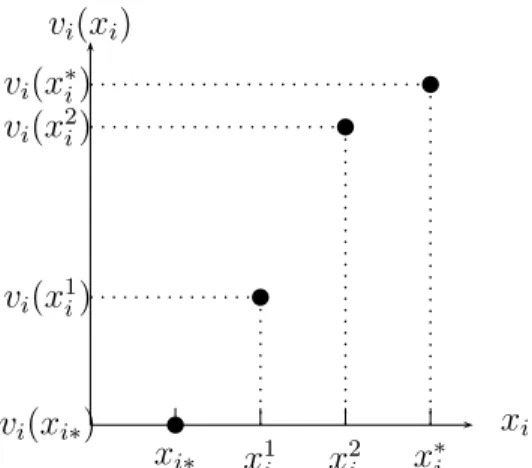
• attribute i ∈ N is discrete so that the evaluation of any conceivable alternative on this attribute belongs to a finite set. We suppose that Xi = {xi∗, x1i, x2i, . . . , x

ri

i , x∗i}. We therefore have to assess ri+ 1 values of vi,

vi(xi) xi xi∗ x1_i x2_i x∗_i vi(xi∗) vi(x1i) vi(x2i) vi(x∗i)

Figure 10: Value function when Xi is discrete. vi(xi) xi xi∗ x1_i x2_i x3_i x∗_i vi(xi∗) vi(x1i) vi(x2i) vi(x3i) vi(x∗i)

Figure 11: Value function when Xi is continuous.

• the attribute i ∈ N has an underlying continuous structure. It is hardly restrictive in practice to suppose that Xi ⊂ R, so that the evaluation of an alternative on this attribute may take any value between xi∗ and x∗

i. In this case, we may opt for the assessment of a piecewise linear approximation of vi partitioning the set Xi in ri+ 1 intervals and supposing that vi is linear on each of these intervals. Note that the approximation of vi can be made more precise simply by increasing the number of these intervals.

With these conventions, the assessment of the model (2) amounts to giving a value to Pn

i=1(ri+ 1) unknowns. Clearly any judgment of preference linking x and y translate into a linear inequality between these unknowns. Similarly any judgment of indifference linking x and y translate into a linear equality. Linear Programming (LP) offers a powerful tool for testing whether such a

system has solutions. Therefore, an assessment procedure can be conceived on the following basis:

• obtain judgments in terms of preference or indifference linking several alternatives in X,

• convert these judgments into linear (in)equalities, • test, using LP, whether this system has a solution.

If the system has no solution then one may envisage either to propose a so-lution that will be “as close as possible” from the information obtained, e.g. violating the minimum number of (in)equalities or to suggest the reconsid-eration of certain judgements. If the system has a solution, one may explore the set of all solutions to this system since they are all candidates for the establishment of model (2). These various techniques depend on:

• the choice of the alternatives in X that are compared: they may be real or fictitious, they may differ on a different number of attributes, • the way to deal with the inconsistency of the system and to eventually

propose some judgments to be reconsidered,

• the way to explore the set of solutions of the system and to use this set as the basis for deriving a prescription.

Linear programming offers of simple and versatile technique to assess additive value functions. All restrictions generating linear constraints of the coefficient of the value function can easily be accommodated. This idea has been often exploited, see [15]. We present below two techniques using it. It should be noticed that rather different techniques have been proposed in the literature on Marketing [32, 92, 93, 101, 118].

4.2.1 UTA [99]

UTA (“UTilit´e Additive”, i.e. additive utility in French) is one of the oldest technique belonging to this family. It is supposed in UTA that there is a subset Ref ⊂ X of reference alternatives that the decision-maker knows well either because he/she has experienced them or because they have received particular attention. The technique amounts to asking the DM to provide a weak order on Ref . Each preference or indifference relation contained in this weak order is then translated into a linear constraint: