HAL Id: tel-01012222
https://tel.archives-ouvertes.fr/tel-01012222
Submitted on 25 Jun 2014
HAL is a multi-disciplinary open access
archive for the deposit and dissemination of sci-entific research documents, whether they are
pub-L’archive ouverte pluridisciplinaire HAL, est destinée au dépôt et à la diffusion de documents scientifiques de niveau recherche, publiés ou non,
architectures in bioinformatics : applications to genetics,
structure comparison and large graph analysis
Guillaume Chapuis
To cite this version:
Guillaume Chapuis. Exploiting parallel features of modern computer architectures in bioinformatics : applications to genetics, structure comparison and large graph analysis. Bioinformatics [q-bio.QM]. École normale supérieure de Cachan - ENS Cachan, 2013. English. �NNT : 2013DENS0068�. �tel-01012222�
THÈSE / ENS CACHAN - BRETAGNE
sous le sceau de l’Université européenne de Bretagne
pour obtenir le titre de
DOCTEUR DE L’ÉCOLE NORMALE SUPÉRIEURE DE CACHAN
Mention : Informatique
École doctorale MATISSE
présentée par
Guillaume Chapuis
Préparée à l’Unité Mixte de Recherche 6074 Institut de recherche en informatique et systèmes aléatoires / Inria Rennes
Exploiting parallel
features of modern
computer architectures in
bioinformatics
Applications to genetics, structure comparisonThèse soutenue le 18 décembre 2013
devant le jury composé de :
Nouredine Melab Professeur / rapporteur Gunnar Klau Professeur / rapporteur Frédéric Guinand Professeur / examinateur Patrice Quinton Professeur / examinateur
Contents
1 Introduction 7
2 Background 11
2.1 Introduction . . . 11
2.2 Overview of CPU and GPU architectures . . . 12
2.3 Hierarchy of computational problems . . . 13
2.4 Coarse-grain parallelism . . . 14
2.4.1 Multicore CPU programming . . . 15
2.4.2 GPU programming . . . 17 2.5 Fine-grain parallelism . . . 21 2.5.1 Vector instructions . . . 22 2.5.2 Bit-level parallelism . . . 23 2.5.3 Instruction-level parallelism . . . 23 2.6 Parallelization in bioinformatics . . . 23 2.6.1 Sequence comparison . . . 24 2.6.2 Structure comparison . . . 26 2.7 Conclusion . . . 28
3 GPU accelerated QTL mapping 29 3.1 Introduction to QTL mapping . . . 29
3.2 Methods and algorithms . . . 32
3.2.1 Linkage Analysis . . . 32
3.2.2 Linkage Disequilibrium and LDL Analyses . . . 33
3.2.3 Thresholds detection . . . 33
3.2.4 Algorithms for QTL detection . . . 34
3.3 GPU implementation . . . 36
3.3.1 Mapping computations on the GPU . . . 37
3.3.2 Optimizing GPU memory usage . . . 38
3.3.3 Reducing CPU/GPU transfers . . . 39
3.3.4 Optimizing homoskedastic analyses . . . 39
3.4 Experiments and results . . . 40
3.4.1 Execution times . . . 40
3.4.2 Speedups . . . 41
3.5 Conclusion . . . 43 4 Efficient Multi-GPU Computation of All-Pairs Shortest Paths 47
4.1 Introduction . . . 47
4.2 Related Work . . . 50
4.3 Algorithm details . . . 51
4.3.1 Overview . . . 52
4.3.2 Step 1: Graph decomposition . . . 52
4.3.3 Step 2: Computing distances within each graph component . . 52
4.3.4 Step 3: Computing distances in the boundary graph . . . 54
4.3.5 Step 4: Distances between non-boundary vertices . . . 55
4.4 Implementation . . . 57
4.4.1 Data organization . . . 57
4.4.2 Work analysis . . . 59
4.4.3 Parallel implementation . . . 61
4.4.4 Memory limitations . . . 62
4.5 Results and perspectives . . . 62
5 Parallel seed-based approach to protein structure similarity detection 67 5.1 Introduction . . . 67
5.1.1 Alignment graphs . . . 68
5.1.2 Relation to protein structure comparison . . . 69
5.1.3 Measures for protein alignments . . . 69
5.2 Methods . . . 70
5.2.1 Our approach . . . 70
5.2.2 Overview of the algorithm . . . 70
5.2.3 Seed enumeration . . . 71
5.2.4 Seed extension . . . 72
5.2.5 Extension filtering . . . 73
5.2.6 Guarantees on resulting alignments’ RM SD scores . . . 74
5.2.7 Result ranking . . . 75
5.2.8 k-to-k alignments . . . 76
5.2.9 Graph splitting . . . 77
5.3 Parallelism . . . 78
5.3.1 Overview of the implemented parallelism . . . 78
5.3.2 Coarse-grain parallelism . . . 78
5.3.3 Fine-grain parallelism . . . 80
5.4 Results and perspectives . . . 81
6 Conclusions and perspectives 85 6.1 Conclusions . . . 85
6.2 Perspectives . . . 86
6.2.1 QTL detection . . . 86
6.2.2 Large graph analysis . . . 86
6.2.3 Protein structure comparison . . . 87
6.2.4 General remarks . . . 87
List of Figures
2.3.1 Rough classification of computational problems from a parallelism
point of view. . . 15
2.5.1 Differences between scalar and vector instructions. . . 22
2.5.2 Bit parallel set intersection. . . 23
2.5.3 Example of data dependencies. . . 24
3.1.1 Repartition of markers M1/M2 and N1/N2 on alleles Q1 and Q2. . . 30
3.2.1 Description of a contingency matrix used for computations at each genome position and for each simulation. . . 36
3.3.1 Example of gridification on the GPU. . . 37
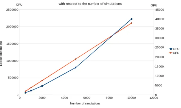
3.4.1 Evolution of the execution time with respect to the number of simu-lations. . . 41
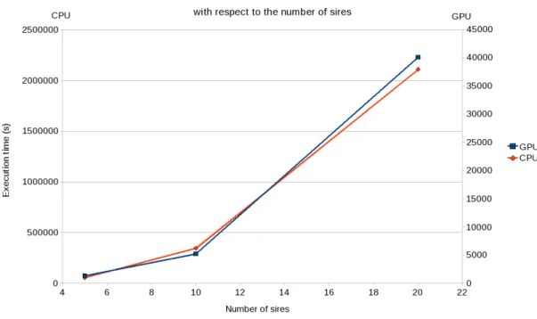
3.4.2 Evolution of the execution time with respect to the number of half-sib families. . . 42
3.4.3 Evolution of the execution time with respect to the number of genome positions. . . 42
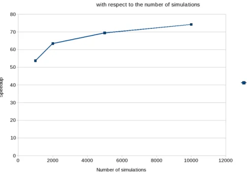
3.4.4 Speedup with respect to the number of simulations. . . 43
3.4.5 Speedup with respect to the number of half-sib families. . . 44
3.4.6 Speedup with respect to the number of genome positions. . . 44
4.3.1 Illustration to the proof of Lemma Theorem 1. The shaded region illustrates a component C with the subpath q = (xbi, xbi+1, . . . , xbi+1) of p inside it. . . 55
4.3.2 Illustration to the proof of Lemma Theorem 2. Note that while in the figure both vi and vj are non-boundary, the proof does not make such an assumption. . . 57
4.4.1 Adjacency matrix after reordering of the vertices. Vertices from the same component are stored contiguously starting with boundary ver-tices (in red). . . 58
4.4.2 The boundary matrix, here in red, is scattered over the adjacency matrix. Step 3 consits in reconstituting the boundary matrix and computing shortest distances. . . 59
4.4.3 Computations associated to each non-diagonal sub-matrix uses data from 2 diagonal sub-matrices and part of the non-diagonal sub-matrix itself. Computations are similar to matrix multiplications. . . 60
4.5.1 Evolution of run times with respect to the number of vertices. Two implementations are compared: our implementation using external memory and the GPU Dijkstra implementation from [OATLGE13]. Computations were run using two GPUs on a single cluster node. . . 63 4.5.2 Evolution of speedups with respect to the number of GPUs. The ideal
scaling line is given as a reference. . . 64 4.5.3 Evolution of run times with respect to the number of vertices. Three
implementations are compared: our two implementations - with and without using external memory - and a distributed Dijkstra imple-mentation referred to as CPU Dijkstra. All computations were run on 64 cluster nodes. . . 65 5.1.1 Example of an alignment graph used here to compare the structures
of two proteins. The presence of an edge between vertex (1, 1) and vertex (3, 2) means that the distance between atoms 1 and 2 of protein 1 is similar to the distance between atoms 1 and 3 of protein 2. The clique (2, 1) (3, 2) (4, 3) indicates that RMSD of structures (2, 3, 4) and (1, 2, 3) is less than 2τ . . . 68 5.2.1 Example of symmetry issues. Even though, vertex vl = (L, L′)
be-longs to the extension of seed(vi, vj, vk), points L and L′ lie on
dif-ferent sides of the plane defined by optimally superimposed triangles
IJK and I′
J′
K′
. . . 73 5.2.2 Illustration of the guarantee on the similarity of internal distances
between two pairs of atoms vl = (L, L′) and vm = (M, M′), here
represented in yellow, added to a seed (vi, vj, vk) represented in blue.
Dashed lines represent internal distances, the similarity of which is tested in the alignment graph. . . 75 5.2.3 Example of 1-to-1 alignments retrieved from a k-to-k alignments. In
red, a 1-to-1 alignment of optimal length but sub-optimal RMSDc and in green a 1-to-1 alignment of optimal length and optimal RMSDc. Solving the assignment problem on this graph yields the green align-ment. . . 77 5.3.1 Overview of the implemented parallelism. . . 79 5.3.2 Bit vector representation of the neighbors of vertex vi in an alignment
graph G(V, E). In this example, vj unlike vk is a neighbor of vi. . . . 80
5.3.3 Intersection of neighbors of vertex vi and vertex vj. . . 81
5.4.1 These two proteins are both composed of two similar domains - named A and B for 4clna (left), and C and D for 2bbma (right). These domains are separated by a a flexible bridge. . . 82 5.4.2 Visualizations of the results for the comparison of proteins 4clna and
2bbma returned by CMO, PAUL and the four top alignments of our approach. . . 82 5.4.3 Evolution of run times with respect to # of edges in the alignment
List of Algorithms
3.1 Algorithm for heteroskedastic analysis . . . 35
3.2 Algorithm for homoskedastic analysis . . . 35
4.1 Floyd-Warshall algorithm. . . 49
4.2 Dijkstra’s Single Source Shortest Path algorithm. . . 49
4.3 Partitioned All-Pairs Shortest Path algorithm . . . 53
5.1 Overview of the algorithm . . . 71
5.2 Seed enumeration . . . 72
5.3 Seed extension . . . 73
5.4 Extension filtering algorithm . . . 74
List of Tables
3.2 Values and ranges of values for fixed and variable parameters used in Fig. 3.4.4, Fig. 3.4.5, and Fig. 3.4.6. . . 45 3.1 Values and ranges of values for fixed and variable parameters used in
Fig. 3.4.1, Fig. 3.4.2, and Fig. 3.4.3. . . 45 5.1 Details of the alignments returned by other tools - columns 2 through
4 - and our method - columns 5 through 8. Best scores are in italics. . 83 5.2 Run times and speedups for varying # of cores. . . 83
1 Introduction
The recently renewed interest in parallel computing stems from a conjunction of two very different factors. On the one hand, data generation in many fields is be-coming exponentially cheaper yielding a data tsunami and greatly increasing the demand for time-consuming computations. On the other hand, computer architec-tures are undergoing a drastic shift from exponentially increasing clock frequencies to exponentially increasing parallel capabilities.
The exponential growth of available data to process lead to the emergence of the concept of Big Data. Although the term was first used in 1941 according to the Oxford English Dictionary, it really became popular around the year 2007; a special issue of Nature in 2008 was even entirely dedicated to the Big Data concept [HCF+08, Lyn08, W+08]. Coping with the Big Data phenomenon poses several
challenges in terms of storage, search, sharing, analysis and transfers of the data. In this thesis, we will concentrate on the computational aspect of the challenges, ie. how to analyze large datasets using the limited capabilities of modern computers. From a computational point of view, large datasets require efficient implementation in order to reduce runtimes to a reasonable level as well as a careful usage of the limited main memory available on a given computer.
The simultaneity of the regain in popularity of the Big Data concept and the recent change in computer architectures may not be solely coincidental. The sudden halt in the evolution of processor clock frequencies drastically accentuated the challenges of Big Data, from a computational point of view at least. Before this shift in computer architectures, any program could process a larger amount of data by simply having it run on a newer computer with a higher clock frequency. Increasing the parallel capabilities of a computer will however have no immediate impact on a sequential program’s runtime. Parallel capabilities of modern computers require efforts from programmers to be fully exploited. Some computational problems will not even benefit from parallelism; others may be well suited for certain types of parallelism but will not be accelerated by other types. Implementing a parallel version of an algorithm must therefore be preceded by a careful analysis to exhibit parallelism and find suitable parallel hardware to target.
This conjunction of factors is particularly noticeable in bioinformatics. Recent advances in data generation such as High-Throughput Sequencing technologies have stressed the need for efficient implementations, fully exploiting parallel capabilities of modern computers, to handle the massive amount of data to process. The same phenomenon can be observed in other domains such as protein comparison and pro-tein interaction analyses, where propro-tein databases have known the same exponential growth. In the past few years, parallel implementations have flourished targeting
various parallel architectures such as multicore Central Processing Units (CPUs) and manycore Graphics Processing Units (GPUs).
This thesis focuses on exploiting the parallel capabilities of modern computers for computationally intensive bioinformatics problems. Various problems are studied, from which different types of parallelism can be exhibited and exploited.
Chapter 3 describes the various parallelism techniques that can be employed on a modern computer and the types of computational problems to which they can ben-efit. We then detail some recurring problems in bioinformatics that have previously been ported onto parallel hardware. Two types of parallelism are discussed here:
• Fine-grain parallelism, in which we include the use of CPU vector instructions and bit-level parallelism techniques;
• Coarser-grain parallelism such as multicore CPU implementations and many-core GPU implementations.
This distinction between fine- and coarse-grain parallelisms is of course arbitrary and depends on the application; GPU parallelism can be considered fine-grain parallelism in the context of a multinode cluster parallelization.
Chapter 4 proposes a GPU implementation of a tool for Quantitative Trait Locus (QTL) detection called QTLMap. The embarrassingly parallel structure of the statistical approach developed in QTLMap, makes it an ideal candidate for a porting to the GPU architecture. This new implementation is up to 75 times faster than the previous multicore CPU version. This speedup can however only in part be imputed to the use of a GPU. Some optimizations have been specifically made to accelerate the GPU implementation; these optimizations could also be implemented on the CPU version of the tool. Faster QTL analyses allow geneticists to consider more precise computations and the processing of larger datasets.
In chapter 5, we discuss a new algorithm for the All-Pairs Shortest Paths (APSP) problems. APSP consists in finding the minimum distance between any two vertices of a weighted graph. This new algorithm, derived from the Floyd-Warshall algo-rithm, targets graphs with good community properties and develops a partitioned approach to the problem. The two-level parallelism exhibited by this algorithm allow for a multi-node GPU implementation. Computations are intended on large clusters of multi-GPU nodes and thus for very large instances of the problem - graphs with up to 109 vertices. Computing the shortest distances between all pairs of vertices in
a graph is the first step to obtaining many graph measures that are useful in various domains. Large graph analysis becomes crucial in bioinformatics when studying large protein protein interaction networks for instance.
In chapter 6, we propose a new approach to protein structure comparison and its parallel implementation. This new algorithm was early on developed with paral-lelism in mind. The implementation exploits multiple levels of paralparal-lelism such as vector instructions, bit-level parallelism with a bit-parallel set representation and computations across multiple cores of a CPU. These multiple levels of parallelism allow a more in depth analysis of the similarities between two proteins by providing
Introduction
more than a single pair of similar regions to be returned as well as more compli-cated configurations to be taken into account, such as sequence inversions and local flexibility of proteins.
2 Background
2.1 Introduction
The aim of bioinformatics is to use state of the art techniques stemming from the computer science field to tackle computationally intensive biological problems. Bioinformatics embraces fields such as DNA or protein sequence alignments, anal-ysis and comparison of protein or RNA structures. All these fields have known an exponential increase in the amount of available data in the past decades.
DNA sequencing is perhaps the most striking example of this rapid increase in data availability. Sequencing techniques have dramatically improved since the first sequencing of an organism in 1977, a 5386 base-pair long bacteriophage [SNC77]. Sequencing of the human genome, more than 3 billion base-pairs, was achieved in the year 2000 at the steep price of several billion dollars. Nowadays, next generation sequencing technologies have drastically reduced the price down to about 7k dollars. The consequence of the decrease in price of data generation is an explosion in size of databases in many fields. This phenomenon, referred to as Big Data, has rendered traditional tools incapable of outputting results in a reasonable time frame. The Big Data phenomenon also poses serious issues in terms of storage. Simultaneously, microprocessor architecture are rapidly evolving in a completely new direction.
Up until around 2007, processor clock frequencies increased exponentially, dou-bling approximately every 2 years. This exponential growth then came to a halt due to the power wall. Sustaining increasing clock frequencies would come at the price of a prohibitively high power consumption. Microprocessor manufacturers however still manage to follow Moore’s Law, which states that the number of transistors on a single chip grows exponentially [M+65, Moo] - doubling approximately every 2 years
in practice. This increasing number of transistors does not however go towards in-creasing clock frequencies anymore but instead mostly towards more computational units on a single chip.
From a programmer’s point of view, an increase in the number of processing units is very different from an increase in clock frequency. Doubling the clock frequency means that the same sequential program will run effortlessly up to twice as fast. On the other hand, doubling the number of computational units will have absolutely no impact on the run time of the sequential program. In order to benefit from the additional computational units, one has to undergo the tedious process of paral-lelizing the sequential program. Not all programs, however, can benefit from this parallelizing process. With twice as many computational units available, run times of a parallel program will at most be reduced by a factor 2 but this ideal case is far
from being the norm.
Central Processing Units (CPU) have only recently adopted parallel architec-tures as a standard for even general public computers. Graphics Processing Units (GPUs) have had that approach for a little longer, which is why the computational capabilities of these components has increasingly drawn the attention of the high performance computing community. GPUs present a massively parallel architecture with an impressive theoretical computational throughput and are an integral part of most modern computers.
Taking advantage of all the computational power offered by a modern computer means using its CPU cores simultaneously as well as its GPUs. In terms of paral-lelism, modern CPUs also offer vector instructions allowing executions of the same instruction over multiple data simultaneously. These parallelizing techniques are however not suited for every problem. Deciding which approach to consider and implementing it for a particular problem requires a careful analysis of the problem to be solved.
In this chapter, we first describe the differences between the CPU and the GPU architectures. We then give an overview of the different types of existing compu-tational problems as well as some hints about which types of parallelism that can be considered. The following sections give an overview of the parallel capabilities offered by modern computers. We finally present recent examples of parallel appli-cations in bioinformatics.
2.2 Overview of CPU and GPU architectures
Central processing units (CPUs) and graphics processing units (GPUs) have very different architectures. These differences stem from the fact that these two compo-nents had very distinct original purposes. On the first hand, CPUs are designed to be all purpose processing units. CPUs must be able to run a variety of heteroge-neous programs and in particular an operating system. GPUs on the other hand, are components initially dedicated to image rendering. They were originally designed to compute the values of each pixel to display on the screen.
A typical computer screen displays millions of pixels that need to be refreshed dozens of times every second. The tasks associated to updating each of these pixels are almost always identical and independent - or solely depend on the values of other pixels in the near vicinity. GPU architecture was therefore designed to exploit the massive parallelism inherent to image rendering. In that regard, GPUs can nowadays be successfully used in general computations to solve problems that present the same properties as image rendering - i.e. problems that can be decomposed in a large number of independent tasks.
Modern CPUs are composed of several cores offering interesting parallel capabil-ities. These cores are fast, all-purpose processing units that benefit from a large cache hierarchy and a dedicated control unit. New technologies such as Intel’s Hyper-threading even allow each of these cores to run two threads at full speed
2.3 Hierarchy of computational problems
simultaneously. Each thread also has access to larger registers and an associated set of vector instructions. These instructions allow each core to perform multiple iden-tical instructions simultaneously over different data items. Due to their dedicated control units, two CPU cores of a single CPU can execute different instructions at the same time; this property allows multicore CPUs to run independent processes simultaneously.
Modern GPUs, on the other hand, are composed of a large number of multipro-cessors. Each multiprocessor has its own control unit and a small manual cache memory; both of them are shared among a large number of GPU cores. Recent GPUs also offer a small automatic cache shared among GPU cores of each multi-processor. The fact that the control unit is shared among GPU cores from the same multiprocessors forces these GPU cores to always execute the same instruction over different data items at all times. In this sense, GPU multiprocessors are very similar to a single CPU core only executing vector instructions.
With the increasing use of GPUs in general purpose computations, the need for more CPU-like features becomes greater. GPU vendors are adapting to this recent demand. This trend can be observed in the integration of more precise floating point units, conforming with IEEE standards; in the increasing set of available instructions or in the recent adding of l1 and l2 caches.
In the meantime, CPU vendors, limited by the power wall, cannot keep increasing processor frequencies as they used to until around the year 2007. CPU performances are however still improving, though not by increasing clock frequencies. Instead, better performances are obtained, for example, by issuing more instructions per clock cycle, a process referred to as instruction level parallelism (ILP), by increasing the size of SSE vectors and their related set of instructions or by increasing the number of CPU cores on a single chip. Thus, CPU performances nowadays mostly improve by the addition of parallel features at different levels.
Both the CPU and GPU architectures are slowly merging to a hybrid architecture exhibiting traits inherited from traditional CPUs, i.e. all-purposeness, and from GPUs, i.e. massive parallelism. However, as of today, clear distinctions between the two architectures remain and it is up to developers to determine which type of parallelism to exploit depending on the studied problem, and what architecture best suits their needs.
2.3 Hierarchy of computational problems
Having access to highly parallel hardware with modern CPUs and GPUs does not mean that any implementation of a computational problem can be significantly accelerated. Some computational problems are inherently sequential and will not benefit from an attempt at parallelizing them. A common analogy for such problems comes from the software development field and claimed that adding manpower to a late project makes it later. The analogy states that “nine women can’t make a baby in a month”.
This analogy is also valid in our case. Some problems simply do not benefit from additional computational units. Thus no attempt should be made at parallelizing such computational problems. An example of such an inherently sequential problem is optimally playing a card game; computing which card is the best to play at a given round always depends on the previously played cards, thus one cannot compute rounds n and n + 1 simultaneously. However computing a single round may be breakable into independent tasks.
In order to be consider parallel, a computational problem should be breakable into independent tasks. Two tasks are considered independent if one does not need the result of the other to be computed. These independent tasks can then be computed independently and simultaneously on different processing units. Being able to break down a problem into independent task does not however ensure that a parallelization attempt will yield a decent speedup. If said tasks are greatly unbalanced for instance, balancing the total workload between the available processing may become tricky or even impossible. If, for example, one task represents 90 percent of the total execution time, any effort at balancing the workload is vain.
A computational problem is considered embarrassingly parallel if it is parallel and if all the sub-tasks composing the problem are perfectly balanced and identical. This strong property makes load balancing between the computational units trivial. Problems exhibiting this property are also candidates for executions on hardware that require that identical operations are computed between different computing units at all times. Such hardware include vector instructions on a CPU and GPU multiprocessors.
Figure Fig. 2.3.1 shows a rough classification of computational problems. Belong-ing to a given class of problem gives hints into which type of hardware is best for a given problem but is not nearly enough to make a decision. Many other aspects of the problem must also be taken into account to decide whether it fully complies with specific hardware restrictions. Such aspects include memory access patterns, number of independent tasks or required memory.
2.4 Coarse-grain parallelism
Parallelism can be exploited at many different hardware levels in today’s comput-ers. Parallelism can range from distributing computations over a grid to executing two instructions simultaneously on a single computation unit. The former type of parallelism is considered coarse grain parallelism, while the latter is considered fine grain parallelism. The grain traditionally refers to the size of the tasks that are run in parallel. When distributing computations over a grid, the overhead induced by the communication between nodes is far from negligible and, in order to better amortize it, the initial problem must be split into large tasks; therefore, parallelism over a grid of computers is considered coarse grain.
In this chapter, we focus on parallelism on a single machine. What we will consider coarse grain parallelism here is using multiple cores of a modern CPU and offsetting
2.4 Coarse-grain parallelism Computational problems Task parallel problems Embarrassingly parallel problems Inherently sequential problems Parallel problems
Figure 2.3.1: Rough classification of computational problems from a parallelism point of view.
computations to a GPU. In these two cases also, substantial speedups can only be obtained when tasks are large enough. When programming on a multicore CPU, the size of the tasks needs to amortize the overhead induced by spawning multiple threads and in the case of GPU programming it needs to amortize the overhead induced by the communications between the CPU and the GPU.
2.4.1 Multicore CPU programming
Most modern general public CPUs are multicore. In order to make full use of a recent CPU, a program must exploit the computational power of all CPU cores simultaneously. Each CPU core can be seen as an independent CPU in the sense that very different tasks can be assigned simultaneously to two different cores. This form of coarse-grain parallelism is referred to as MIMD (for Multiple Instructions Multiple Data); at any moment, two cores can be executing different instructions over different pieces of data.
CPU cores share the same memory. Shared memory has the advantage of allow-ing easy communication between cores but leaves to the programmer the tedious responsibility of ensuring data consistency. In order to prevent two or more cores from modifying the same memory address concurrently, complex mechanisms must be implemented. Various strategies exist to do so and depend on the framework chosen by the programmer. Two multicore frameworks are exposed in this section:
programming;
• The OpenMP interface, a higher-level approach. 2.4.1.1 The POSIX threads library
The POSIX threads library is a standardized C language threads programming in-terface for UNIX systems that was specified by the IEEE POSIX 1003.1c standard in 1995. This standard programming interface emerged to provide a cross-platform alternative to already existing proprietary APIs proposed by hardware vendors. Nowadays, most hardware vendors provide an implementation of the Pthreads stan-dard along with their own proprietary APIs.
Task definition
In the POSIX threads paradigm, parallelism is exploited by splitting the initial problem into tasks that are attributed to different Pthreads. A Pthread can be seen as a lightweight process, in the sense that Pthread creation generally induces much less system overhead than process creation. Pthreads also share the same address space; thus, inter-thread communication is usually more efficient than inter-process communication.
Tasks are defined by specific C functions. When no data dependency exist between two functions - i.e. the result of the second function does not depend on the result of the first function and vice versa - they can be run in parallel. Parallelism is achieved by attributing both functions to different threads. The developer can decide to create as many threads as necessary but optimal performances are usually obtained by a number of threads that is less or equal to the number of available CPU cores on the machine. The developer has very little control over the way threads are scheduled and should not make any assumption. Great care must be exercised when two or more threads access the same data. In general, the sharing of data must remain as low as possible. When data sharing is inevitable, synchronization techniques can be applied to preserve data coherency.
Synchronization
Three types of thread synchronization are available in the POSIX threads library: • Joins, which allow a thread to wait for another thread to finish its execution; • Condition variables, which are used to prevent a thread from starting its
exe-cution until the condition is met;
• Mutexes, which can be used to prevent concurrent accesses to a memory ad-dress.
2.4 Coarse-grain parallelism
Joins are a task level type of synchronization. They can be used to manage the logical order in which tasks are to be executed. Often, a master thread handles the creation of threads, assigns the various tasks of the problem and takes care of the logical execution order of these tasks using joins. Condition variables provide a finer way of synchronizing threads, by not requiring a thread to wait for another thread to terminate but instead wait for it to reach a specific point in the resolution of its task. Finally, mutexes are a variable level type of synchronization. They are generally used to ensure sequential accesses to shared variables. In all forms of parallelism, synchronization between units is best kept to a minimum, because it serializes operations and thus reduces parallel computations.
2.4.1.2 The OpenMP interface
OpenMP is also a programming interface for shared memory parallel computing. It offers a higher level of abstraction compared to the PThreads library. It is available on various environments (including Unix and Windows) and programming languages (C/C++, FORTRAN).
The main advantage of the OpenMP interface is to let users design parallel programs from existing sources with very little modifications to the code. Since OpenMP is directive based, in many cases the modified program can still be com-piled in a sequential way by simply ignoring the directives.
Task definition is also not as cumbersome as it is with the Pthreads library. In the OpenMP paradigm, a task can simply be a portion of code or even iterations of a loop. OpenMP also offers synchronization mechanisms similar to the ones provided by the Pthreads library.
2.4.2 GPU programming
GPUs have recently attracted the interest of the scientific computing community with their tremendous computational capacity. The use of GPUs for computations other than graphic computations is referred to as General-purpose Processing on Graphics Processing Units (GPGPU). Programming for a GPU requires developers to provide work for a massive number of GPU cores. In order to be efficient, a GPU implementation needs to use all these available GPU cores simultaneously. In this section, we first describe how parallelism is exploited in the GPU paradigm. We then present limitations inherent to the GPU architecture. These limitations take form in the limited synchronization available between GPU cores, in the particular memory hierarchy offered by current GPUs and the memory transfers between the CPU and GPU. We finally introduce three GPU programming environments: a proprietary environment proposed by NVidia, namely the CUDA environment, a low-level, cross-platform, open standard called OpenCL, and an emerging cross-platform standard - the OpenHMPP environment.
2.4.2.1 Grid-based computations
A typical GPU is composed of several multiprocessors. Each of these multiprocessors is itself composed of several GPU cores. Mapping computations to these two levels of parallelism is done by creating a computation grid. A computation grid is a matrix with up to three dimensions composed of blocks. A block is itself a sub-matrix with up to three dimensions composed of GPU threads. Grids and blocks map to the two-level parallelism of GPUs. Each block is to be executed on a single multiprocessor and each GPU thread is to be executed on a GPU core.
In order to successfully implement a problem on the GPU, one needs to decompose the given problem into tasks, which will constitute the blocks of the computation grid. Each task must be in turn be decomposed into sub-tasks, which will constitute the GPU threads of these blocks. The number of cores available per multiprocessor depends on the GPU and influences the minimal efficient size for a block - typically a multiple of the number of cores per multiprocessor. In NVidia’s terminology, a block should have at least the size of a half-warp, with a warp being a set of 32 threads.
Not all problems however can be translated into these block/thread decomposi-tions. The limited synchronization available between two GPU cores further reduces the range of problems that can be efficiently addressed on a GPU.
2.4.2.2 Limited synchronization
Three types of synchronizations are discussed here:
• Within warp synchronization; the lowest level of synchronization between sub-sets of threads of a same block;
• Intra-block synchronization; • Inter-block synchronization.
Due to the SIMD nature of the GPU architecture, synchronization within a half-warp is automatic. Threads that belong to the same half-half-warp always execute the same instructions simultaneously. Therefore one can make assumptions about the order in which instructions will be executed within a single half-warp. The size of a warp - and thus that of a half-warp - however depends on the number of CPU cores in a multiprocessor; this number may change with future generations of GPUs. It may thus be unsafe to rely on this automatic synchronization.
The downside of this automatic synchronization is that whenever a branching occurs - i.e. conditional or loop statements - if threads within a half-warp do not all take the same branch, a process referred to as warp divergence, both parts of the code will be executed sequentially. In other words, the first branch will be executed by a first group of threads while the second group remains idle; the second branch will then be executed by the second group of threads while the first group is idle.
2.4 Coarse-grain parallelism
Intra-block synchronization is possible using language dependent, device-side prim-itives. This type of synchronization allows developers to manage, for example, ac-cesses to the small manual shared cache available for each block.
Inter-block synchronization is theoretically not possible. In most cases, this type of synchronization can be emulated by separating the kernel in which inter-block synchronization is wanted into two separate kernels. The sequential computations of these two kernels can then be enforced using host-side synchronization primitives. Recent work by [XcF10]showed that such synchronization is possible with decent performances but many assumptions are made to ensure a one-to-one mapping of blocks to SIMD processors. These assumptions are hardware dependent, hindering code portability and evolutivity. New developments in the CUDA language, such as the ability to call new kernels directly from the device (a technology called dynamic parallelism), could however open the door for new research in this direction.
The limited synchronization available on a GPU means that the tasks associated to the various blocks composing the grid must have a high degree of independence. 2.4.2.3 Host/ Device memory transfers
In the GPGPU paradigm, the CPU is referred to as the host whereas the GPU is referred to as the device. General computations on a GPU are always performed at the request of the host. Since the host and the device do not share the same memory space, when the CPU offsets computations to the GPU, it is necessary to first copy the input data from the host’s main memory to the device’s main memory, then request computations on the device and finally copy the results from the device’s memory to the host’s memory.
Transfers between the host and the device can be considered as additional work to the initial problem to solve. These transfers can be costly and must therefore be minimized. They can however be hidden by computations on both the host and the device and, if the device allows it, by another transfer in the opposite direction. 2.4.2.4 Memory accesses
GPUs typically offer two types of memory:
• slow, global memory; a large memory space - typically several GB - used for input and output data;
• fast, on-chip memory; a small memory space - typically several kB - that can be used as a manual cache for input data reuse, intra-block communication and intermediate data.
NVidia GPUs also offer a second type of on-chip memory referred to as constant memory. This memory space can only be filled by the CPU before GPU computa-tions. Only read accesses are allowed from the GPU. This memory space can for instance be used to send additional parameters to GPU threads.
A single memory transaction from or to global memory may take up to 800 clock cycles [NVI12]. More than a single data item can however be modified in a single global memory transaction. Namely, if threads belonging to a same warp access consecutive memory addresses, these accesses can be merged into a single memory transaction using a larger part of the bus width. This process, referred to as coa-lescing, stresses the need for programmers to carefully manage data access patterns in their GPU code. As in traditional CPU code, data locality is of the utmost im-portance when it comes to GPU programming. If non-consecutive memory accesses are to be performed, these accesses may in some cases be translated to coalesced accesses and stored in on-chip memory for later use.
Coalescing memory accesses drastically improves data throughput but does not address the above mentioned,800 cycle, memory latency. This latency can be ad-dressed in several ways. One way is to provide independent instructions in the same instruction block as the memory access. These instruction will be computed while waiting for the memory item to be retrieved. However, providing enough instruc-tions to keep GPU cores busy for 800 cycles may prove challenging.
A second way is to provide more threads in the computation block than there are GPU cores available in the multiprocessor (usually a multiple of the warp size); therefore, when GPU cores stall on a memory access, a context switch can happen and provide independent instructions to compute in the meantime.
Finally, the latency of memory accesses can be hidden by caching data that has been retrieved from global memory into local, on-chip memory and reusing the data. Best performances can be achieved by using a combination of these three techniques. Fast, on-chip memory is however shared among threads of a GPU block; the more GPU threads, the less shared memory is available per GPU thread. A trade-off must thus be found between potential context switches and available on-chip memory to cache global data.
2.4.2.5 The CUDA environment
NVidia provides a framework to program their line of GPUs. This framework, named CUDA for Compute Unified Device Architecture, takes the form of extensions to several popular programming languages such as C/C++ and FORTRAN. This environment lets programmers define specific functions - kernels - to be executed on the device. Grid and block dimensions are dynamically specified at each kernel launch. Specific modifiers are also provided to indicate storage location of variables on the device. Transfers from and to the device are explicitly requested by a set of routines.
Device code is a subset of the original programming language with specific in-trinsic functions to manage either host- or device side synchronization and other GPU specific actions. Special variables are available to identify the position of the current thread in the grid/ block environment. NVidia also offers a set of tools to debug and optimize GPU code. Although efficient and easy to use, the CUDA framework produces code that lacks portability and evolutivity. CUDA code only
2.5 Fine-grain parallelism
targets NVidia GPUs and optimizations made for a specific generation of GPUs will most likely have to be - at least partially - rewritten in order to be efficient on later generations of GPUS.
2.4.2.6 The OpenCL environment
OpenCL is a framework for computations over heterogeneous systems such as a com-puter equipped with a modern graphics card. Designed to be platform-independent, openCL code can therefore be compiled and executed on both AMD and NVidia graphics cards for instance. OpenCL does not provide a higher level of abstraction than CUDA but has the advantage of targeting multiple brands of accelerators in a single code. When executing code on NVidia GPUs, OpenCL is however limited by the back-end provided by NVidia, which uses the CUDA API. Therefore, when run on an NVidia GPU, OpenCL code will never outperform its CUDA equivalent. Nevertheless, [FVS11, KDH10] showed that, when correctly tweaked, OpenCL code could reach similar performances than CUDA code.
2.4.2.7 The OpenHMPP environment
OpenHMPP is an emerging standard for GPGPU. It provides a cross-platform en-vironment with a high level of abstraction. Much like OpenMP for multicore pro-gramming, OpenHMPP provides a set of directives to annotate existing CPU code. Specific functions can be annotated to be offset to the GPU. A default behavior is provided and trigger implicit data transfers between the host and the device. Use-less transfers can be avoided by specifying which pieces of data should remain on the GPU between two computations. Explicit transfers are also available for finer tuning.
OpenHMPP provides safe directives that will not change the semantic of the original code. Annotated code can therefore still be compiled with a regular CPU compiler to provide a GPU free alternative in case no GPU is available. Code generated by the proprietary compiler can be executed on various brands of device accelerators including NVidia and AMD GPUs. Evolutivity of the annotated code is guaranteed by compiler updates.
2.5 Fine-grain parallelism
In this section, we present three forms of parallelism that take place at the instruction level:
• Vector instructions (also known as SSE instructions for Streaming SIMD Ex-tensions, which replaced a former set of vector instructions known as MMX for MultiMedia eXtensions). These instructions allow developers to work with registers that are larger than normal (32 or 64 bit) registers.
Scalar operation Vector operation item A Item A 1 Item B A+B Item A 2 Item A3 Item A4
Item B1 Item B2 Item B3 Item B4
A
1+B1 A2+B2 A3+B3 A4+B4
+ +
Figure 2.5.1: Differences between a scalar addition and a vector addition. In this example, the length of the vector registers is 4 machine words.
• Bit-level parallelism. In this type of parallelism, more than one piece of data are represented in a single register, allowing developers to compute operations on multiple data items at once.
• Instruction level parallelism (ILP). This technique refers to the way several consecutive and independent instructions can be computed simultaneously on modern architectures. This type of parallelism is not truly controlled by pro-grammers and is made possible by recent improvements in hardware designs and control- and data-flow analysis. Being aware of ILP may however help programmers write code that will better benefit from this type of parallelism.
2.5.1 Vector instructions
Vector instructions are a set of instructions that work on multiple word length registers. As opposed to scalar instructions, vector instructions allow simultaneous computations over different data items. Several data items, or vectors, can be loaded into large registers and multiple operations can be performed simultaneously - see Fig. 2.5.1. More vector instructions are added regularly increasing the number of available operations.
Not all programs however can benefit from vector instructions. Vector instructions will really be beneficial if several identical scalar instructions need to be computed at one given time to be able to merge them into a vector instruction. Moreover, the data items over which the vector instructions is to be computed should ideally be contiguous in memory as packing scattered data items into a single register may take a while and reduce the performance gain. Current x86 processors offer registers up to 256 bit long, allowing up to 8 32-bit words to be computed in one single instruction.
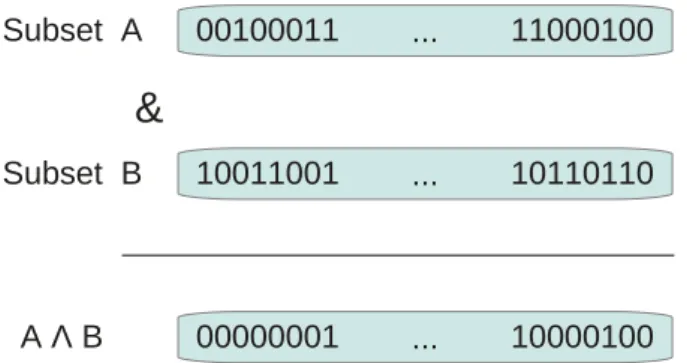
2.6 Parallelization in bioinformatics ... Subset A 00100011 11000100 ... Subset B 10011001 10110110
&
... A Λ B 00000001 10000100Figure 2.5.2: Bit parallel intersection of subsets. Using a logic and between these two bit vectors yields the expected result.
2.5.2 Bit-level parallelism
Bit-level parallelism relies on the same principle as vector instructions except that instead of increasing the size of the registers, we reduce the size of the data items. Several smaller data items can be packed into a single register and computed simul-taneously using traditional word size instruction or even vector instructions.
A typical bit-level parallelism example consists in representing subsets of a larger set of size N using a bit vector the length of the super-set. The nth bit in the bit vector represents the presence or absence of the nth item in the subset. In this case,
every bit of the subset is a data item. The intersection of two such subsets can then be obtained in a reduce number of instructions using a simple logic and operation - see Fig. 2.5.2. The number of instructions required for such an operation thus is
N/RS, where RS is the size of the register. In the same way, a logic or yields the
union of the two subsets. Inclusion of a subset A in a subset B can be tested by an equality test between the result of A ∧ B and subset A.
2.5.3 Instruction-level parallelism
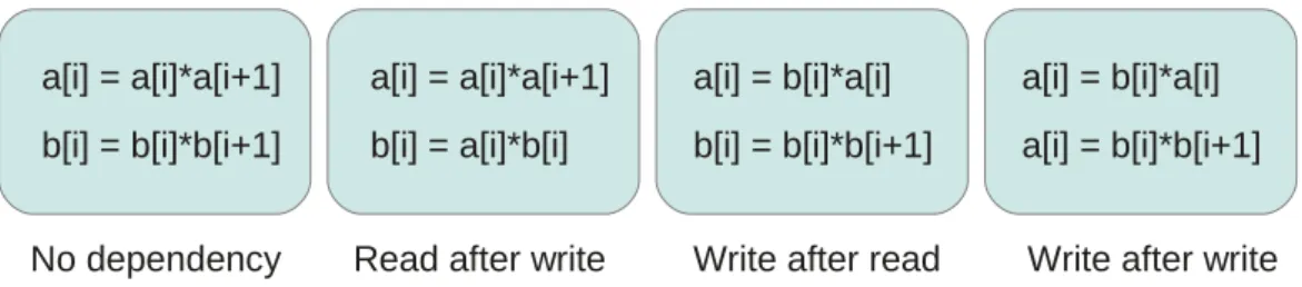
Instruction-level parallelism (ILP) refers to the simultaneous execution by a single processor of independent instructions belonging to a similar code region. Two in-structions are considered independent if one does not read nor write a value that is written by the other - see Fig. 2.5.3. ILP is not directly the responsibility of the programmer and is exploited by the compiler and the hardware but knowing how ILP works may let programmers write code that will allow the compiler to increase the amount of ILP. Several techniques, such as loop unrolling, may favor ILP.
2.6 Parallelization in bioinformatics
Bioinformatics as a field of research encompasses a wide variety of data and computa-tion intensive problems. Recent technologies, such as Next Generacomputa-tions Sequencers (NGS), have greatly increased the amount of data to process for a single analysis,
a[i] = a[i]*a[i+1] b[i] = b[i]*b[i+1] a[i] = a[i]*a[i+1] b[i] = a[i]*b[i] a[i] = b[i]*a[i] b[i] = b[i]*b[i+1] a[i] = b[i]*a[i] a[i] = b[i]*b[i+1]
No dependency Read after write Write after read Write after write
Figure 2.5.3: Examples of possible dependencies between two instructions. thus accentuating the need for efficient implementations in a large array of known problems. The aim of this section is to give a non exhaustive list of problems impor-tant to bioinformaticians that have benefited from one or more forms of parallelism. When available, speedups claimed by the original authors are also reported in this section. However, these speedups should not be compared directly, since reference times were not taken on similar architectures.
2.6.1 Sequence comparison
Sequence comparison is a central topic in bioinformatics. Comparing DNA, RNA or protein sequences allows bioinformaticians to study the functional, structural or evolutionary relationships between two sequences that may come from a single individual, two individuals from a same species or even individuals from different species. The recent exponential increase in the amount of data available has stressed the need for efficient implementations, taking advantage of all the available compu-tational power. In this context, many parallel implementation have been proposed. 2.6.1.1 Sequence alignment
Sequence alignment in bioinformatics is, from a computer science point of view, string alignment over a very succinct alphabet. Therefore, bioinformatics relies heavily on advances made in computer science. Aligning two sequences consists in finding the superpositions of the two sequences that minimize the number of mismatched characters. Gaps may be introduced in either sequence to allow a better superposition of the two sequences. A gap penalty must be applied to minimize the number of gaps.
[Mye99] proposed an elegant bit-parallel algorithm for approximate string match-ing based on dynamic programmmatch-ing. This algorithm was recently adapted to DNA sequence alignment by [KKN12]. In this implementation, the authors did not compare execution times with a previous non bit-parallel implementation, thus no speedup is reported here. They however estimated the comparison time to 28 ns per base pair including file I/O on an Intel Xeon E5540 (2.53 GHz) PC. More re-cently, [Edg04] proposed a bit-parallel improvement of their own software named MUSCLE, a tool for creating multiple protein sequence alignments. In this im-proved implementation, a bit vector is used to represent the presence or absence of
2.6 Parallelization in bioinformatics
k-mers in a given sequence; a k-mer being a subsequence of length k. In this
rep-resentation, the nth bit is set if the nth k-mer is present in the sequence and unset
otherwise. This representation allows MUSCLE to quickly compute set operations such as intersection of two sets - see sec. 2.5.2.
Vector instructions have also been used to speed up sequence alignment programs. [Far07] proposed a very efficient implementation of the Smith-Waterman algorithm that takes advantage of Intel SSE2 intrinsic functions. The performance of their implementation greatly surpassed that of other SSE implementations of the same algorithm, namely [Woz97, RS00].
Sequence alignment has also been extensively parallelized over multicore CPUs. [KT10] proposed a threaded implementation of MAFFT, a program for multiple sequence alignment. Their parallel implementation scales decently up to about 10 CPU threads on a machine with a 16 core CPU. In terms of results, [KT10] obtained a slightly lower accuracy than [Edg04] with much longer runtimes. [LSM10b] also proposed a multicore implementation of a program for multiple sequence alignment called MSAProbs. No information is given about how well their implementation scales with the number of applied threads; they however show that their results obtain better accuracy scores than [Edg04, KT10] but for runtimes even longer than [KT10]. [L+09] also proposed a local alignment tool named Plast that takes
advantage of both SSE instructions and multicore parallelization.
Programs taking advantage of GPUs for sequence alignment started to appear from the beginning of the GPGPU era with [LHJV06] for local sequence alignment and [LSVMW06, WSVMW07] for multiple alignments. All of these programs used graphics libraries to offset computations to the GPU as neither CUDA nor OpenCL existed then. When CUDA was released by NVidia in 2007, new programs emerged benefiting from the enhanced programmability of GPUS. [MV08, LR09] improved previous performances on GPUs for local sequence alignment and [LSM09] for mul-tiple sequence alignment. More recent efforts by [LSM10a, VS11, ZC13] focused on improving with GPUs the performances of BLAST [AGM+90], the reference in local
alignment search.
2.6.1.2 The longest common subsequence problem
Given two strings, the longest common subsequence problem (LCS) consists in find-ing the longest sequence common to both strfind-ings. A subsequence differs from a substring in the sense that some characters from a given substring can be omitted to form a substring. For example, CAT is a subsequence of the string CAGT , where the character G is omitted. The generalization of this problem to an arbitrary num-ber of strings is called the multiple longest common subsequence problem (MLCS). The MLCS problem is known to be NP-hard, whereas the LCS problem can be solved in polynomial time. Both problems are generally tackled using dynamic pro-gramming (DP) techniques; parallel implementations for both problems thus mostly rely on parallel DP techniques.
is used as a similarity measure between the two sequences. As mentioned previously, sequence similarity may indicate an evolutionary relation between two sequences. Such similarity measures can be used in phylogeny for classification purposes or to determine whether two proteins can have similar functions.
However, the LCS problem does not take into account any prior biological knowl-edge for the found longest common subsequence. To address this issue, [Tsa03, TLC+03] formalized the Constrained Longest Common Subsequence problem (CLCS).
The CLCS problem restricts the output of the LCS problem to subsequences con-taining a given subsequence P ; for two input sequences M and N , only common subsequences of M and N containing P are considered. Biological knowledge can be incorporated in this additional constraint.
[Hyy04] proposed a bit-parallel solution to the LCS problem and improved two existing bit-parallel implementations by [AD86, CIPR01]. [Hyy04] compared his implementation to the fastest non-parallel implementation by [KC89] for increasing alphabet sizes. [Hyy04]’s implementation is rather constant with respect to alphabet size and at least twice as fast as that of [KC89], even though the latter is specifically optimized for very large alphabets. [Deo10] also proposed a bit-parallel algorithm but for the recently formulated CLCS problem; the performance of his implemen-tation surpassed all other existing implemenimplemen-tations for this problem and achieved a speedup between 2 and 4 when compared to the fastest known implementation.
Multithreaded implementations exist as well for these problems. In 2011, [WKS11] proposed a new algorithm and it Pthread implementation for the NP-hard MLCS problem. [WKS11] compared their results to that of traditional sequence aligners, namely MUSCLE [Edg04] and ClustalW [THG94]. Since sequence aligners differ from MLCS solvers, [WKS11]’s run-times are much longer but yielded sensibly longer results.
[YXS10] designed a new algorithm for the LCS problem that exhibits more paral-lelism than previous approaches. They proposed two parallel implementations of this new approach: a multicore CPU implementation and a GPU implementation. They compared the run-times achieved by both implementations to that of the sequential implementation from [UI93]. The multicore CPU version performed about 3 times as fast as the sequential version and the GPU version showed a 6 fold speedup over the multicore CPU version.
2.6.2 Structure comparison
Protein three-dimensional structures are more closely related to their functions than protein amino-acid sequences; therefore, structures tend to be more evolutionary preserved than sequences. Finding protein structure similarities thus yields more information about functional similarities than sequence similarities. However, com-paring three-dimensional structures proves more challenging than comcom-paring one-dimensional sequences.
A common way to address the problem of aligning three-dimensional structures is to create an alignment graph or product graph. For two structures S1 and S2 or
2.6 Parallelization in bioinformatics
lengths m and n respectively, an alignment graph of these two structures is an m ∗ n grid shaped graph, where vertex (i, j), located on the ith row and the jth column
corresponds to the matching of the ith element of S
2 with the jth element of S1.
In this alignment graph, an edge between vertices (i1, j1) and (i2, j2) indicates
that matching elements i1 and i2 with elements j1 and j2 in the same alignment
is relevant - see sec. 5.1.1 for a more detailed description of alignment graphs. A common way to add edges top the graph is if, for a given distance function d - often a euclidean distance - d(i1, i2) ≈ d(j1, j2); in other words, if the two distances being
matched are similar in both proteins. In such a graph, a subset of vertices with high edge density denotes a similarity between the two structures.
2.6.2.1 The maximum clique problem
The highest possible edge density in a subset of vertices is achieved when any any two vertices are connected to each other. Such a subset of vertices is called a clique. Finding the largest clique - or one of the largest cliques, as two distinct cliques can be of equal and maximum size - in a given graph is an NP-hard problem referred to as the maximum clique problem. The computational challenge it represents and the large amount of parallelism it induces - testing the presence of all edges in different subsets - seem to make the maximum clique problem a perfect candidate for various parallelization techniques.
A common way to approach the maximum clique problem is through branch and bound techniques. Branch and bound consists in presenting possible solutions in the form of tree. In the case of the maximum clique problem, where a brute force approach would consider every subset of vertices in the input graph, each branch between two levels of the exploration tree denotes the addition of a vertex to the current set of selected vertices. Each node of the tree is therefore a potential solution to the problem. With this representation, a branch and bound approach estimates the potential maximal clique that a given subtree can offer using an approximation. If this potential exceeds the current known best clique, the subtree is explored and pruned otherwise.
Parallelizing the exploration of a branch and bound tree is however challenging and can even lead to a slowdown [LS84]. If multiple threads explore the branch and bound tree in parallel, only communicating to improve the best known solution, the whole tree is explored in a different order than it would in a sequential approach. Some branches that would have been pruned with a sequential traversal of the tree may end up being explored when processed in parallel, thus increasing the total amount of work.
Despite this issue, [TKM07] proposed a multicore solution to the maximum clique problem and achieved substantial speedups when compared to their own sequential implementation. They however compared executions over only 12 randomly gen-erated graphs. We can expect that some other instances may show much poorer results if the lower bound of a clique close to the maximum size is found late in the execution due to a different exploration order of the search tree induced by
parallelism.
A finer type of parallelism is nevertheless achievable without potentially increas-ing the overall workload. Bit-level parallelism is particularly well suited to handle set operations. [SSRLJ11] proposed a bit-parallel implementation for the maximum clique problem and later published an improved version in [SSMRLH13]. This im-proved version obtained better performances on average than the leading program from [TSH+10].
To the best of our knowledge, no GPU implementation exist for the maximum clique problem. The properties of the problem make it difficult to implement ef-ficiently on a GPU; the number of subtasks is unpredictable and these tasks un-balanced. A GPU implementation would greatly suffer from warp divergence and non-coalesced memory accesses. Algorithms that can be used to speedup the branch-and-bound search tree exploration can however be successfully implemented on a GPU. [GZL+11] proposed a GPU implementation of a graph coloring heuristic.
graph coloring heuristics are often used for the maximum clique problem as an up-per bound for the maximum clique that can be found in a branch of the exploration search tree. Graph coloring consists in finding the smallest number of colors required to color a graph so that no two adjacent vertices have the same color. The imple-mentation from [GZL+11] proved that runtimes on the GPU could be equivalent
to that of traditional CPU implementations and yield better approximations of the actual number of required colors.
2.7 Conclusion
Many applications in bioinformatics can benefit from parallelizing techniques. Mod-ern computers nowadays offer a large array of parallel capabilities that range from the fine-grain vector instructions to coarser-grain approaches such as multicore CPU and manycore GPU programming. Each parallelizing technique provides a potential speedups; reaching this theoretical speedup is however almost impossible to achieve depending on the problem to solve.
Each parallelizing technique has its specificities that make it suitable only for some computational problems. Identifying which techniques are susceptible of giv-ing the best speedups for a given problem can be done through a thorough analysis of the problem to solve and a deep comprehension of the hardware. Some problem, known to be inherently sequential, will never benefit from parallelization. Once a po-tentially successful parallelizing technique has been identified, developing a parallel implementation is a tedious and time-consuming process.
Since parallel architectures seem to be becoming the norm in computer architec-ture, new methods and algorithms should be developed early on with parallelism in mind to reduce the cost of a subsequent parallelizing process.
3 GPU accelerated QTL mapping
This chapter discusses a GPU implementation of a QTL mapping tool named QTLMap. QTLMap is developped by the animal genetics division at INRA. The original release dates back to 2008 [GLRM+08]. The tool was later reimplemented
to take advantage of multicore CPUs in 2009. sec. 3.1 first gives an overview of the underlying principles of QTL Mapping. sec. 3.2 then describes the specific methods implemented in QTLMap. sec. 3.3 details the GPU implementation of QTLMap. Finally, sec. 3.4 gives some experimental results. This chapter is mostly based on an article published in the Journal of Computational Biology ([CFE+13]).
3.1 Introduction to QTL mapping
Most of the traits characterizing individuals (their "phenotypes": performance level, susceptibility to disease etc..) are influenced by heredity. Geneticists are interested in detecting, localizing and identifying genes, the polymorphism of which explains a part of observed trait variability. Such genes are often called QTLs (for "Quantitative Trait Locus"), the term locus pointing to a physical position on the genome.
QTL detection procedures consist in a series of statistical hypotheses tests at successive putative locations on the genome. Many experimental designs, sampling protocols and test statistics were proposed and used. QTLMap’s algorithm focuses on regression approaches performed on sets of large families. These approaches were developed for exploiting the linkage disequilibrium - the discrepancy between a random distribution of haplotypes and the observed distribution of haplotypes in the studied population - observed on a per family basis and / or at the population level. Amongst the available software dealing with QTL regression techniques, QTLMap was developed ([EMG+99]).
The general principle of Linkage Analysis (LA) for detecting QTLs within a fam-ily is to correlate for each tested genome position, the performance trait measured in the progenies and the grand parental origins of the piece of chromosome they received from a common parent. These origins are inferred from "genomic marker information" which describe the parental chromosomes (in diploid species, chromo-somes are in pairs and each individual carries two copies, or "alleles", of QTLs, say Q1 and Q2, and markers, say M1/M2, N1/N2) and the way they are transmitted to their progenies (see Fig. 3.1.1). Locations of QTLs are pointed on chromosomal segments, which display high correlations.
Linkage Disequilibrium Analysis (LDA) does not exploit family structure but considers the whole population as a large sample of independent individuals. Due
Figure 3.1.1: Repartition of markers M1/M2 and N1/N2 on alleles Q1 and Q2. to various demographical events along the population histories (selection, breeds mixtures, bottlenecks etc), allelic forms found at two close chromosomal positions are generally not independent. A few measurements of this dependence were proposed in the past ([Lew64, HR68]). This phenomenon is fully proven for markers, which are easy to visualize (e.g. [FCA+00] for the Bovine species) and certainly true between
markers and QTLs.
In LDA, the direct effect of genetic information (to make presentation simple, say the marker genotype effect) on the quantitative trait variability is tested at successive positions. The basic idea is that groups of individuals defined by their genetic class (e.g. their genotype for the marker located at the tested position) will display significant differences in their quantitative performance if a QTL is located close to this position. The signal will be stronger if:
1. the linkage disequilibrium between markers and QTL is higher and 2. the QTL explains a larger part of the variability.
A third category of techniques combines LA and LDA. In Linkage Disequilibrium Linkage Analysis (LDLA), both the family structure and the population history are exploited. The population is described as a set of "founders", supposed un-related, but subject to linkage disequilibrium, and "non-founders" which inherited from the founders, intact or recombinant chromosomes, after one or more genera-tions of transmission. In LDLA, the performance trait measured in the non-founders are correlated, as in the LA, with the founder origins of the transmitted piece of chromosomes, and, as in the LDA, information about the population history is ex-tracted from the degree of similarity between founder pieces of chromosomes. Thus, detecting QTLs is basically a three steps procedure:
1. inferring from the marker information the "phase" of the parents ([EMG+99,
FEDGL10]), i.e. the way the two alleles of each marker are positioned on the chromosomes. The output is the haplotype pairs of each parent, i.e. the list of successive marker alleles carried by each chromosome (e.g. M1N1 and M2N2, or M1N2 and M2N1);