Refinancing risk and its impact on distressed company valuation

(1)

MEMOIRE

P r és ent é en v u e d e l 'o b t ent i o n du M as t er en I ng én i eur d e g es t io n , à f in al it é Ad v anc ed M an ag emen t

Refinancing risk and its impact

on distressed company valuation

Romain Hup

Directeur: Professeur Yassine Boudghene Commissaire: Professeur Catherine Dehon

Année académique 2013-‐ 2014

(2)

(3)

(4)

MEMOIRE

P r és ent é en v u e d e l 'o b t ent i o n du M as t er en I ng én i eur d e g es t io n , à f in al it é Ad v anc ed M an ag emen t

Refinancing risk and its impact

on distressed company valuation

Romain Hup

Directeur: Professeur Yassine Boudghene Commissaire: Professeur Catherine Dehon

Année académique 2013-‐ 2014

(5)

(6)

Abstract

The main objective of this dissertation is to develop a model to assess the impact of refinancing risk on a company value and observe how the latter will react to a refinancing operation. A literature study of the current credit risk models determines that none of these models are designed to take this refinancing risk into account. This dissertation therefore presents a model based on a cash flow approach to value the refinancing exposure of a company. The model concludes that the refinancing exposure represents a hidden debt for a distressed company. This hidden debt locks a part of the firm’s value and has a negative impact on both the equity and debt values of a firm. When a company successfully conducts a refinancing operation that reduces its exposure, the equity and debt values react positively as the hidden debt decreases. These conclusions are verified by the study of five distressed companies.

(7)

Acknowledgements

I would like to express my deep gratitude to Professor Boudghene, my supervisor, for his guidance and useful critiques of this research work. My grateful thanks are also extended to Bernard Lalière, Head of High Yield Fixed Income at Petercam Institutional Asset Management, for his regular feedbacks and valuable support. I also wish to acknowledge the help provided by the whole Institutional Fixed Income department of Petercam in accessing the financial data required to write my dissertation. I also would like to thank my parents for the support and conducive environment they provided me during my whole studies. Finally, my special thanks are extended to my classmates that made this five years at Solvay so exciting, especially Florence, Guillaume, Nicolas and Thibaut.

(8)

Executive Summary

When financing their long-term operations by issuing shorter-term debt, companies are required to refinance their debt on a regular basis and are faced with uncertainty regarding the future underlying interest rate. This situation, known as refinancing risk, may have an important impact on the liquidity of a distressed company and might ultimately force it to default. A distressed company is indeed faced with uncertainty about its future outlooks and will have to pay a premium when refinancing its debt in order to compensate for the increased risk. Intuitively, this premium should therefore negatively influence the value of a firm. On the other hand, the latter is expected to react positively to a refinancing operation.

The goal of this dissertation is to develop a practical model in order to measure the exposure of a firm to the refinancing risk and ultimately confirm or infirm the intuition regarding the impact of this risk on a distressed company value. This dissertation will therefore study the refinancing risk from the perspective of an outside investor. The model presented in this dissertation is based on the Asset Liability Refinancing Gap model developed by Yann Ait Mokhtar for Exane. However, due to the little information publicly available, the model has been adapted and completed by the author.

The methodology used to answer this research question is based on a three-step process. It starts by a literature review of the existing valuation models and observes whether and how they take the refinancing risk into account. It then presents a model specifically designed to value the refinancing risk, the ” Refinancing gap model”, and provides theoretical answers to the research question. Finally, it applies the model to existing companies and observes whether the theoretical conclusions are confirmed by reality. Each step of the process relates to a chapter of the dissertation.

It appears from the literature review that none of the current models takes the refinancing risk into account when modelling the probability of default of a firm and indirectly its value. As a matter of fact classical structural models assume that a company defaults as soon as its firm value falls below a given threshold. Although this threshold depends on the specificities of the model,

(9)

structural models rely only on economic distress to trigger off the default of a firm. By doing so, they fail to take another kind of distress into account, that is to say the financial distress. Financial distress occurs when the company faces difficulties to honour its financial obligations and is therefore considered a cash flows or liquidity issue. Refinancing risk is therefore a subset of this liquidity risk as uncertainty regarding the refinancing terms directly impacts the liquidity of a firm. As a consequence, classical structural models either assume that the company will be able to refinance its total debt under the current terms in the future or that the company will stop existing at the maturity of the outstanding debt. These assumptions are obviously not verified in reality and require the development of a new model to deal with the refinancing risk.

This new model, called the “Refinancing gap model”, is based on a cash flow approach of the refinancing risk. In fact the company has to finance its future activities, yielding a known cash flow, by borrowing at an unknown rate. This situation is similar to a swap position for the company, in which it receives fixed cash flows from operating activities and has to pay an interest rate on its future debt that will only be determined when the debt is rolled over. This swap should be considered an off balance sheet item and is similar to a hidden debt in the case of a distressed company whose expected refinancing terms have worsened. The value of this swap represents the exposure of the firm to the refinancing risk. As this exposure is considered a hidden debt, it directly influences the value of both equity and debt. On one hand, this hidden debt increases the total leverage of the firm, hence the credit risk of the debt. As a consequence, the credit spread on the debt will also increase, which will negatively impact the value of the debt. On the other hand, the hidden debt represents the part of the value of the firm which is locked due to the refinancing exposure and is therefore currently not available for the shareholders, resulting in a lower value of the equity. As part of the value of the firm is therefore locked and not attributed to either the shareholders or the debt holders, the actual value of the firm, equal to the sum of the equity and he debt value, is lower than the one of a similar firm without exposure to the refinancing risk.

A distressed company with an exposure to the refinancing risk has various options to reduce this exposure. These operations (i.e. capital increase, assets disposal, etc) will have a positive impact on the liquidity of the firm, hence reducing the exposure and the value of the hidden debt. In turn

(10)

a reduction in the hidden debt will positively affect the equity and debt value, hence the actual firm value. On one hand, the reduction in the hidden debt decreases the leverage of the firm and consequently its credit risk. On the other hand, the refinancing operation will unlock part of the firm value, which will directly be transferred to the equity.

In theory the refinancing gap model is therefore able to explain how the refinancing exposure affects a firm value and how the latter reacts to refinancing operations. The model was finally applied on existing companies to test whether it predicts accurately the equity and debt value of distressed companies in real terms. It turned out that the refinancing gap model is efficient to predict the stock price of distressed companies and improves the accuracy of classical structural models when forecasting the bond spread.

Indeed the refinancing gap model has successfully predicted the stock prices of the four studied companies presenting a positive refinancing exposure, both before and after the refinancing operations. Furthermore, it outperformed significantly the classical structural models used as a benchmark. Moreover, the model successfully predicts the magnitude of the stock price variation when the firm announces its refinancing operations, which is impossible by means of the classical structural models. It is clear that these models provide forecasts that are usually contrary to the stock market reaction. Considering that the refinancing exposure locks part of the value of the firm to the detriment of the shareholders therefore appears to be a relevant approach. Moreover this is in line with the stock market reaction to such exposure.

On the other hand, the refinancing gap model systematically predicts bond spreads that are higher than those of classical structural models, hence improving the accuracy of these models. Moreover, the biggest improvements appear for companies that face a considerable refinancing exposure. As a consequence, it proofs that the refinancing risk significantly impacts the bond spread of a distressed company and justifies partly the “underprediction” of the classical structural models. However, the Refinancing gap model still fails to accurately predict the real bond spread and only provides a closer estimation. By considering the refinancing risk in addition to the economic distress, the refinancing gap model therefore takes into account a wider range of financial triggers. However, the refinancing gap model does not consider the liquidity issue in its

(11)

broad sense. This limitation might explain the remaining difference between modelled and observed spreads

Following these conclusions about the refinancing gap model as well as its limitations, improvements to this model can be proposed as future research directions. Firstly, a statistically significant quantitative study could be conducted to confirm or infirm the results of this dissertation. Secondly, other proxies for the refinancing premium could be used. Finally, the accuracy of the refinancing gap model could be improved by trying to include the liquidity risk in general or by using more advanced, computing-intensive structural models.

(12)

Introduction

In November 2008 Standard & Poor’s1 announced that 1,6 trillion euros of European debt would mature over the next three years in a context of unfavourable bond market conditions. As a consequence, Standard & Poor’s warned that a growing number of companies might have to struggle to refinance their debt resulting in a refinancing cost which will be on average 200bp higher than before August 2007. When financing their long-term operations by issuing shorter-term debt, companies are indeed required to refinance their debt on a regular basis and are faced with uncertainty regarding the future underlying interest rate. This situation, known as refinancing risk, may have an important impact on the liquidity of a distressed company and might ultimately force it to default. A distressed company is indeed faced with uncertainty about its future outlooks and will have to pay a premium when refinancing its debt in order to compensate for the increased risk. Intuitively, this premium should therefore negatively influence the value of a firm. On the other hand, the latter is expected to react positively to a refinancing operation.

The goal of this dissertation is threefold: to develop a practical model to measure the exposure of a firm to the refinancing risk and ultimately confirm or infirm the intuition regarding the impact of this refinancing risk on a distressed company valuation and finally observe how the latter reacts to a refinancing operation. In the framework of the dissertation, a distressed company is defined as a company whose outstanding debt is considered speculative by rating agencies. Moreover, the company value will be studied from the point of view of the equity (stock price) and debt (bond spread) values. Finally, a refinancing operation will be defined as an operation that reduces the refinancing exposure of the company. This dissertation will therefore study the refinancing risk from the perspective of an outside investor. The approach of this dissertation will be exhaustive and detailed in order to allow any financial investor to apply the model in practice, whatever his level of knowledge in credit risk modelling.

1_{STANDARD & POOR’S, “}_{Credit Trends: Gaping Refunding Pipeline In Europe Intensifies Financial Challenges}_“_,

(16)

The methodology used to answer this research question is based on a three-step process. It starts by a literature review of the existing valuation models and observes whether and how they take the refinancing risk into account. It then presents a model specifically designed to value the refinancing risk, the ” Refinancing gap model”, and provides theoretical answers to the research question. Finally, it applies the model to existing companies and observes whether the theoretical conclusions are confirmed by reality. Each step of the process relates to a chapter of the dissertation.

The first chapter of the dissertation will start with an introduction of the credit risk and its measurement. Then it will highlight the different reasons that may trigger off the default of a company and define one of them, more specifically the refinancing risk. It then presents the different ways to forecast the credit risk and deep dives into one of them, the structural model. In this section, the intuition and limitation of the most famous structural models (Merton and CreditGrades amongst others) will be introduced. Finally, the last section will study whether structural models take the refinancing risk into account or not.

The second chapter starts by introducing the intuition of the Refinancing gap model and presents step by step how to apply it, based on a practical framework. It then explains how this refinancing gap impacts a firm’s value and how to adapt the structural models to take the refinancing risk into account. Finally, it highlights the different actions that a distressed company can take to solve its liquidity issues and the impact these have on the company value, in the light of the refinancing gap.

The last chapter represents the practical implementation of the Refinancing gap model presented in chapter 2. It will study five companies that all faced an important exposure to the refinancing risk and decided to use one or several of the refinancing operations introduced in chapter 2 to reduce this risk. For each company, it will present the background of the firm as well as the reasons that led to the refinancing exposure. It will also use the refinancing gap model to compute both the equity and debt values of the firm and compare them with classical structural model estimations. It will then explain the refinancing operation and compare the predicted outcome (by

(17)

the refinancing gap model and classical structural model) with the reality. Finally, it extends the model to a company facing a negative exposure to refinancing risk

Finally, the conclusion presents the limitations of the Refinancing gap model and proposes four research directions to complement this dissertation and improve the Refinancing gap model.

The refinancing gap model presented in this dissertation is based on a model initially developed by Yann Ait Mokhtar for Exane and called the “Asset Liability Refinancing gap”. However, as this model has been developed internally by a financial company, little information is publicly available. This dissertation is therefore based on the author’s interpretation of the information available and has been completed by his own research. Moreover, due to the amount of time required to become familiar with a company history and apply the model in practice, this dissertation will focus on a relatively limited panel of companies. Therefore this dissertation does not aim at providing a statistically exhaustive confirmation of the refinancing gap model through a quantitative study. Instead, it aims at showing the intuition of the refinancing gap models through relevant cases.

(18)

Chapter 1 Refinancing risk and literature review

A company with a maturing debt is facing uncertainty about the conditions under which it will be able to refinance it. This issue, known as refinancing risk, can affect significantly the liquidity of a company and force it to default. Refinancing risk is therefore a subset of the credit risk. The goal of this chapter is to present the main models forecasting credit risk, observe how they potentially take into account the refinancing risk and highlight their limitations.

The first section of this chapter will introduce the credit risk and its measurement. Then it will highlight the different reasons that can trigger off the default of a company and define one of them, i.e. the refinancing risk. The second section will present the different ways to forecast the credit risk while the third one deep dives into one of them, the structural model. In this section, the intuition and limitation of the most famous structural models will be introduced. Finally, the last section will study whether structural models take the refinancing risk into account or not.

Section 1: introduction to credit and refinancing risk

When entering into a financial transaction, an investor is facing several risks, the more important ones being the market risk and the credit risk. The market risk2 is “the risk of a change in value of a financial asset due to a change in the market conditions (interest and exchange rates amongst others)”. The market risk is therefore not linked directly with a single company or a financial product.

On the other hand, the credit risk3 is “the risk that an issuer might default or fail to fulfil entirely his obligation due to a change in its credit quality”. The credit risk therefore depends on the

2 _{DARRELL, Duffie and SCHAEFER ,Stephen, Credit Risk: Pricing, Measurement, and Management, Princeton,}

Princeton University Press, 2003, p.3.

(19)

issuer and can lead to large losses for the lender. As a consequence, the latter will require to be rewarded for his exposure to this risk. This reward will take the form of a premium on the risk-free interest rate used when there is no credit risk. The premium therefore represents the compensation for the risk of default and is computed accordingly.

1.1 Credit risk measurement

In order to assess the credit risk of a counterparty, financial regulators have developed several frameworks. Amongst them, Basel and its subsequent updates are the most famous ones. The bank of the International Settlements laid down the Basel rules in 1988 to allow all lenders to measure the possible credit risk in a coherent and similar way and to make sure they have put aside enough capital to face potential credit losses. This approach has been developed for financial institutions but can be used by any investor.

Basel defines4 credit risk as:

« The risk of loss from a borrower/counterparty’s failure to repay the amount owed (principal or interest) to the bank on a timely manner based on a previously agreed payment schedule ». A more comprehensive definition also includes value risk5:

« The risk of loss of value from a borrower migrating to a lower credit rating (opportunity cost of not pricing the loan correctly for its new level of risk) without having defaulted ».

In order to model the credit risk, Basel used the following formula6: EL = PD * EAD * LGD

4_{STEPHANOU, Constantinos, and Juan Carlos Mendoza. "Credit risk measurement under Basel II: an overview and}

implementation issues for developing countries." World Bank Policy Research Working Paper 3556 (2005), p.6.

5_Ibid. 6_ibid.

(20)

Where:

• EL is the expected loss over a period of time of a financial product or a portfolio • PD is the probability of default over a period of time

• EAD, or exposure at default, is the amount due to the counterparty at the moment of default. It is therefore a measure of the extend to which an investor is exposed to the counterparty in case of a default event

• LGD, or loss given default, is the fraction of exposure that will be lost in the event of default

While the exposure at default is constantly known for a company, the probability of default and the loss given default are uncertain and must therefore be predicted by models. In order to accurately work, these models must take into account all the reasons that may force a company to default. These reasons are presented in the next section.

1.2 Study of default triggers

According to Davydenko7, several reasons can lead to the default of a firm. He divides them into two categories: financial and economic distress. Financial distress occurs when the company faces difficulties to honour its financial obligations. Although the business might seem fundamentally sound, a temporary decline in cash flows may result in the inability of the firm to make the scheduled debt payments. On the other hand, economic distress arises when the prospects of the firm are deteriorating and the value of the business is decreasing. Financial distress can therefore be seen as a cash flow issue, while economic distress is linked to the value of a company.

Davydenko observes that at default, most firms are both economically and financially insolvent. On average, the market value of assets at default is equal to only 60% of the face value of debt. Moreover, liquidity ratios are below the industry median in 80% of the defaulting firms. He concludes that8_{“persistent economic distress seems to drive financial distress”. Indeed, firms in}

7_{DAVYDENKO, Sergei A. "When do firms default? A study of the default boundary." A Study of the Default Boundary} (November 2012). EFA Moscow Meetings Paper. 2012, p.2.

(21)

economic distress are losing money and therefore need to sell their liquid assets to pay the money back to their creditors and suppliers until they reach financial distress. However, this conclusion should not be seen as a generality. Low-value firms are distinct from low-liquidity firms in a substantial amount of observed default events. Around 13% of firms default with low asset value despite their liquid assets in excess of current liabilities. Furthermore, at least 10% of firms default, although their asset value is higher than the face value of debt. These firms are therefore economically solvent, but have major liquidity problems triggering off the default event. Finally, many distressed low-value and low-liquidity firms are able to postpone default over several years. Indeed, a majority of economically insolvent companies succeed in delaying the default for at least a year. Davydenko concludes that neither economic nor financial distress taken alone can fully explain the default of a company.

Moreover, as different firms default at very different asset values and as there are as many firms defaulting when their assets are low as the firms that do not, it is hard to define a boundary separating defaulting from surviving companies. Davydenko and Leland9 both determine the threshold value “of assets that equalizes the number of defaults above the boundary with the number of no defaulting firms below it » as being equal to 68% of the face value of debt. Leland found that structural models calibrated with this threshold generate on average long-term default probabilities that are in line with the observed data. Although appealing at first glance, the Davydenko study yields totally different results when companies are analysed on an individual basis: one-third of defaults occurs at values above this boundary and could not be predicted by structural models. Moreover, an equal number of companies below it do not default for a least one year, although the default had been predicted by structural models.

As explained by Davydenko, a transitory liquidity problem can trigger off default, if the firm is prevented from raising new financing against its assets. If the required amount of cash cannot be raised, the temporary liquidity issue will force the firm to default, despite its sound economic fundamentals. In his study, Davydenko10 found that liquidity shortages lead to default only when

9_{LELAND, Hayne E. "Predictions of default probabilities in structural models of debt." The credit market handbook:} Advanced modeling issues (H. Gifford Fong, Editor) (2006), p.42.

10_{DAVYDENKO, Sergei A. "When do firms default? A study of the default boundary." A Study of the Default}

Boundary (November 2012). EFA Moscow Meetings Paper. 2012, p.8.

(22)

external financing is hard to obtain due to restrictive covenants or a depressed state of the market In the absence of such restriction, firms will raise new cash to overcome liquidity shortages as long as the business remains valuable. Therefore, if external financing is costless, the firm does not default, except in case of economic distress. Between those two extreme situations, the firm might be able to raise new financing to face its liquidity issue and refinance its debt albeit under unfavourable terms. If the company is in a distressed setting, it might indeed have to pay a premium on its debt. This premium will worsen even more the financial distress of the company and eventually trigger default sooner than expected.

This problem, known as refinancing risk, is presented in the next section and is a subset of the credit risk.

1.3 Refinancing risk

Refinancing risk relates11_{to the uncertainty regarding the terms and conditions when a company} has to refinance its debt. When the firm issues new bonds to replace the maturing ones, the market price of the new bonds can be higher or lower than the required principal payments of the maturing bonds. Depending on the market conditions and the fundamentals of the firm, a profit or a loss can therefore occur, when the debt is refinanced. In the extreme case, the firm might be unable to refinance its debt and has to default. The notion of refinancing can be extended to any need of cash to solve a liquidity issue. This is the uncertainty in general about the cost of issuing new debt.

Refinancing a debt is also known as rolling it over; hence refinancing risk is also called rollover risk.

(23)

Section 2: Credit risk modelling

Over the last decades, researchers and practitioners have developed a large number of models to assess the probability of default of a company. The relevant literature divides these models into two categories, the ones using accounting information and the others using the market price of financial assets. These different approaches are presented in the subsection underneath. Moreover, the limitations of each approach regarding the refinancing risk assessment are highlighted.

2.1 Accounting based models

2.1.1 Econometrics models

These models12 use data from the financial statements to forecast a company’s bankruptcy risk. This was originally done through a regression analysis with discriminating factors, but has recently evolved to Probit and Logit models to define a function S of the form:

S(xi) = β1x1 + β2x2 +… + βnxn

The vector 𝑋 contains the relevant risk factors which depend on the company profile (industry, privately vs. publicly owned, etc). The table 1 presents an overview of typically used factors in these models.

12_{STEPHANOU, Constantinos, and Juan Carlos Mendoza. Credit risk measurement under Basel II: an overview and}

(24)

Table 1: Overview of typically used factors in econometrics models13

Information category Parameters

Company type

Industry group Geography Age of company

Total sales / assets / equity

Financial Ratios Equity/assets Debt/equity Sales/assets Profitability Historical profitability Profitability growth rate Profit/ assets

Market data Volatility of stock price

The outcome of econometric models may either be a ranking of the probability of default of several companies or an assessment of the risk of default of a given company.

2.1.1.1 Altman Z-Score

The most famous of these models is the Score developed by Edward Altman in 1968. The Z-score is a combination of five weighted business ratios used to estimate the likelihood of financial distress, as described in the following formula:

(25)

Z = 1.2*T1 + 1.4*T2 + 3.3*T3 + 0.6*T4 + 1.0*T5 where14_:

T1 = Working Capital / Total Assets. It’s a measure of the net liquid assets of the firm relative to the total capitalization. Shrinking liquidity is a warning sign of financial trouble

T2 = Retained earnings / Total assets. This is a measure of the cumulative profitability of the company over time

T3 = Earnings Before Interest and Taxes / Total Assets. This ratio is a measure of the true productivity of the firm’s assets, independent of any tax or leverage factor

T4 = Market Value of Equity / Book Value of Total Liabilities. It’s a measure of how much the firm’s assets can decline in value before the liabilities exceed the assets and the firm becomes insolvent.

T5 = Sales/ Total Assets. The ratio is a measure of how effectively the firm uses its assets to generate sales.

Companies15 with a Z-Score above 2,99 are considered being in the safe zone and thereby not likely to fall into bankruptcy. Those with a Z Score between 1,8 and 2,99 are located in the grey area, meaning that their future is uncertain and that there is a chance the company goes bankrupt within the next two years of operations. Finally, companies with a Z-Score below 1, 80 are in the distress zone indicating a high probability of bankruptcy over the short term.

The initial formula has been defined by studying publicly traded manufacturing companies. Altman and other researchers have developed new models to deal with private and non-manufacturing companies. Moreover, they have continuously updated the parameters of the model taking into account recent market trends.

In its initial paper, Altman16 claims that the model is 72% accurate in predicting bankruptcy over a two-year window. Moreover, in 200017, Altman ran subsequent tests and found out that the

14_{ALTMAN, Edward I. "Predicting financial distress of companies: revisiting the Z-score and ZETA models." Stern} School of Business, New York University (2000), p.10.

15_{ALTMAN, Edward I. "Financial ratios, discriminant analysis and the prediction of corporate bankruptcy." The journal} of finance 23.4 (1968), p.602.

16_ibid.

(26)

updated versions of the model were accurate in 80 to 90% of the cases to predict bankruptcy over a one-year window.

2.1.1.2 Econometrics models and refinancing risk

Although none of the famous econometrics models are taking the refinancing risk into account, these models could be designed to include it. One can indeed add a factor that serves as a proxy for the refinancing risk such as the credit premium (expected future refinancing rate minus current one). However, the aim of these econometrics models is not predicting when a firm will actually go bankrupt, but rather measuring how closely a firm looks like other companies that have previously filed a petition in bankruptcy. These models therefore fail to predict the probability of default of a company and can not be used to predict the impact of the refinancing risk on the value of a firm.

2.1.2 Credit rating models

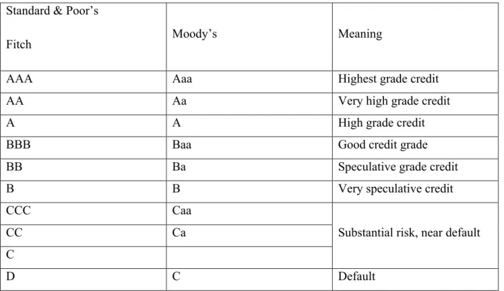
Credit rating models are models created by rating agencies to assess the creditworthiness of a company, hence its credit risk level. A rating can either be allocated to a company in general or to a specific bond in particular and is an indication of the future credit risk of this company or bond. The credit rating represents the opinion of a particular rating agency about the ability and willingness of an issuer to meet his financial obligations. Therefore, different rating agencies may grant a different rating to the same company. There are three major rating agencies: Fitch, Standard & Poor’s and Moodie’s. Each of them uses a specific grading hierarchy for both short and long-term obligations. The table 218 shows the correspondence between the three companies and their meaning.

School of Business, New York University (2000), p.18.

18_{BANK FOR INTERNATIONAL SETTLEMENT. “Long-term Rating Scales Comparison.“ www.bis.org. n.d. 24 Mai}

(27)

Table 2: Comparison of long -‐term credit ratings between agencies and their meaning

Standard & Poor’s

Fitch Moody’s Meaning

AAA Aaa Highest grade credit

AA Aa Very high grade credit

A A High grade credit

BBB Baa Good credit grade

BB Ba Speculative grade credit

B B Very speculative credit

CCC Caa

Substantial risk, near default

CC Ca

C

D C Default

Companies with a rating higher or equal to BBB are called “investment grade” companies, while those with a lower rating are named “Junk, high yield, speculative or non-investment grade”.

2.1.2.1 Moody’s methodology

Each rating agency uses its own methodology to determine the ranking of a given company. The one developed by Moody’s is based19_{on a multi-factor analysis. Moody’s analysts determine a} set of key-factors that fall into two categories: the global, where factors are common to all companies in any industry and the industry-oriented which are selected to capture the specificity of a given industry. These factors can be either qualitative or quantitative and are constantly updated. Quality and experience of management as well as assessment of corporate governance are some of the global factors. Examples of industry-oriented ones include size and efficiency of a fleet for the shipping industry. Each factor is subdivided into several sub-factors to which a particular weight is then allocated. Each sub-factor is calculated for the studied company and is

(28)

allocated a rating factor, based on a mapping grid specific to each sub-factor. Finally, Moody’s analysts use a last grid to compute the final rating based on each sub-factor weight. Once the rating has been computed by the analysts, the outcome is presented to the rating committee that might decide to adjust the rating to take into account company-specific elements that are not included in the multi-factor analysis, such as regulatory and litigation risk.

Based on historical data, each rating agency computes the probability that a company with a given rating defaults within a certain timeframe. Credit ratings can therefore be used to compute the probability of default. The figure 1 provides the cumulative probability of default for timeframes going from one year to twenty for each Moody’s rating.

Figure 1: Moody's cumulative default rates between 1970 and 200820

The observed probability of default largely differs across ratings, a lower rating leading to a higher probability of default. As mentioned by Hull21, the probability of default of the investment grade category tends to be a direct, growing function of the horizon. High rated companies are indeed considered to be financially healthy in their first year but as time passes, the probability of encountering financial distress increases. On the other hand, while the probability of default of

20 _{MOODY’S INVESTORS SERVICE. " Corporate Default and Recovery Rates, 1920-2010." (2011), p.24.} 21 _{HULL, John. Options, futures and other derivatives. Pearson education, 2012. 2}nd_{ed. p.522.}

0 10 20 30 40 50 60 70 80 1 2 3 4 5 6 7 8 9 10 11 12 13 14 15 16 17 18 19 20

Cumulative probability of default

(in % ) Years Aaa AaA A Baa Ba B Caa-‐C

(29)

initially lower rated companies also increases with the horizon, the marginal probability is decreasing. Hull explains22 this observation by the fact that the first years are critical for initially unhealthy companies. Once they have survived this trouble period, they will usually recover so that the marginal probability decreases afterwards. Moreover, the graph shows that probability of default is always positive whatever the horizon, even short term, except for the highest rated companies.

2.1.2.2 Credit rating models and refinancing risk

Credit rating models are effectively taking the refinancing risk into account. Rating agencies indeed look at the refinancing exposure either directly in their model as a global factor or indirectly by adjusting the rating during the rating committee to reflect the risk. However, although company rating is an appealing source of information regarding credit risk, one must be cautious when using it as a prediction of default probability. Such probability is indeed computed, using a historical set of data comprising companies of similar risk-profile but with a different history. Moreover, credit ratings are not frequently updated and therefore do not offer the most up-to-date information. For all these reasons, credit rating models are not efficient to predict the impact of refinancing risk on the value of a firm.

2.2 Market based models

As previously mentioned, the market-based models use the market price of financial products to extract the probability of default of a company. There are two different categories of market-based models, namely the reduced form and the structural one. The differences between both categories lie in the assumptions regarding information as well as the default trigger.

Reduced form models23 are developed to take into account the sudden nature of a default. Hence, they consider default an exogenous event driven by a stochastic process. Therefore, they assume24 that a firm default is an unexpected event, whose likelihood is driven by a default- default- default- default- default- default- default- default- default- default- default- default- default- default- default- default- default- default- default- default- default- default- default- default- default- default- default- default- default- default- default- default- default- default- default- default- default- default- default- default- default- default- default- default- default- default- default- default- default- default- default- default- default- default- default- default-

22_ibid.

23 _{WANG, Yu. Structural Credit Risk Modeling: Merton and Beyond. Risk Management 16 (2009). p.30.}

(30)

intensity process, such as the Poisson Jump process.25 Such default intensity process is extracted26 from the market price of defaultable financial instruments such as credit default swaps and bonds. As a consequence, the market is the only source of information that reduced form models use to model credit risk.

Structural models were initiated by Merton in 1974 and aim to provide a relationship between default risk and capital structure. They assume27 that a company will default when it is unable or unwilling to meet its financial obligation. The default is thus an endogenous event and will occur when the assets value of the company will fall below a given threshold. The assets value is modelled as a stochastic process and the threshold varies according to the structural model considered.

Structural models therefore assume28 the perfect knowledge of a precise set of information, akin to the ones held by companies internally. This perfect information assumption therefore implies that the default is predictable. On the other hand, reduced form models only rely on observable data from the financial markets. Therefore, the restricted information makes the default unpredictable. Based on this information, Jarrow and Protter29 claim that the key distinction between both categories is not the characteristic of the default time (predictable versus unpredictable) but rather the range of information available. They also show that by reducing or narrowing the information set available, a structural model can be transformed into a reduced form one.

The main disadvantage30 of the structural models is their difficulty of implementation. They are indeed analytically complex and computationally intensive. Reduced form models, on the other hand, are easy to implement and calibrate, but lag behind regarding their prediction power. In the

25 _{In probability theory, a Poisson process is a stochastic process that counts the number of events and the time}

points at which these events occur in a given time interval

26_{ELIZALDE, Abel. Credit risk models III: reconciliation reduced-structural models. 2006. p.1.} 27 _{ELIZALDE, Abel. Credit risk models II: Credit risk models II: Structural models. 2005. p.1.}

28 _{JARROW, Robert A., and PHILIP Protter. "Structural vs reduced form models: A new information based}

perspective." Journal of Investment Management 2.2 (2004). p.2.

29_ibid

(31)

first attempt to compare both categories, Arora and al31 show that structural models constantly outperformed reduced form ones in both default and spread forecasting.

Moreover, as mentioned by Elizalde32, reduced form models, by relying on exogenous events, “lack the link between credit risk and the information regarding the firms’ financial situation incorporated in their assets and liabilities”. They are therefore less able to provide interpretation to default event.

For these reasons, structural models are widely used in counterparty credit risk analysis and capital structure monitoring, while reduced-form ones are used on credit security trading floors.

2.2.1. Market based models and refinancing risk

Reduced form models indirectly take into account the refinancing risk when modelling the probability of default. The default intensity process of these models is indeed extracted from the market price of defaultable financial instruments. If these financial instruments are correctly priced by the markets, their spreads should therefore reflect the refinancing risk of the underlying company. However, as it is impossible to extract from the market price the part of the spread due to this refinancing exposure, reduced form models do not allow to study the sole effect of the risk on the firm value. Moreover, as it is impossible to accurately predict the future price of these defaultable financial instruments, reduced form models are not useful to study the impact of future refinancing operations.

The link between structural models and refinancing risk will be presented in section 4, following the presentation of the more famous structural models in section 3.

31_{ARORA, Navneet, JEFFREY R. Bohn, and FANLIN Zhu. "Reduced form vs. structural models of credit risk: A case}

study of three models." Journal of Investment Management 3.4 (2005). p.19-20.

(32)

Section 3: Structural models

In this section, the main structural models and their limitation are introduced. Emphasis will be placed on the rationale behind each model. The goal of this section is indeed to provide intuition about how they model the probability of default and what are the factors triggering it.

3.1 Merton model

The first structural model was presented by Merton33 in 1974 in a paper that initiated the use of statistics and mathematics in credit risk modelling. In his paper, Merton develops a framework to link the asset value of a firm to its credit risk. The assumptions and formulas of the Merton model are described in appendix 1.1

3.1.1 Model

Merton built his model by considering the easiest financial structure possible for a firm34: At time t, a given company has assets At, financed by equity Et and coupon debt Dt. This zero-coupon debt has a face value K and a maturity T > t. Thanks to the balance sheet relationship, the following equality obtains:

At = Et + Dt

The pay-off at maturity T of the debt will depend on the asset value. When the value of the firm’s assets at maturity exceeds K, the bondholders receive the full notional amount and the shareholders receive the residual assets value Vt – K.

On the other hand, when the asset value at maturity is lower than K, the firm cannot face its financial obligation and defaults. The company is therefore liquidated and the bondholders receive the firm value Vt , while the shareholders receive nothing. As the shareholders never have to compensate for the bondholder’s loss, the equity value Et cannot be negative.

33_{MERTON, Robert C. "On the pricing of corporate debt: The risk structure of interest rates." The Journal of Finance}

29.2 (1974). p.450.

(33)

Figure 2: Schematic representation of the Merton model35

The figure 2 illustrates the dynamics of the Merton Model. Over time, the total debt is constant and equal to K while the asset value fluctuates. Hence, the total equity value also fluctuates over time and depends on the asset value. As stated before, the firm will only default, if the firm value (equals to the total asset value) at maturity falls below the facial amount of the debt, Vt < K. The facial amount of debt is therefore the default barrier in the Merton Model. One can model the asset value distribution at maturity by simulating various paths for the asset value process, following the stochastic diffusion process presented here above. In the Merton model, the distribution of default is assumed to follow a normal distribution. The shaded area of this distribution is the probability of default.

Based on these observations, the equity value of the company at time T can be written as 36 ET = max (AT-K ;0).

35_{DARRELL Duffie and Stephen Schaefer, Credit Risk: Pricing, Measurement, and Management, Princeton,}

Princeton University Press, 2003, p.54.

36_{SUNDARESAN, Suresh. "A Review of Merton’s Model of the Firm’s Capital Structure with Its Wide Applications."} Annu. Rev. Financ. Econ. 5.1 (2013). p.3.

(34)

This is exactly the payoff of a European call option written on underlying asset AT with strike price K maturing at T. Similarly, the debt value of the company at time T can be written as37 DT = max (A ; K)

This payoff can be replicated with the following portfolio DT = K – max (K-A; 0)

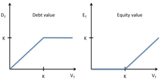
In other words, the payoff of the debt at time T is equivalent to holding the face value of the debt and selling a European put option on the underlying asset AT with strike price K maturing at T. The figure 3 illustrates the payoff of both debt and equity, depending on the asset value

Figure 3: Equity and debt value as a function of the assets value

(35)

The probability of default in the Merton model is therefore given by the probability that the asset’s value at maturity is lower than the facial value of the debt. In other words, the firm will default when the shareholder’s call option on the asset underlying matures out-of-money.

3.1.2 Shortcomings

Although appealing on paper, the Merton model suffers, in practice, from a lack of precision in its predicting power. Van Beem38 studied a panel of Dutch companies and compared the spread predicted with the Merton model with the market data. He observed that modelled spreads are zero for short maturities, as solvent companies are not supposed to default on the short term. However, market data yields a positive credit spread as well as a positive probability of default. He explained this discrepancy by the Merton assumptions regarding the firm’s asset value process. As the process follows a slow evolution, the default event can never happen unexpectedly and the barrier will not be reached within a short period of time.

Moreover, in the long run, credit spread decreases in the Merton model, but is increasing in the market. This is, one more time, due to the assumptions of this model. According to Merton, firms cannot issue additional debt before maturity. As the asset value process includes a positive drift39, the distance between the asset value and the constant facial value of the debt increases and the firm is less likely to default.

Beside these two observations, Sundaresan40_{and Wang}41_{highlight three more shortcomings of} the Merton model.

Firstly, the debt structure of a firm is nearly always more complicated than a simple zero-coupon bond. Debt issued by companies often involves intermediary coupons and covenants42.

Secondly, a firm can only default at debt maturity. Therefore, a firm’s asset value can drop below

38_{VAN BEEM, J. " Credit risk modeling and CDS valuation :An analysis of structural models." University of Twente}

(2010). p.22.

39_ibid.

40 _{SUNDARESAN, Suresh. "A Review of Merton’s Model of the Firm’s Capital Structure with Its Wide Applications."}

Annu. Rev. Financ. Econ. 5.1 (2013). p.5.

41 _{WANG, Yu. "Structural Credit Risk Modeling: Merton and Beyond." Risk Management 16 (2009). p.32.}

42_{A covenant is a promise in an indenture, or any other formal debt agreement, that certain activities will or will not be}

(36)

the facial value of the debt at time t (t < T) and yet recover before maturity. In reality, the firm would have defaulted at t but not according to the Merton model. The Merton model is therefore non-path dependant.

Thirdly, the term structure of interest rate observed in reality is not flat, but varies in time, while the Merton model assumes a constant risk-free rate known with certainty in advance.

3.2 Extensions

3.2.1 Debt structure

As explained before, one of the shortcomings of the Merton model is that the entire debt of a firm is considered a single zero-coupon bond. This simplified situation is totally unrealistic and firms usually issue coupon-bearing debt and attach covenants to the debt issues.

Moreover, the usual valuation technique used to price a coupon-bearing bond, which consists in considering such a coupon-bearing bond as a portfolio of zero-coupons, does not apply to the Merton model. Indeed, if the firm defaults43 on a coupon payment, then it will automatically default on all the subsequent payments. The default on one payment is therefore not independent of the other payment.

A solution to this problem was brought by Geske44. After deriving a formula to price a compound option45_{, he observed that the equity of a company with coupon-bearing debt outstanding, could} be considered such an option. Indeed, at every coupon payment date, the stockholders have the option of buying the next option and keeping the control of the firm by paying the coupon. When they are unable or unwilling to make the payment, they will default on the debt and the bondholders will take over the firm and receive the value of the firm. Similarly, at maturity of the coupon debt, the stockholders have the option to repurchase the claims on the firm from the bondholders by paying off the principal.

43_{MERTON, Robert C. "On the pricing of corporate debt: The risk structure of interest rates." The Journal of Finance}

29.2 (1974). p.460.

44_{GESKE, Robert. The valuation of corporate liabilities as compound options. Journal of Financial and Quantitative} Analysis, 1977, vol. 12, no 04, p. 541-552.

(37)

Although Geske allows considering more complex debt structures than Merton, his structural model still assumes that the default is expected, as the firm can only default at the coupon or principal payment dates.

3.2.2 First-passage model

While the Merton model assumes that a firm only defaults when its value at maturity is below the face value of the debt, in reality a firm can default at any time and for different reasons. The first-passage models have been created to solve the problem of this limitation, as the firm will default when its asset value drops below a given default barrier for the first time. These models46 are therefore path dependant and equity is now modelled as a down-and-out option47. When the asset value of the company reaches the default barrier, the equity will indeed be worth nothing and the company will be liquidated. Such default barrier can be seen as a covenant on the debt and therefore, the value of the debt will be higher than predicted by the Merton model. Similarly, as default may happen at any time, the probability of pay-off to the shareholders is lower and therefore, equity will be worth less than according to the Merton model.

The literature offers a wide range of first-passage models that differentiate themselves by their default barrier specification. They can be classified into two categories: exogenous models that are defined outside the model and endogenous models, where the barrier is defined inside the model.

3.2.2.1 Exogenous barrier

The initial first-passage model, created by Black and Cox48 in 1976 included an exogenous barrier. In such a model, the default barrier is defined outside the model and does not depend on the shareholders. Black and Cox modelled an exponential safety covenant, which allows the debt holders to take control of the firm, when this covenant is breached, in other word when the value of the company is lower than the covenant threshold. The company defaults on its outstanding

46_{BLACK, Fischer and COX, John C. Valuing corporate securities: Some effects of bond indenture provisions. The} Journal of Finance, 1976, vol. 31, no 2, p. 351-367.

47_{A down and out option is an option that ceases to exist when the price of the underlying security hits a specific}

barrier price level

48 _{BLACK, Fischer et COX, John C. Valuing corporate securities: Some effects of bond indenture provisions. The}