T
H
È
S
E
En vue de l'obtention duD
O
C
T
O
R
A
T
D
E
L
’
U
N
I
V
E
R
S
I
T
É
D
E
T
O
U
L
O
U
S
E
Délivré par l'Université Toulouse III - Paul SabatierDiscipline ou spécialité : Écologie et Évolution
JURY
Philipp Heeb (rapporteur)
Nick Royle (examinateur)
Stuart Sharp (examinateur)
Ecole doctorale : SEVAB
Unité de recherche : UMR 5321 - Station d'Écologie Théorique et Expérimentale Directeur(s) de Thèse : Andrew Russell / Alexis Chaine
Rapporteurs : Philipp Heeb
Présentée et soutenue par AISHA COLLEEN BRÜNDL
Le 22 Mars 2018
Titre :
Investissement parental le long d'un gradient altitudinal chez la mésange bleue (Cyanistes caeruleus)
1
Investissement parental le long d'un
gradient altitudinal chez la mésange bleue
3
“When the student is ready the teacher will appear.” (Buddhist proverb)
First and foremost, I would like to thank my supervisors Andy and Alexis for showing me the ways of a scientist and enabling this unique experience of a between-country PhD at two very different, stimulating academic institutes. I am immensely grateful to both of you for believing in my abilities with your relentless support and patient encouragement throughout my PhD. How would I have survived without you teaching me everything; from the practicalities of field work (including changing flat tires on muddy Sunday afternoons) to statistics, writing and presentation skills, and generally keeping my brain from being a coach potato? At times you (and perhaps Andy’s time management) pushed me to my limits, but I would have never learnt as much without these challenges. Many thanks also to Camille for your pastoral care and encouragement.
I am much indebted to NERC, the Midi-Pyrénées region and the Station d'Ecologie Théorique et Expérimentale of the CNRS (UMR5321), in particular to its director Dr Jean Clobert, in ensuring the funds for this PhD. I owe my gratitude to the Universities of Exeter and Toulouse (Paul Sabatier III) and all the people involved in drawing up this first ‘Cotutelle’ agreement between the two universities leading to a joint PhD award. I thank Dalila Booth for translating this agreement. I believe these programmes are imperative in broadening the academic horizon of young scientists, particularly in the current political climate, and I hope to see more of them in the future.
the students and volunteers that participated in the collection of field and lab data and the development of the project over the past few years. The same goes to all the blue tits involuntarily involved in this study. I’m grateful to each and every one of them.
I would like to thank my amazing friends, house mates and office colleagues who have all inspired me in different academic and non-academic ways, taught me to speak French (and some more English), and given me many unforgettable PhD memories; among others those swims in the river, hikes in the mountains, weddings and crazy parties in Moulis and Falmouth. You are named in no particular order: Eleri, James, Rachel, Jeff, Beth, Mat, Cat, Alexis, Elvire, Julien, Lauranne, Feargus, Andrea, Allan, Julia, Jorge, Lisa, Jérémie, Alice, Hugo, Elise, Felix, Hannah, Oli, Ellie S, Josh, Miranda, Azenor, Durian, Jenny, Louis, Lili, Dom, Anne-Sophie, Pablo, Luz, David, Claire, Olivia, Jonathan, Paula, Johannes, Nuria, Martin, Léa, Matthieu, Kirsten, Yuval, Anne, Jérôme, Anika, Vinicius, Lucie, Jarad, Emily and Anja.
I wish to express my deepest gratitude to my parents for nurturing my love for nature and letting me be the Öko. The same goes to Tara for being my partner in crime over the past, turbulent years. I know you have all shared this emotional rollercoaster ride from the very uncertain start, through the extended middle, all the way to the tight end of this PhD. I would never have managed this without your endless support.
5
troughs, for sharing the PhD experience and introducing me to the full beauty of the French Pyrenees. Last but not least, thanks to Carlos – with his soft, black paws - for being the best, most distracting writing companion I could wish for.
Abstract ... 3
Acknowledgements ... 5
Contents ... 8
List of Tables and Figures ... 12
Picture of Study species ……….……….………….….…… 21
Chapter 1: General introduction ... 22
1.1 General framework ... 23
1.1.1 Reproductive investment ... 23
1.1.2 Parental care ... 24
1.1.3 Systems of parental care ... 27
1.1.4 Environmental variation ... 29
1.2 PhD aims ... 34
1.3 Study species ... 35
1.4 Study system ... 36
1.5 Thesis outline ... 38
Chapter Two: Extreme plasticity in breeding phenology across an altitudinal gradient: implications for understanding phenological mismatch ……… 42
2.1 Abstract ………..……. 43
2.2 Introduction ………...…. 44
7
2.3.2 Phenology, investment and success ………. 48
2.3.3 Statistical analysis ………...………. 50
2.4 Results ……….……… 53
2.4.1 Breeding phenology ………..………..………. 53
2.4.2 Contributors to reproductive success: clutch size and hatching success ……… 56
2.4.3 Reproductive Output ………..…….. 62
2.4.4 Nestling mass ……… 68
2.5 Discussion ……….. 71
Chapter Three: Testing the use of budburst as a reliable cue to breeding phenology in a population of blue tits breeding along an altitudinal gradient ………..………… 76 3.1 Abstract ……… 77 3.2 Introduction ………...………. 78 3.3 Methods ………...……… 83 3.3.1 Statistical analysis ……… 84 3.4 Results ……….……… 88
3.4.1 Phenology of budburst and lay date ………..… 88
3.4.2 Timing parameters post-laying ………..…………..………….….. 92
3.4.3 Reproductive success ………..…….……… 100
capita provisioning rates of nestlings in blue tits ……….…...…… 105
4.1 Abstract ……….……… 106
4.2 Introduction ………..……… 107
4.3 Methods ………...………..… 110
4.3.1. Experimental design ………. 110
4.3.2 Treatment effects pre-provisioning …………...……….……..… 112
4.3.3 Provisioning behaviour ………..…… 112
4.3.4 Statistical analysis ………..… 113
4.4 Results ………...……… 117
4.4.1 Treatment effects pre-provisioning ………..… 117
4.4.2 Provisioning behaviour ………..…… 121
4.4.3 Nestling mass ………..……… 127
9
shed new light on investment strategies in a bi-parental care system
…….………..……….. 137
5.1 Abstract ……….……… 138
5.2 Introduction ……….……. 140
5.3 Methods ………...………..… 144
5.3.1 Sex differences in provisioning natural brood sizes ……….…. 147
5.3.2 Responses to brood size manipulations ……… .147
5.3.3 Treatment effects on brood mass ……… 148
5.4 Results ………..……….…… 150
5.4.1 Sex differences in provisioning natural brood sizes ……….……. 150
5.4.2 Responses to brood size manipulations ………. 155
5.4.3 Treatment effects on brood mass ……… 162
5.5 Discussion ……… 164
Chapter Six: General discussion ……..……...………. 171
6.1 PhD findings ... 172
6.2 General conclusions ... 174
6.2.1 Altitudinal effects on parental investment ...174
6.2.2 Sexual conflict ... 176
6.3 Global vision ... .. 178
List of Tables and Figures
Chapter One: General introduction
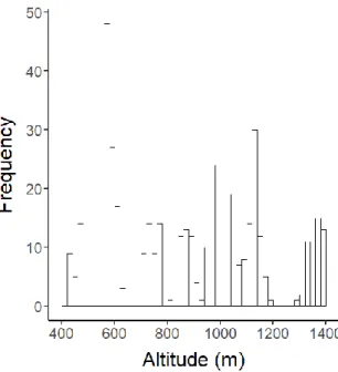
Figure 1.1: Frequency of nest boxes situated along the altitudinal gradient (50 m intervals). ……….……… 37
Chapter Two: Extreme plasticity in breeding phenology across an altitudinal gradient: implications for understanding phenological mismatch
Figure 2.1a: Relationship between average daily temperature (°C) and Julian date (100 = 10st April in non-leap years/ = 9th April in leap years) per altitudinal category. ………..……… 54
Figure 2.1b: Relationship between Julian lay date (100 = 10st April in non-leap years/ = 9th April in leap years) and altitude (m) (N = 536). Vertical, dashed lines indicate the cut-offs for the altitudinal categories. The best-fit lines are given per year. ……...……….. 54
Table 2.1: Lay date characteristics per altitudinal category (low, mid and high) and per year (2012-2017). ……… 55
11
Figure 2.2a: Relationship between the number of eggs laid and Julian lay date per altitudinal category – low: black points, mid: grey points, high: hollow points. Predictive lines controlling for year per altitudinal category - low: full, mid: dashed, high: dotted line (GLM with normal Gaussian error structure; N = 466). ……….……….. 57
Figure 2.2b: Relationship between the number of eggs and year (2012-2017; N = 466). ……….……….……… 57
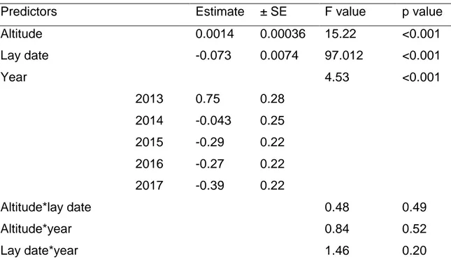
Table 2.2: Model summaries predicting clutch size. Linear model with normal error structure. ……… 58
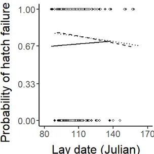
Figure 2.2c: Relationship between the probability of hatch failure and Julian lay date, per year: Predictive lines controlling for the number of eggs incubated and altitude (GLM with binomial error structure; N = 479). ………...……….. 60
Figure 2.2d: Relationship between the probability of hatch failure and Julian lay date per altitudinal category – low: black points, mid: grey points, high: hollow points. Predictive lines controlling for the number of eggs incubated and year per altitudinal category - low: full, mid: dashed, high: dotted line (GLM with binomial error structure; N = 479). ……….………. 60
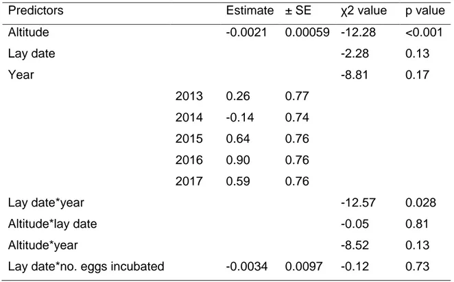
Table 2.3: Model summaries predicting the probability of hatch failure. Binomial GLM with logit link. ………….……… 61
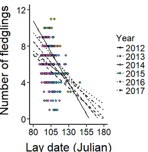
Figure 2.3a: Relationship between the probability of fledging and Julian lay date, per year: Predictive lines controlling for altitude (GLM with binomial error structure; N = 439). ……… 63
Figure 2.3b: Relationship between the probability of fledging and Julian lay date per altitudinal category – low: black points, mid: grey points, high: hollow points. Presented are best-fit lines (minimal model only included altitude) per altitudinal category - low: full, mid: dashed, high: dotted line (GLM with binomial error structure; N = 439). ……… 63
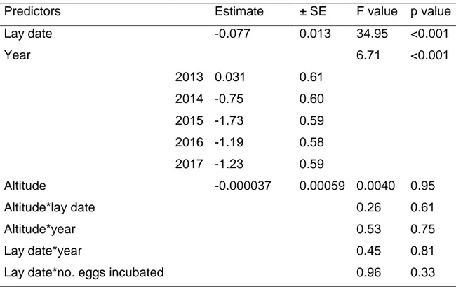
Table 2.4: Model summaries predicting the probability of fledging. Binomial GLM with logit link. ……….……… 64
Figure 2.3c: Relationship between the total number of fledging and Julian lay date, per altitudinal category – low: black points, mid: grey points, high: hollow points. Predictive lines controlling for year per altitudinal category - low: full, mid: dashed, high: dotted line (GLM with normal error structure; N = 369). … 66
Figure 2.3d: Relationship between the number of fledging and Julian lay date, per year: Predictive lines controlling for altitude (GLM with normal error structure; N = 369). ……… 66
Table 2.5: Model summaries predicting the total number of fledging. Linear model with normal error structure. ..……… 67
13
Figure 2.4: Relationship between average chick mass per brood (g) and Julian lay date, per clutch size category – small: white points, medium: grey points, large: small points. Predictive lines controlling for linear brood age, altitude and year per altitudinal category - small: full, medium: dashed, large: dotted line (GLM with normal error structure; N = 347). ……..……… 69
Table 2.6: Model summaries predicting average chick mass per brood. Linear model with normal error structure. ………..……… 70
Chapter Three: Testing the use of budburst as a reliable cue to breeding phenology in a population of blue tits breeding along an altitudinal gradient
Table 3.1: Characteristics of budburst date and lay date and temperature over the study period (2013-2017) with altitude. …..………. 89
Figure 3.1: Budburst date (Julian: 100 = 10st April in non-leap years/ = 9th April in leap years) with average daily temperature (°C) over the budburst period per altitude category. The points are annual measures. …………...………. 90
Figure 3.2: The delay to laying after budburst (d) in relation to altitude (m; F1,439 = 8.97, P = 0.0029). Raw data points and predictive line controlling for year... 90
Figure 3.3: Variance in lay date with variance in budburst date per altitude category. The points are annual measures. ………..……… 91
Figure 3.4: The probability of laying gaps occurring in relation to the delay in laying after budburst (d; χ21,362 = 1.86, P = 0.17) – low: black points, mid: grey
points, high: hollow points. Predictive lines controlling for year, per altitudinal category - low: full, mid: dashed, high: dotted line. ……….. 93
Figure 3.5: The delay to incubation after clutch completion (d) in relation to the delay in laying after budburst (d; F1,350 = 8.25, P < 0.0043) – low: black points, mid: grey points, high: hollow points. Predictive lines controlling for the length of the laying period and year, per altitudinal category - low: full, mid: dashed, high: dotted line. ………...……… 95
Figure 3.6: The length of the incubation period (d) in relation to the delay in laying after budburst (d; F1,378 = 3.72, P = 0.0543) – low: black points, mid: grey points, high: hollow points. Predictive lines controlling for the length of the pre-incubation period, the number of eggs incubated and year, per altitudinal category - low: full, mid: dashed, high: dotted line. ……….. 97
Figure 3.7: The length of the rearing period (d) in relation to the delay in laying after budburst (d; F1,310 = 4.30, P = 0.039) – low: black points, mid: grey points, high: hollow points. Predictive lines controlling for year, per altitudinal category - low: full, mid: dashed, high: dotted line. …….……… 99
15
Figure 3.8: The number of fledglings in relation to the delay in laying after budburst (d; χ2
1 = 2.65, P = 0.27) – low: black points, mid: grey points, high:
hollow points. Predictive lines controlling for year, per altitudinal category - low: full, mid: dashed, high: dotted line. ………..………. 101
Chapter Four: Inducing females to lay more eggs leads to increased per
capita provisioning rates of nestlings in blue tits
Figure 4.1: The average number of eggs laid in control versus experimental treatments after controlling for lay date, altitude and year (F1,45 = 32.75, P < 0.0001). Shown are the predicted mean ± SE. ………...…… 118
Figure 4.2: The relationship between control and experimental treatment group and a) average egg volume per clutch (χ21,27 = -0.0072, P = 0.39, b) the number
of eggs incubated (χ21,45 = -0.0016, P = 0.97), c) the number of hatchlings (F1,47
= 0.23, P = 0.64) and d) hatching synchrony (χ21,21 < -0.005, P = 0.91), after
controlling for lay date, altitude and year where relevant, plus the number of eggs laid for the average egg volume per clutch and the number of eggs incubated for the number of hatchlings. Shown are the predicted mean ± SE. ………. 120
Figure 4.3: Hourly feeding rates of females (full line) and males (dotted), in relation to brood size, controlling for the number of eggs laid, linear brood age, lay date and year (χ22,47 = 43.72, P < 0.001). Shown are the predicted lines of
best fit and raw data points for females (filled circles) and males (hollow circles). ……….… 122
Figure 4.4: Hourly feeding rates of females (filled circles) and males (hollow circles), in relation to control and experimental treatment (females - F1,43 = 9.13,
P = 0.004; males - F1,43 = 2.87, P = 0.098), controlling for the squared effect of brood size, linear brood age, lay date and year. Shown are the predicted mean ± SE. ………..………… 124
Figure 4.5: Hourly feeding rates of females (full line) and males (dotted), in relation to the number of eggs laid (controlling for the squared effect of brood size, linear brood age, lay date and year; χ21,46 = 3.13, P = 0.077). Shown are
the predicted lines of best fit and raw data points for females (filled circles) and males (hollow circles). ……….……… 126
17
Chapter Five: Brood size manipulations across an altitudinal gradient shed new light on investment strategies in a bi-parental care system
Figure 5.1: Hourly feeding rates of females (full line) and males (dotdashed; main effect of sex - χ21 = 11.61, P < 0.001), in relation to (a) natural brood size
(controlling for the proportion of caterpillars delivered and the random factor of nest box identity; main effect of natural brood size - χ21 = 7.29, P = 0.009; brood
size * sex interaction - χ21 = 1.90, P = 0.17); and (b) altitude (m; controlling for
linear and squared brood size, the proportion of caterpillars delivered and the random factor of nest box identity; main effect of altitude - χ21 = 2.072, P = 0.15;
altitude * sex interaction - χ21 = 2.85, P = 0.091). Shown are the predicted lines
of best fit and raw data points for females (filled circles) and males (hollow circles). …….………. 151
Table 5.1: Model summaries predicting provisioning rate / h, from linear mixed models including nest box ID as random effect. ……… 152
Figure 5.2: Differences in hourly feeding rates of males minus females, in relation to: (a) brood size (controlling for altitude; linear effect - F1,93 = 2.035, P = 0.16; quadratic effect - F1,92 < 0.001, P = 0.98); and (b) altitude (m; not controlling for other covariates - F1,94 = 3.72, P = 0.057). Shown are the predicted lines of best fit and raw data points. ……….. 154
Figure 5.3: Hourly feeding rates in relation to treatment groups (χ22 = 81.78, P <
0.001). The fixed covariates altitude, original linear brood size and proportion of caterpillars delivered are controlled for, in addition to the random factor of nest
box identity. These covariates were taken from the minimal models. Shown are the predicted mean ± SE. ………..………. 156
Table 5.2: Model summaries predicting provisioning rate / h, from linear mixed models including nest box ID as random effect. ………. 157
Figure 5.4: Differences in total hourly feeding rates of treatments minus combined controls (χ21 = 19.65, P < 0.001). The fixed covariate altitude is
controlled for, in addition to the random factor of nest box identity. This covariate was taken from the minimal models. Shown are the predicted mean ± SE. …………..……… 159
Figure 5.5: Differences in hourly feeding rates of treatments minus combined controls, a) per sex (main sex effect: χ21 = 3.11, P = 0.078; treatment * sex
effect: χ21 = 7.00, P = 0.0082), b) per altitudinal category (main altitude effect:
χ21 = 6.26, P = 0.012; treatment * altitude effect: χ21 = 0.38, P = 0.54). The
boxplots are plotted from raw data. ……….………. 161
Figure 5.6: Mean chick mass per brood (g) in relation to treatment groups. The fixed covariates altitude, original linear brood size, squared brood age and date are controlled for, in addition to the random factor of nest box identity (χ22 =
29.93, P < 0.0001). Shown are the predicted mean ± SE. ……… 163
Figure 5.7: Differences in mean brood mass (g) of treatments minus combined controls (χ21 = 15.95, P < 0.001). The boxplots are plotted from raw data. ... 163
19
Eurasian blue tit (Cyanistes caeruleus, Linnaeus 1758) The study species being characteristically aggressive when caught.
Chapter One
21
1.1 General framework
A key area and driver of evolutionary biology is how animals, including humans, invest in reproduction due to the potent influence on individuals’ fitness. Reproductive or parental investment is defined as “any investment by the parent
in an individual offspring that increases the offspring’s chance of surviving (and hence reproductive success) at the cost of the parent’s ability to invest in other offspring” (Trivers 1972) and other fitness contributors such as parental survival
and growth (Clutton-Brock 1991). Reproductive investment is integral to species‘ life histories (Stearns 1992), particularly as animals must balance the cost and benefit of reproduction to maximise life-time fitness (Williams 1966). Studies of parental investment have thus the potential to greatly enhance our understanding of underlying mechanisms driving evolutionary processes. In the following, I will highlight the historical origins of the concepts of reproductive investment and parental care, different parental care systems, existing gaps in our understanding of the forms and maintenance of bi-parental care today and which of these gaps I will address in this PhD thesis, along with the methodology to do so.
1.1.1 Reproductive investment
Surprisingly, even though key to species’ life histories, the field of reproductive investment is less than a century old. In the 1930s, Ronald Fisher was one of the first to acknowledge its importance in shaping natural selection in his book entitled “The Genetical Theory of Natural Selection”, built on the works of Charles Darwin and the founder of modern genetics; Gregor Mendel. Fisher was a pioneer in highlighting that reproductive investment should vary depending on the expected current and future fitness returns (Fisher 1930; Roff
1992; Stearns 1992; Houston and McNamara 1999). Further, Angus Bateman (1948) developed a principle in fruit flies (Drosophila melanogaster) that stated that lower reproductive variance should be found in females than males as their reproductive success does not benefit from a larger number of mates, but also that females invest more in offspring and are in turn more important for offspring’s’ reproductive success than males. Later, a theoretical model by C. Smith and Fretwell (1974) demonstrated that investment in offspring number and quality is inversely related, and that higher investment leads to greater offspring fitness. Around this time, Robert Trivers also explored reproductive investment based on human sexual behaviour in the book “Parental investment
and sexual selection” (1972). Trivers expanded on Bateman‘s principle showing
a difference in reproductive investment between the sexes; with females investing higher in the production of eggs than males invested in sperm and thus being key to sexual selection. This was in stark contrast to Fisher’s idea that the cost of reproductive investment should be the same between the sexes (Fisher 1930). In support of Bateman’s and Trivers’ arguments, parental care (a form of reproductive investment) exhibits unequal costs and responsibilities between the sexes (Kokko and Jennions 2008; Klug et al. 2013).
1.1.2 Parental care
Parental care was first defined by Clutton-Brock (1991) as “any form of parental
behaviour that appears likely to increase the fitness of a parent’s offspring”.
However, in this thesis I use a more specific, updated definition of parental care proposed by Royle and colleagues (2012) as being “parental behaviour that 1)
occurs post-fertilization (or after the production of daughter cells if reproduction is asexual), 2) is directed at offspring, and 3) appears likely to increase offspring
23
lifetime reproductive success”. Thus, behaviours that have possibly not evolved
to increase offspring fitness are excluded from this latter definition.
Parental care is rare, though can be found in diverse forms across the animal kingdom (Clutton-Brock 1991; Alonzo 2010; Royle et al. 2012). Parental care ranges from simply provisioning gametes with one-off nutrient transfers or selecting optimal sites for oviposition to more sophisticated parent-offspring interactions such as food provisioning after birth (Royle et al. 2012). Such parental care can last for extensive periods; for example in mammals young are often tended for until and past entering adulthood (Gubernick 2013). In humans this parental care period is exceptionally long for primates – up to 20 years (Howell 1979; Hawkes et al. 1998; Hill and Kaplan 1999). Amphibians such as alpine salamanders (Salamandra lanzai) also have a relatively long dependency period with young spending up to four years in utero (Miaud et al. 2001). In general, offspring will benefit from a longer duration of parental care, however this will also prevent parents from reproducing again sooner rather than later (Trivers 1972; Maynard Smith 1977; Clutton-Brock and Vincent 1991). Thus, parental care clearly carries costs. In extreme cases such as social spiders (Stegodyphus dumicola), the mother sacrifices her body to be eaten by the offspring – a process called matriphagy (Junghanns et al. 2017). This matriphagy occurs after the female has invested multiply in egg production, egg sac tending and regurgitation feeding. This example illustrates that parental investment decisions must be made at different stages of a breeding attempt to minimise reproductive costs.
Trade-offs between current versus future reproductive investment choices have been demonstrated (Tinbergen and Both 1999, and references within). For example, in burying beetles (Nicrophorus orbicollis) those females experimentally forced to produce more offspring experienced lower lifetime fecundity and died at a younger age than controls (Creighton et al. 2009). Females, which were given larger carcasses to raise their young on, also invest higher in current than future reproduction. Contrastingly, less attention has been paid to trade-offs in parental care between different time points of one breeding attempt. These intra-seasonal trade-offs may however be crucial for our understanding of overall life history strategies. The few empirical studies to date have focused on long-lived bird species such as common terns (Sterna hirundo; Heaney and Monaghan, 1995) and lesser black-backed gull (Larus fuscus; Monaghan et al., 1998). Negative trade-offs between stages of a single breeding attempt were found in these studies. For instance, in the lesser black-backed gull study females that were induced to lay an additional egg, though obtained the same number of chicks as controls, reared these at a lower rearing quality and thus had lighter chicks. However, more short-lived species should invest higher in a current breeding attempt than long-lived species, as their future reproductive chances (residual reproductive value) are lower, leading to possible diverging results than those found in long-lived species (Stearns 1992). To my knowledge, no empirical studies so far have directly tested these trade-offs within a breeding attempt in short-lived species (though see evidence of additive female fitness consequences in Visser and Lessells, 2001). Furthermore, early high investment by one partner, such as mothers having to produce the offspring, may impact other caregivers such as fathers at later
25
stages of rearing, adding another facet to the story (Russell et al. 2007, 2008; Savage et al. 2013).
1.1.3 Systems of parental care
Offspring can be reared by differing number of caregivers and this has consequences for their fitness and that of the caregivers (Clutton-Brock 1991). On one side of the care spectrum, a single parent is solely responsible for rearing young. For instance, paternal care is common in fish performing care (Klug et al. 2013). In black-striped pipefish (Syngnathus abaster), males carry the entire cost of pregnancy by brooding the eggs until hatching, leading to sex-role-reversal (Wilson et al. 2001; Cunha et al. 2017). In invertebrates and mammals, maternal care can be more frequently found (Klug et al. 2013). Maternal care is obligatory in mammals, as the offspring are dependent on milk produced by the mother after birth (Royle et al. 2012). However, at the other extreme a small minority of mammals and birds perform cooperative breeding (Cockburn 2006; Lukas and Clutton-Brock 2013); where caregivers other than the genetic parents help raise the offspring (Royle et al. 2012). In eusocial insect systems such as honey bees (genus Apis) cooperative breeding can even lead to sterilisation of some individuals in the social group (Naeger et al. 2013). Central on the spectrum lies bi-parental care. A tenth of mammal species fall into this care system (Reynolds et al. 2002), with male contribution being shown to increase litter size, decrease female lactation period and thus enable more frequent breeding (West and Capellini, 2016; though also see (Stockley and Hobson 2016). Around 80 % of extant bird species perform bi-parental care (Kendeigh 1952; Cockburn 2006).
Bi-parental care leads to a fascinating interplay between conflict and cooperation as two unrelated individuals together raise genetic offspring. Each member benefits from minimising their investment cost and taking advantage of their partner working harder in rearing (Trivers 1972). This evolutionary “game” has gripped the attention of many theoreticians over the last 40 years. Starting in the 1980s, Houston and Davies developed a ‘sealed bid’ model, where parents invested at a fixed level after making a single choice in investment (1985; also see Chase, 1980). These theoreticians built on previous models of genetically fixed parental investment (Maynard Smith 1977), though instead viewed parental care as a facultative behavioural reaction (Chase 1980). They found that the evolutionary stable strategy (ESS) was partial compensation, predicting that any change in one parent’s care level will be matched by the partner partially. For example, if a female drops her feeding rate the male will increase his rate, though insufficiently to match the original total provisioning level. This strategy should limit the occurrence of cheating at the population level. McNamara and colleagues (1999) updated these early bi-parental models by incorporating negotiation at different points during rearing. Thus, the partners respond directly to each other’s efforts. Partial compensation was again found to be the ESS. Average results of a meta-analysis of 54 bird empirical studies support this theoretical ESS, though many exceptions exist (Harrison et al. 2009). One explanation for these exceptions may be that parents match each other’s care levels when an asynchrony in information levels exists between the sexes (Hinde 2006; Johnstone and Hinde 2006; Meade et al. 2011). Thus, the parent with less information may use their partner’s rearing effort as a sign of brood demand and thus match their effort. Another explanation for deviations from traditional predictions may be that most classic models do not consider
27
how environmental variation may affects the cost and benefit of parental investment and thus cooperation between the sexes over offspring care.
1.1.4 Environmental variation
One of the first parental investment models incorporating environmental variation found that under higher variability parental fitness should benefit from investing equally in each offspring (McGinley et al. 1987). However, empirical studies often find a large variation in offspring sizes in more variable environments, maybe due to developmental constraints such as maturation rate. In harsher, more heterogenous conditions life history theory predicts that parents should invest higher into each offspring to increase their survival chances, rather than into producing more offspring (Smith and Fretwell 1974; Lloyd 1987; Stearns 1992). In support of this, Atlantic salmon (Salmo salar) show a conservative bet-hedging by producing less but higher quality offspring in such variable environments (Einum and Fleming 2004). These reproductive investment strategies may be part of a larger pace of life strategy characterising species’ life histories, which is dependent on environmental conditions (MacArthur and Wilson 1967; Wilbur et al. 1974; Stearns 1976, 1977; Ellis et al. 2009). It was shown in the erpobdellid leech (Nephelopsi obscura), that lower environmental predictability such as in temperature, led to higher mortality risk and plasticity, with individuals flexibly shifting their reproductive investment strategy along the pace of life gradient to match their environment (Baird et al. 1986). Specifically, a slow pace of life is characterised by longer developmental periods, lower reproductive rates, though higher levels of parental care to increase offspring recruitment and life expectancy in more variable environments (Gaillard et al. 1989; Ricklefs and Wikelski 2002; Réale et al.
2010). In support, heightened parental care has been found to increase fitness in more variable environments (Bonsall and Klug 2011).
The effect of environmental variation on parental investment is of particular interest under current climate change. Climate change is leading to increases in global temperature and variance of weather patterns including a growing record of exceptional climatic events (Intergovernmental Panel on Climate Change 2014). These two effects combined are having an impact on key reproductive investment decisions (Parmesan 2006). For example, species are shifting offspring production to match optimum environmental conditions; which has been recorded in a diverse array of taxa, presumably as an adaptive response to climatic changes (e.g. resident and migratory birds - Charmantier et al. 2008; Hüppop and Hüppop 2011; fish - Crozier and Hutchings 2014; insects - Andrew et al. 2013; amphibians and reptiles – Urban et al., 2014; though see Lyon et al., 2008). These shifts may be viewed as parental effects, by which mothers and fathers, through their own capacity to plastically invest in offspring, might be able to generate early, non-genetic channels, such as the hormonal content of eggs or nesting site choices, which inform the next generation before or soon after birth of prevailing environmental conditions (Cheverud and Moore 1994; Badyaev and Uller 2009; Wolf and Wade 2009). These maternal effects might hasten the speed of evolution by generating offspring plastically suited to their environment (Mousseau et al. 2009); though the reverse may also be true by shielding genotypes from selection (Räsänen and Kruuk 2007) - the debate is still ongoing. The direct knock-on effects of these parental mechanisms on population-level reproductive decisions and fitness in a changing climate have
29
been hard to decipher, as measuring climate change effects require decades of data collection.
Instead of longitudinal studies, more short-term, variable environmental systems may be used to understand climate change responses. Environmental gradients offer an opportunity to study the interaction between parental investment strategies and environmental harshness, and consequently its effect on reproductive fitness. Extreme, harsh environments may provide organisms with greater selective challenges, leading to a stronger role of phenotypic plasticity in reproductive strategies and further in directing species’ evolution (Rotkopf and Ovadia 2014). Some evidence comes from microbial communities, which live in extreme habitats (acid mine drainages, saline lakes or hot springs). These populations evolve faster than their counterparts in more lenient conditions (Li et al. 2014). Latitudinal gradients have been the norm to study environment-dependent life history trade-offs, mostly focusing on temperate north-south clines. Congruent with theory, female coho salmon (Oncorhynchus kisutch) lay less, though larger eggs to combat stronger competition for lower resources and increased predator risk at more southern latitudes (Fleming and Gross, 1990). Similar quantity-quality trade-offs have been demonstrated in various other taxa solely investing in eggs (Fox et al. 1997; Armbruster et al. 2001; Johnston and Leggett 2002; Khokhlova et al. 2014), and in species such as birds with more extensive parental care (Smith et al. 1989; Järvinen 1996; Encabo et al. 2002). However, much variation exists in the specific investment choices made and reproductive trade-offs may not only occur in a two-dimensional manner. For example, a meta-analysis looking at 135 different galliform species found that the typical increase in clutch size observed with latitude and thus seasonal
environments (Lack 1947; Jetz et al. 2008) may be confounded by an interaction with altitudinal gradients (Balasubramaniam and Rotenberry 2016).
Altitudinal gradients are a potent alternative proxy of climate change to latitudinal systems in investigating how parental investment strategies change with environmental variation. Compared to latitudinal gradients, they have smaller geographic ranges and thus minimise differences in day length and in genetic backgrounds of populations. More generally, montane environments constitute up to 25 % percent of the earth‘s surface, providing habitat for a vast amount of species (Meybeck et al. 2001; Spehn and Körner 2005). These environments are also one of the most vulnerable to climate change, leading to species range shifts, contractions and extinctions (Parmesan 2006; Sorte and Jetz 2010). Altitudinal gradients are characterised by drops in air temperature and oxygen levels, frequent extreme weather events such as sudden snow storms and summers being shorter with decreased plant and insect productivity, paralleling climate change (Rolland 2003; Körner 2007). These environmental changes affect species living at high altitudes (see review by Laiolo and Obeso, 2015). In plants, life history shifts have been found with altitude such as decreased body size, less investment into reproduction, though more into vegetal growth (Young et al. 2002; Hautier et al. 2009). Other examples come from animal taxa such as insects; grasshoppers (Omocestus viridulus) at high elevation have longer egg and juvenile developmental periods (Berner et al. 2004). In humans a shift to a slower pace of life has also been demonstrated; Andean Nuñoa women living above 4000 m have lower reproductive fitness and their children experience slower developmental time (Little and Baker 1976).
31
Birds invest greatly in reproduction with an extremely high prevalence of bi-parental care (80 %; Cockburn, 2006; Royle et al., 2012), leading to complex life history strategies. Phenotypic alterations with altitude have already been demonstrated in birds. Pre- and post-hatching parental investment, body fat levels and other morphological characteristics (e.g. wing length), and survival rates have been shown to change with altitude (Altshuler et al. 2004; Bears et al. 2009; Lu, Xin et al. 2011; Evans Ogden et al. 2012; Bastianelli et al. 2017). Empirical work points to a slower life history strategy, including longer developmental periods with altitude. In a meta-analysis of paired low versus high elevation bird population, Boyle and colleagues (2016) found that the annual number of breeding attempts and early investment (clutch size) consistently decreased with altitude. For example, the number of fledglings per female was halved in dark-eyed juncos (Junco hyemalis) breeding at high compared to geographically close low altitudinal sites, though higher offspring survival rates existed at higher altitudes (Bears et al. 2009). Across 24 pairs of avian species, Badyaev and Ghalambor (2001) showed that male contribution to nestling feeding increased with altitude, at the cost of sexual traits. However, Boyle et al.’s meta-analysis (2016) found much variation at later stages of reproductive attempts in parental care and survival, which does not conform to the traditional slow pace of life suggested for harsher montane environments. This may be due to evolutionary constraints such as slow generation times and range edges of species (Laiolo and Obeso 2015). Overall, our understanding of the underlying mechanisms and the role of avian parental investment decisions in life history evolution exhibit large gaps, in particular in the face of climate change.
1.2 PhD aims
The overall aim of this PhD is to investigate how parental investment strategies change with environmental harshness along an altitudinal gradient (a proxy for climate change) and what potential consequences this will have on fitness. In line with this, the overarching questions asked in this PhD are:
(a) Do parents, in particular mothers, change their reproductive investment depending on environmental harshness; i.e. along the altitudinal gradient? Does the altitudinal gradient highlight differences in investment strategies with the progression of the season? If so, do these changes in reproductive investment have consequences on reproductive output, specifically the quality and quantity of offspring? (Chapter Two)
(b) Do parents change their reproductive investment depending on environmental cues? In particular, do potential budburst cues play a role in adjustment of reproductive timing with food availability? (Chapter Three)
(c) Can reproductive investment choices be balanced across different time points of a breeding attempt? Are there potential links between early and late investment choices? (Chapter Four)
(d) How do bi-parental systems coordinate reproductive investment in line with changing reproductive costs such as environmental harshness and brood demand? (Chapter Five)
(e) How can reproductive investment and parental care models be improved with these new thesis findings? What hypothetical impacts do these reproductive investment choices have in a changing world? (Chapter Six)
33
1.3 Study species
I aim to investigate these question with a combination of observational and experimental studies. Specifically, I make use of a frequently used model organism, the Eurasian blue tit (Cyanistes caeruleus). The blue tit is a small cavity nesting, passerine bird occurring in the Western Palearctic (Föger and Pegoraro 2004). The IUCN redlist lists the blue tit as a least concern conservation status with large, even increasing populations sizes (BirdLife International 2016). It is a 12g passerine, blue and yellow in colour, with small sexual dimorphism (Föger and Pegoraro 2004). Preferred habitats for breeding are mixed deciduous forests as opposed to coniferous stands. Generally this species occurs in lowlands, but the record for breeding has been set at 3500 meters above sea level in the Caucasus mountain range (Cramp and Perrins 1993; Föger and Pegoraro 2004). This socially monogamous species has been thoroughly studied since the 1850s due to its wide distribution and accessible breeding in artificial nest boxes and large, manipulable clutch sizes (5-15 eggs; Krüper, 1853; Nur, 1986). In this species only the female builds nests and incubates the eggs, though both parents provision the chicks (Cramp and Perrins 1993). Thus, conveniently I can manipulate maternal investment strategies at the early stages in this model organism and also investigate parental costs for both parents at the rearing stage, plus test for partner responses.
1.4 Study system
Within my fieldwork, I utilise a novel 1000m altitudinal study system, located in the French Pyrenees mountain range. The French Pyrenees are characterised by relatively short, though steep valleys with mixed forests gradually turning into beech and fir stands above 900 m (Ninot et al. 2017). The tree line and the transition to mountain pastures is situated at ca. 1500 m, depending on the geological profile (Prodon et al. 2002). Additionally, since the second half of the 20th century, abandonment of land and farming practice is leading to increases in forested areas (Gibon and Balent 2005; Mottet et al. 2006). The focus population breeds in an established nest box population (N = ca. 640) across a 450-1500 m altitudinal gradient. I have aimed to distribute the nest boxes evenly across the altitudinal gradient, however due to characteristics of the terrain (e.g. steep slopes) some irregularities and minor gaps exist (Fig. 1.1). Woodcrete nest boxes were installed before the first breeding season in 2012 with a distance of more than 50 m between neighbouring boxes. In addition, handcrafted bamboo poles are used to lift down nest boxes. Nest boxes are shared with other passerine species; mainly great tits (Parus major), coal tits (Periparus ater), marsh tits (Poecile palustris), and occasionally nuthatches (Sitta europaea). A full characterisation of the study system can be found in Chapter Two.
35
Figure 1.1: Frequency of nest boxes situated along the altitudinal gradient (50 m intervals).
1.4 Thesis outline
The first data chapter (Chapter Two) will investigate general breeding parameters of our blue tit system. Specifically, I will investigate the associations among altitude, phenology, fecundity, productivity and nestling mass, from egg laying until fledging. Purely observational, climatic and reproductive data will be collated across six breeding seasons; including average daily temperature, clutch size, hatching and fledging numbers, fledging mass, and reproductive timing; i.e. first egg lay date. As part of characterisation of the altitudinal gradient, I will first investigate if average daily temperature shifts with elevation using temperature logger data. A gradual altitudinal decline in temperature is predicted (Körner 2007). Furthermore, lay date has been found to be closely linked to temperature, and further to phenology, i.e. tree and caterpillar development, which has consequences on later chick survival (McCleery and Perrins 1998; Sanz 2002). Thus, I predict that a delayed start of reproduction will be observed with increasing altitude, which should consequently affect later breeding parameters. Further, as the productive period is shorter at high altitude (Rolland 2003; Körner 2007), I predict that the reproductive output such as fledging numbers should be negatively affected. Specifically, I investigate phenological plasticity in response to altitude and year in this population. Second, I then investigate the effects of lay date and altitude on clutch size and hatching success, as a means of quantifying the phenotypic correlation between lay date and clutch size across the altitudinal gradient, and its effects on hatchability. Finally, I test the effects of lay date on fledging success and nestling mass to provide insights into phenological mismatch in this population, and whether such metrics of success are modified by phenology-fecundity associations.
37
The third chapter will look at if environmental cues such as budburst are used to differing degrees along the altitudinal gradient. As aforementioned, lay date has been found to be linked to phenology, i.e. tree development, which has consequences on later chick survival (McCleery and Perrins 1998; Sanz 2002). To investigate if females can predict optimal prey availability and thus if hatch date is correlated with this, budburst will be used as a proxy. As temperature is lower at higher altitudes (Körner 2007; Chapter Two), I predict budburst to be delayed compared to lowlands. This budburst should be tracked more closely by higher elevation birds as the season for reproducing in shortened, resulting in fewer reproductive opportunities. Thus, correct reproductive timing to exploit maximum environmental resources is crucial for reproductive success at high altitudes. To decipher this relationship, I will look at observational phenological and reproductive data, specifically at how well budburst and lay date is matched with altitude and whether this temporal relationship affects reproductive output such as fledgling numbers and mass. Additionally, I will investigate if strategies are used to improve the association between budburst and hatching after laying.
The fourth chapter will focus in on how parental investment choices are linked across different phases of a single breeding attempt. I will investigate how experimentally manipulated investment choices in early breeding phases (the number of eggs laid) will affect later investment levels at the rearing stage. The rationale behind this experiment is that most studies have ignored the costs of egg laying and incubation to females (Monaghan and Nager 1997). Both can contain a cost in various bird species, in particular for future fitness of the
female (Reid et al. 2000; Visser and Lessells 2001; Nager et al. 2001). These early costs should impact later investment in offspring (Savage et al. 2013), which should shift the care contributions of the parent directly affected (females), and their partner (males). However, these costs may also affect future reproductive abilities and especially in short-live species such as blue tits. Hypothetically, high early investment may lead to high investment at the rearing stage, as residual reproductive value is reduced if key resources are depleted faster and future survival is reduced (Stearns 1992). Thus, I predict that heightened, early invest by females will affect later investment choices in the rearing phase, however decreased and increased investment are possible. To test these two predictions, females are made to lay additional eggs, though incubation and rearing costs are kept constant, as in control groups, which were not made to lay additional eggs. This is achieved by a cross-fostering approach. Later investment in the rearing stage is investigated by observational data on provisioning of both parents.
The fifth chapter will concentrate on the rearing stage and highlight how different environmental drivers influencing parental care. In particular, I will look at if contributions of females and males change depending on altitude, year, caterpillar availability and intrinsic nest characteristics such as brood age and size. I predict that if environmental harshness (altitude) increases it will be harder for parents to provision at equivalent levels to their lowland counterparts. On the other hand, I predict that parents may respond in line with the pace of life framework, with high altitude individuals shifting to a slower pace resulting in higher parental care in fewer offspring (Hille and Cooper 2015; Boyle et al. 2016). Additionally, traditional theory does not consider differential task division
39
between the sexes, such as nest sanitisation by the female and predator defence task by the male (Maynard Smith 1977; Klug et al. 2013). This should result in differential investment strategies. As part of this, I will first explore natural nestling provisioning. As brood size is a key fitness trait, it must be a crucial factor for investment choices. However, the sexes may have different optimal brood sizes, depending on previous and future investment choices. Thus secondarily, a temporary brood manipulation is performed to reveal possible underlying differences in provisioning strategies between the sexes, in response to artificially increased or decreased brood sizes, compared to controls, and if responses change with altitude. I will test classic models of bi-parental care predicting: (a) comparable provisioning contributions of males and females independently of ecology; (b) partial compensation response rules by both sexes; and (c) these partial response rules to be manifest as overall increases in nestling mass.
Globally these observational and experimental data chapters aim to investigate underlying drivers and mechanisms of bi-parental care in birds. Reproductive costs of both parents during the pre- and post-hatching stages will be manipulated naturally with use of the altitudinal gradient and through directed experiments to investigate underlying reproductive strategies. To conclude, the sixth chapter will constitute an overall discussion aiming to tie all the results together found during this PhD. I aim to highlight the novelty these results for the field of parental care. I will be indicating overarching parental investment (care) strategies for this particular system. Impacts on potential species’ evolutionary processes and endurance under climate change prognoses will be discussed.
Chapter Two
Extreme plasticity in breeding phenology across an altitudinal
gradient: implications for understanding phenological
41
2.1 Abstract
There is a pressing need to understand whether and how populations respond to changing climates. To date, much of our understanding stems from longitudinal studies of sufficient duration to encapsulate climate shifts. While such studies provide essential insights, they obviously require significant time, and the magnitude of any effect measured is contingent upon the magnitude of inter-annual variation in climate; which is often modest. Here I use a 1000 m altitudinal gradient in the French Pyrenees to generate representative 2-3 °C differences in temperature faced by breeders in a population of blue tits (Cyanistes caeruleus). During the six years of study, I found that breeding phenology typically varied by ca. nine days within altitudinal zones, but was on average 11 days earlier at low versus high altitudes. Early breeding was generally associated with larger clutch sizes, which in conjunction with reduced nestling mortality, led to more young being fledged. However, compared with birds breeding at low elevation, those breeding at high elevations also laid larger clutches than expected for their lay dates. As a consequence, despite low elevation birds showing reduced probability of hatching failure compared with high elevation birds, they did not enjoy greater breeding success; and high elevation broods were also in better condition. Our results suggest that constraints on plasticity are unlikely to explain phenological mismatches; and lead us to hypothesise that the answer lies with the relative quickening of development of ectothermic prey with warming springs, compounded by current selection on negative phenology-fecundity associations of endothermic predators.
2.2 Introduction
Recent meta-analyses indicate that organisms of diverse taxonomy are responding to climate change by advancing the timing of key life events, particularly reproduction (Thackeray et al. 2010, 2016). Phenological responses within populations appear to be largely plastic (Phillimore et al. 2010), and such plasticity is suggested to play a significant role in allowing populations to adapt in real time to changing climate (Parmesan 2006; Both et al. 2006; Visser 2008; Both et al. 2009a; Visser et al. 2012; Gienapp et al. 2013). Nevertheless, whether plastic advances in breeding phenology are sufficient or adaptive will depend additionally on associated changes to reproductive investment, including fecundity and any subsequent levels of care. Despite this, less is known about potential constraints to plasticity or climatic impacts on adaptive associations among phenology, key life history traits and metrics of success (Visser et al. 2015; Visser 2016). In order to address these shortcomings, the obvious general association between the location of a population and its climate will often need to be de-coupled. There are two potential ways of achieving such decoupling in natural systems: intensive longitudinal study encapsulating sufficient climatic variation; and the use of altitudinal gradients to generate representative levels of climatic variation in the short term and to test responses by individuals from the same population in conjunction with their downstream consequences for investment and success.
Testing adaptive responses to climatic variation for fecundity and subsequent levels of care is more challenging than testing impacts on breeding phenology because fewer taxon are amenable to quantitative assessment of such measures. Birds offer an important model in this regard because fecundity and
43
subsequent care is variable and easily measured. Current evidence from longitudinal studies in such taxon, often spanning several decades, suggests that advancing lay date is generally often associated with increased clutch size (Potti 2009; Dunn & Møller 2014). This might be construed adaptive because the ability to advance breeding more in response to warming springs is likely to generate improved match with peaks in prey availability (Visser et al. 2006; Charmantier et al. 2008). On the other hand, higher fecundity generally leads to reductions in per capita prey acquisition rates, potentially compounding any effects of mismatches between phenology and prey availability. Interestingly, quantitative genetic approaches suggest a negative genetic correlation between phenology and fecundity (Sheldon et al. 2003), suggesting that an advance in lay date might often be associated with an incidental increase in clutch size. Compensating for increased clutch size as a consequence of advanced phenology would require increased parental effort, but whether or not this is the case is not well known (Dunn and Winkler 2010). Thus, it is currently unclear whether or not commonly reported negative associations between phenology and fecundity are adaptive, or contribute to documented detrimental effects of climate change (Dunn and Møller 2014).
While longitudinal studies are unquestionably invaluable, opportunities to establish such studies are now more limited and the time taken to do so is prohibitive with respect to the need for answers. A potentially viable alternative approach is to use altitudinal gradients to generate representative variation in climate among individuals within a single population. Altitudinal gradients have been commonly used to test for ecological impacts on key fitness-related traits. For example, a recent meta-analysis of bird species breeding across altitudinal
gradients showed that breeding phenology was considerably later at higher elevations, and that clutch sizes tended to be smaller (57 % of 98 species); with average reductions of ca. 6 % (Boyle et al. 2016). These finding mirror the results of longitudinal studies: that warmer weather leads to both advanced phenology and fecundity. However, almost all previous altitudinal studies have conducted comparisons of the same species across different populations, meaning that varying degrees of local adaptation could cloud assessment of plastic responses to climatic variation. In order to provide a more realistic analogy of climate change impacts, associations between phenology, fecundity, levels of care and productivity need to be investigated across altitudinal gradients within the same population.
Here I investigate the associations among altitude, phenology, fecundity, productivity and nestling mass in a nest box population of blue tits (Cyanistes
caeruleus) breeding along a 1000 m altitudinal gradient in the French Pyrenees.
This altitudinal range is associated an average 2-3 °C difference in mean daily (24 h) temperature during the breeding season. I am confident that any variation in parameters measures across our gradient is owed to plasticity because the median distance between sites is ~5 km, the habitat is contiguous between sites, and I have observed several instances of dispersal across our elevational gradient. The blue tit is a 12 g passerine in which the breeding female is responsible for all forms of care, and her male partner contributes to offspring provisioning. Previous longitudinal studies have suggested it to be able to advance lay date, plastically, in response to advancing springs, and to show associated increases in clutch size (Potti 2009; Ahola et al. 2009). However, generally no increased fledging success has been recorded with advancing
45
springs, suggesting that selection for larger clutches may be maladaptive due associated increasing costs of egg production and rearing, which may be enhanced due to a larger prey mismatch (Dunn 2004; Dunn and Winkler 2010).
Specifically, I first describe annual and altitudinal variation in breeding phenology as a means to investigate the maximal scope for phenological plasticity in this population. Second, I then investigate the effects of lay date and altitude on clutch size and hatching success, as a means of quantifying the phenotypic correlation between lay date and clutch size across the altitudinal gradient, and its effects on hatchability. Finally, I test the effects of lay date on fledging success and nestling mass to provide insights into phenological mismatch in this population, and whether such metrics of success are modified by phenology-fecundity associations.
2.3 Materials and Methods 2.3.1 Study population and habitat
Climate and reproductive data were collected near the research Station for Theoretical and Experimental Ecology of Moulis (SETE, UMR 5321; 42°57’29” N, 1°05’12” E), in the French Pyrenees during the breeding seasons of 2012-2017 inclusive. In total, our 14 woodlots contain on average 634 Woodcrete SchweglerTM 2M nest boxes (32 mm hole diameter) spaced at ca. 50 m intervals. The number of boxes per year ranged from 626 to 641. The mean distance between woodlots is 7.1 km (±5.1 SD; median = 5.2). The woodlots are connected by a contiguous mosaic of mixed deciduous woodland, primarily oak (Quercus robur), ash (Fraxinus excelsior) and hazel (Corylus avellana) and beech (Fagus sylvatica), with the latter tree species more common at higher elevations and the former at lower elevations. Temperature at three locations was obtained in three years: three loggers (TinytagTM types TGP-4500 and TGP-4505) were positioned in 2015 at 565, 847 and 1335 m elevation, set to 30 min interval readings. Daily (24 h) averages were created to estimate variation in diurnal and nocturnal temperatures. Work was conducted under animal care permits to A. S. Chaine from the French bird ringing office (CRBPO; n°13619), the state of Ariège animal experimentation review (Préfecture de l’Ariège, Protection des Populations, n°A09-4) and the Région Midi-Pyrenées (DIREN, n°2012-07).
2.3.2 Phenology, investment and success
We recorded data on lay date, clutch size, hatching failure and fledging success (all years). Each of these parameters was known with precision owing to nest checks every 3-5 days, or every day before the onset of laying, from the sixth
47
egg to clutch completion, at hatching and fledging, from day 11 of incubation and day 18 after chick hatching, respectively. Our blue tit population is single brooded, although pairs will have a second nesting attempt if the initial brood fails. No differentiation between first and any second attempts was made, as these could not be clearly distinguished due to the blurred overlap in lay dates correlated with the altitudinal cline (see below). The total number of hatchlings was determined as the number of eggs that hatched successfully, and the total number of fledglings as the number of chicks at banding (around day 15), minus those found dead after the rest of the brood flew the nest, as predation is rare in the late period of rearing (personal observation). Starting in 2013, all chicks were weighed to the nearest 0.05g (day 11-18 after hatching) using electronic scales. In addition, a unique metal ring was fitted to every chick.
Our full data set comprised 541 blue tit nests that laid a full clutch and for which I obtained the date of laying onset. However, the sample size is reduced in subsequent analyses, owing to rare cases of nest abandonment and the use of some nests in experiments for other purposes. For example, in 2013-14, 58 experimental nests were excluded from the clutch size analysis, as I modified egg laying in these nests (N = 483 remaining). However, this manipulation did not affect subsequent breeding parameters, since variation in the number of eggs incubated and hatchling numbers were controlled for through a cross-fostering approach (unpublished data). Nevertheless, 12 % of nests with zero hatchlings were excluded from the probability of hatch failure analysis (N = 479 remaining), since such cases appeared to be due to nest abandonment. Finally, from 2013, all chicks were weighed to the nearest 0.1 g (day 11-18 after hatching; N = 2249 nestlings, 347 broods).