Science Arts & Métiers (SAM)
is an open access repository that collects the work of Arts et Métiers Institute of Technology researchers and makes it freely available over the web where possible.
This is an author-deposited version published in: https://sam.ensam.eu
Handle ID: .http://hdl.handle.net/10985/7470
To cite this version :
Guillaume FROMENTIN, Gérard POULACHON - Geometrical analysis of thread milling – Part 1: Evaluation of tool angles The International Journal of Advanced Manufacturing Technology -Vol. 49, n°1, p.73-80 - 2010
1 2 3 4 5 6 7 8 9 10 11 12 13 14 15 16 17 18 19 20 21 22 23 24 25 26 27 28 29 30 31 32 33 34 35 36 37 38 39 40 41 42 43 44 45 46 47 48 49 50 51 52 53 54 55 56 57 58 59 60 61 62
Geometrical analysis of thread milling – Part
1: Evaluation of tool angles
G. Fromentin, G. Poulachon
Arts et Metiers ParisTech, LaBoMaP, 71250 Cluny, France
Email: guillaume.fromentin@cluny.ensam.fr Tel.: +33 3 85 59 53 30
Fax: +33 3 85 59 53 70
Keywords: thread milling, cutting geometry, tool angles
Abstract: Thread milling is a method which is increasingly used for machining thread. For this operation, a helical interpolation is required. Furthermore, the thread mill is a tool whose geometry is rather complex. Its envelope profile is linked to the thread profile and a single tooth of the thread mill is composed of three continuous cutting edges. The present study proposes a geometrical model and an analytical formulation to define the rake face and the cutting edge. Further, the calculations of cutting planes and cutting angles are explained. The analysis shows specific aspects of thread mills, in particular the fact that the flute angle may lead to a negative rake angle. This study is a contribution to cutting geometry aspect and constitutes a step for cutting force model in thread milling.
*Manuscript
1 2 3 4 5 6 7 8 9 10 11 12 13 14 15 16 17 18 19 20 21 22 23 24 25 26 27 28 29 30 31 32 33 34 35 36 37 38 39 40 41 42 43 44 45 46 47 48 49 50 51 52 53 54 55 56 57 58 59 60 61 62 NOMENCLATURE
Subscripts and abbreviations: m relative to the mill
r,z cylindrical coordinates fce: front cutting edge uce: upper cutting edge lce: lower cutting edge Referentials and parameters:
Ro = (o, e1,e2,e3) referential linked to the mill
zce: altitude of a cutting edge point in the Ro referential
u: parameter
Metric thread dimensions:
D: nominal diameter of the internal thread D1: minor diameter of the internal thread
D2: pitch diameter of the internal thread
H: fundamental triangle height P: thread pitch (mm)
p: angular thread pitch (mm/rad) Mill dimensions:
Dm: maximum diameter (mm)
D2m: pitch diameter (mm)
km: reduction coefficient of the mill profile height
pfm: pitch per radian of the helicoidal flute
Mill cutting angle:
om: orthogonal rake angle
sm: flute angle (or helix angle) on the Dm diameter
i: rake angle in Pi plane (i {n,f ,o,s} )
s: cutting edge inclination angle
r: cutting edge angle
Pr: tool reference plane
Ps: tool cutting edge plane
Pn: tool cutting edge normal plane
Pf: tool working plane
Po: tool orthogonal plane
TVce(zce): tangential vector with respect to CE1
TVce.Pr(zce): tangential vector with respect to CE1 projected onto plane Pr
1 2 3 4 5 6 7 8 9 10 11 12 13 14 15 16 17 18 19 20 21 22 23 24 25 26 27 28 29 30 31 32 33 34 35 36 37 38 39 40 41 42 43 44 45 46 47 48 49 50 51 52 53 54 55 56 57 58 59 60 61 62
NVPi(zce): normal vector with respect to the Pi plane (i {n,f ,o,s} )
Pr Pi
V : vector of the intersection of plane Pr and plane Pi
RF Pi
V : vector of the intersection of the rake face and plane Pi
Pr.Pi
NV : normal vector with respect to plane Pr projected onto plane Pi
RF.Pi
NV : normal vector with respect to the rake face projected onto plane Pi RV: radius vector
Cutting parameters:
rdoc: radial depth of cut (mm)
rp: radial penetration (mm)
Geometrical objects:
Pm i: ith characteristic point of the mill profile MP(zce): mill profile
RF(r,zce): mill rake face (flute surface)
CE(zce): mill cutting edge
Operators: R(): rotating operator cos( ) sin( ) 0 ( ) sin( ) cos( ) 0 0 0 1 R N(V): normative operator N V( ) 1 V V
1 2 3 4 5 6 7 8 9 10 11 12 13 14 15 16 17 18 19 20 21 22 23 24 25 26 27 28 29 30 31 32 33 34 35 36 37 38 39 40 41 42 43 44 45 46 47 48 49 50 51 52 53 54 55 56 57 58 59 60 61 62
1 Introduction
1.1 Generalities on thread milling
Threads can be produced by many methods among them, there is the thread milling technique. The description on thread milling cycle is given in [1,2]. This technique allows to machine both internal and external thread, and one mill may produce threads with different diameters and having same pitch. Torque is lower and cutting speed may be greater in thread milling than in tapping, and if tool breakage occurs, as the thread mill is having a lower diameter than internal thread, it can be removed easily. As a consequence, thread milling is well adapted to obtain internal thread, large thread dimensions, especially in high cost parts machining which may be done in difficult to cut materials. Further, application of thread milling is increasing in industry [3,4].
1.2 Tool and cutting geometry aspects
A thread mill is a rotating cutting tool with grooves, its profile is composed of the threaded one, and its envelope is a revolution surface. During the thread milling cycle, the tool center strategy describes a circular helix. This results in complex geometrical problems.
The first is how to design such cutting tool and which cutting geometry is adapted for machining. Concerning the groove is usually defined as being a helical.
The second is how to grind the thread mill from the CAD design. The definition of the grinding wheel profile used for the groove machining is a specific problematic due to inference problem [5-9]. This aspect of groove obtaining is also common to cylindrical mill manufacturing. Furthermore, the thread mill profile is fixed by the threaded and the grinding of
clearance surfaces is a difficult operation which is linked both from the groove positions and from the mill profile. This point is not dealt in earlier study.
Then, from this process it appears a third problem, which is the cutting ability of the mill in relationship with tool angles which are not constant along cutting edges.
For different kinds of tools, like fluted drills, taps, round insert cutters and also thread mills, there are evolutions of tool angles, in hand and/or in used, along the cutting edges. The tool angles can not be directly
determined from tool design and the cutting edge definitions. There exist different approaches [10,11] for establishing these tools angles. From this analysis, it is possible to improve the tool design and adapt cutting edge definition in order to minimize rake angle evolution or avoid large negative rake angle. This approach is needed as the rake angle affects cutting forces, tool chip friction, dead metal zone [12-14] and then cutting stability and tool wear [15].
1.3 Approach for the study
The complex problem of force modeling in thread milling has been started to be explored [1] and cutting angles are an interesting field for this
1 2 3 4 5 6 7 8 9 10 11 12 13 14 15 16 17 18 19 20 21 22 23 24 25 26 27 28 29 30 31 32 33 34 35 36 37 38 39 40 41 42 43 44 45 46 47 48 49 50 51 52 53 54 55 56 57 58 59 60 61 62
development. Better model needs to take into account the real cutting geometry at every point on cutting edge, because it significantly influences cutting forces and specific cutting energy [12-14].
The tool angle evolution on thread mill has not been dealt and a vectorial approach is proposed to investigate this case. The present study deals with the analysis of the cutting geometry of a thread mill having a straight or helical flute. The approach is explained in Fig. 1. The goal of this paper is to parameterize analytically a rake face (RF) and its associated cutting edge (CE) to calculate the tool angles.
This article is related to [2] and the general context is identical. A metric thread mill is considered, and the notation and Ro mill referential used are
the same as in [2]. All calculations are computed using Mathematica software. The parameterization of the thread mill operation is proposed in Fig. 2. For the different cases studied, the common mill dimension values are: Dm = 12 mm, P = 2 mm, km = 1/8.
2 Mill parameterization
This section describes the parameterization of the mill profile (MP), the rake face (RF) surface and the cutting edge (CE).
2.1 Mill profile
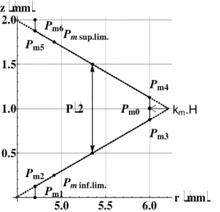
The mill profile (MP) is resulting from the thread profile [16]. The used mill profile (MP) is shown in Fig. 3, and it is defined by equation (1) [2] as a function of zce axial coordinate. The maximum diameter of the mill is
defined by Dm and its pitch by P. The crest of the mill is defined by a
reduction coefficient for the mill profile height called km. As explained in [2],
the mill profile is not completely engaged with the thread. The lower cutting edge (lce) works between the Pm inf.lim. and Pm3 mill profile points.
Symmetrically, the upper cutting edge (uce) works between the Pm4 and
Pm sup.lim. mill profile points.
T ce r ce ce
(z ) MP (z ), z
MP [ ] (1)
2.2 Rake face parameterization
It is decided to model the mill flute as being a helicoid. The pitch per radian (pfm) of this helicoid is defined by the flute angle (sm) on the
maximum diameter (Dm). The expression of this pitch is given by (2).
fm m sm
1
p D .tan( /2 - )
2
(2)
In addition to the flute angle (sm) on the circular helix enveloping the
thread mill, the orthogonal rake angle (om) on the maximum diameter (Dm)
is defined. From these tool angles, we obtain the VRF1 vector (3), included
in the rake face (RF), and the VRF2 vector (4), which is tangent to this
circular helix. T om om cos( ), sin( ), 0 [ ] RF1 V (3) T sm sm 0, sin( ), cos( ) [ ] RF2 V (4)
1 2 3 4 5 6 7 8 9 10 11 12 13 14 15 16 17 18 19 20 21 22 23 24 25 26 27 28 29 30 31 32 33 34 35 36 37 38 39 40 41 42 43 44 45 46 47 48 49 50 51 52 53 54 55 56 57 58 59 60 61 62
From the centre point of the mill profile (Pm0), the expression for the
generative line of the rake face (GLRF) is (5). The u parameter is the distance from point Pm0, and is an angular parameter. The rake face
(RF), which is considered as being a helicoid, can be parameterized by equation (6) according to [8,9]. T m (u) D / 2, 0, P / 2 u. RF GL [ ] VRF1 (5) T fm (u, ) 0, 0, p . ( ). RF(u) RF [ ] R GL (6)
In order to use cylindrical parameters, relation (7) is calculated, connecting the radial coordinate and the u parameter. The axial coordinate zce is
linked with the angular parameter (8). By using these parameter changes, a new analytical parameterization (9) of the rake face (RF) is established. 2 2 2 2 2 m om m m om r = (u, ). ) (u, ). ) 1
u(r) D .cos( ) r² D / 8 D cos(2. ) / 8 2 (RF e1 (RF e2 (7) fm ce p . z P / 2 (8) T ce ce ce fm (z , r) 0, 0, z P / 2 ((z P / 2) / p ). RF(u(r)) RF [ ] R GL (9)
Fig. 4 shows the mill profile (MP), the rake face (RF) and the geometrical construction of the cutting edge (CE).
2.3 Cutting edge parameterization
The cutting edge (CE) is the curve on the rake face (RF) surface which generates the same envelope as the mill profile (MP) when it rotates around the (o,e3) axis. Thus, the cutting edge (CE) can be expressed analytically by equation (10). The radial component of the mill profile (MPr)
is obtained by using the rake face (RF) equation (9) in cylindrical
coordinates. The cutting edge (CE), with characteristic points, is drawn in Fig. 5.
ce ce r ce
(z ) (z , MP (z ))
CE RF (10)
3 Cutting angle calculation
Definitions of tool planes and tool angles given by [17,18] are used. From the cutting edge parameterization, tool planes and tool angles may be calculated at every point of the cutting edge (CE). All geometrical
characteristics concern the tool-in-hand system. The various planes are defined only by unit vectors.
3.1 Cutting plane calculation
The reference plane (Pr) is defined as being normal to the cutting speed.
Thus, the normal vector to the reference plane (NVPr) may be expressed
1 2 3 4 5 6 7 8 9 10 11 12 13 14 15 16 17 18 19 20 21 22 23 24 25 26 27 28 29 30 31 32 33 34 35 36 37 38 39 40 41 42 43 44 45 46 47 48 49 50 51 52 53 54 55 56 57 58 59 60 61 62
T
Pr(z )ce (z )ce 0,0,1 NV N CE [ ] (11)The tangential vector of the cutting edge (TVCE) is calculated using
equation (12). Equation (13) gives the projection of this vector (TVCE.Pr) on
the reference plane (Pr).
ce CE ce ce (z ) (z ) z CE TV N (12)
CE.Pr(z )ce CE(z )ce CE(z ).ce Pr(z ) .ce Pr(z )ce TV N TV TV NV NV (13)The normal vector to the cutting edge normal plane (NVPn) is tangential to
the cutting edge (CE), and thus it is given by equation (14). The normal vector to the orthogonal plane (NVPo) is equal to the cutting edge
tangential vector projected onto the reference plane (TVCE.Pr). It is defined
by equation (15).
P n(z )ce CE(z )ce
NV TV (14)
Po(z )ce CE.Pr(z )ce
NV TV (15)
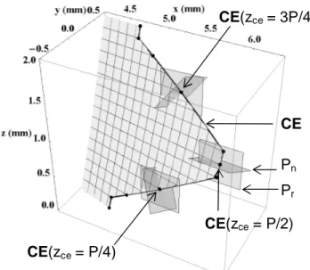
In Fig. 5 it can be seen that, at the cutting edge point altitude 3P/4, the rake face is in front of the reference plane (Pr) along the normal plane (Pn),
whereas this is not the case at the cutting edge point altitude P/4. That would mean the rake angle measured in this direction is negative on the upper cutting edge (uce).
The z axial component of the feed motion direction is not taken into
account because it is the tool-in-hand angles, and not the working angles, which are considered. Consequently, the normal vector to the working plane (NVPf) may be calculated using equation (16)
T P f(z )ce 0, 0,1
NV [ ] (16)
Concerning the cutting edge plane (Ps), it is normal to the reference plane
(Pr) and to the orthogonal plane (Po). Thus, its normal vector (NVPs) can be
calculated by equation (17)
Ps(z )ce Pr(z )ce Po(z )ce
NV NV NV (17)
A graphic representation of the cutting planes, on a point of the cutting edge, is given in Fig. 6.
Equation (18) gives the normal vector to the rake face (NVRF) at a cutting
edge (CE) point defined by zce altitude.
RF ce ce r ce ce r ce ce (z ) (z , MP (z )) (z , MP (z )) z r RF RF NV N (18)
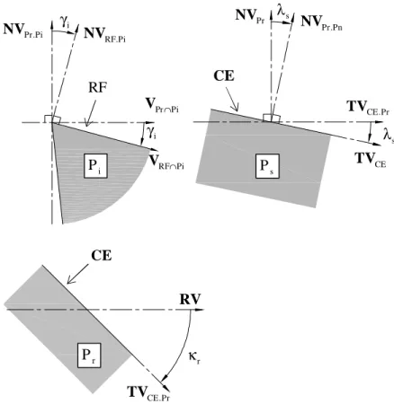
In order to calculate the cutting angle in the (Pi) plane (i {n,f,o,s}), it is
necessary to know the traces of different geometrical elements in this plane, as shown in Fig. 7.
Vector (VPr Pi ) of the line of intersection between reference plane (Pr) and
plane Pi can be calculated from equation (19). The normal vector (NVPr.Pi)
1 2 3 4 5 6 7 8 9 10 11 12 13 14 15 16 17 18 19 20 21 22 23 24 25 26 27 28 29 30 31 32 33 34 35 36 37 38 39 40 41 42 43 44 45 46 47 48 49 50 51 52 53 54 55 56 57 58 59 60 61 62
Pr Pi (z )ce Pr(z )ce Pi(z )ce i {n, f , o,s} V N NV NV (19)
Pr.Pi(z )ce Pr(z )ce Pr(z ).ce Pi(z ) .ce Pi(z )ce i {n, f , o} NV N NV NV NV NV (20)Vector (VRF Pi ) of the line of intersection between the rake face (RF) and
plane Pi can be calculated from equation (21). The normal vector (NVRF.Pi)
to the rake face (RF) projected onto plane Pi is given by equation (22).
RF Pi (z )ce RF(z )ce Pi(z )ce i {n, f , o} V N NV NV (21)
RF.Pi(z )ce RF(z )ce RF(z ).ce Pi(z ) .ce Pi(z )ce i {n, f , o} NV N NV NV NV NV (22)The radius vector (RV), defined by equation (23), is included in the reference plane (Pr).
T
ce ce ce
(z ) (z ). , (z ). ,0
RV = N [CE e1 CE e2 ] (23)
3.2 Cutting angle calculation
From the geometrical elements which are previously defined, as shown in Fig. 7, the rake angle, measured in plane (Pi), can be expressed by both
equations (24) and (25). It may be computed from the cross product and the dot product of the vectors. At point Pm0 of the cutting edge, the rake
angle (n(P/2)) in the normal plane is analytically given by equation (26).
i(z )ce RF Pi (z ),ce Pr Pi (z )ce V V (24)
i(z )ce RF.Pi(z ),ce Pr.Pi(z )ce NV NV (25) n 2 2 om sm 1 (P / 2) / 2 arccos 1 cot( ) .sec( ) (26)Angle s is the inclination of the cutting edge from the reference plane (Pr),
as shown in Fig. 7, and may be calculated using equations (27) or (28).
s(z )ce CE(z ),ce CE.Pr(z )ce TV TV (27)
s(z )ce Pr(z ),ce Pr.Pn(z )ce NV NV (28)The cutting edge angle (r) is the angle between the cutting edge (CE) and
the radius vector (RV) measured in the reference plane (Pr), as shown in
Fig. 7. It is expressed by equation (29).
r(z )ce CE.Pr(z ),ce (z )ce
TV RV (29)
4 CUTTING ANGLE ANALYSIS
This section details an example of cutting geometry analysis by using the developed approach on a given mill. Then, the approach is applied to
1 2 3 4 5 6 7 8 9 10 11 12 13 14 15 16 17 18 19 20 21 22 23 24 25 26 27 28 29 30 31 32 33 34 35 36 37 38 39 40 41 42 43 44 45 46 47 48 49 50 51 52 53 54 55 56 57 58 59 60 61 62
different mill geometries to observe the effects of flute angle (sm) and of
orthogonal rake angle (om) on normal rake angle (n).
4.1 Analysis of a thread mill angle
A thread mill is analysed (case A) with: Dm = 12 mm, P = 2 mm, km = 1/8,
om
= 10 °, sm= 30 °. Fig. 8 shows the evolution of the cutting angles along the cutting edge (CE). All cutting angles are constant on the front cutting edge, because it is a circular helix. The cutting edge angle (r) is
constant on the three parts of the cutting edge: the lower cutting edge
r = 30 °, the front cutting edge r = 90 °, and the upper cutting edge r = 150 °. This is the consequence of the mill profile (MP) defined for
machining metric thread, which is dealt with in this study.
It appears on the front edge that the inclination angle and the orthogonal cutting angle values are those which were defined (s = sm = 30 °,
o = om = 10 °). In addition, the normal rake angle (n) on the front cutting
edge is 8.68°.The inclination angle (s) is not constant on the flank cutting
edges but remains nevertheless positive.
Along the front edge, which is a circular helix, the orthogonal plane (Po)
and the working plane (Pf) are the same. As a consequence, the rake
angles measured in these planes are also identical (o = f). On the flank
cutting edges, the working rake angle (f) varies very little. However, this
angle is not really significant for the cutting geometry. The normal rake angle (n) and the orthogonal rake angle (o) become negative on the
upper cutting edge (uce). This is due to the flute angle (sm) combined with
the cutting edge angle (r). Thus, it necessarily has an effect on cutting
force intensity on this cutting edge. 4.2 Analysis of different thread mills
The combination of the flute angle (sm) and the mill orthogonal rake angle
(om), influences the normal rake angle (n) along the cutting edge (CE).
The first analysis is focused on the evolution of this angle (n) for mills
having the same flute angle (sm = 15 °) and a different orthogonal rake
angle (om), as shown in Fig. 9. For the mill having a null rake angle
(om = 0) due to the flute angle (sm), the normal rake angle (n) is positive
on the lower cutting edge (lce), null on the front cutting edge (fce), and negative on the upper cutting edge (uce). If the thread mill is designed with a higher orthogonal rake angle (om), the normal rake angle (n) is shifted
to a positive value.
The second analysis, whose results are presented in Fig. 10, deals with the variation in the normal rake angle (n) for mills having the same
orthogonal rake angle (om = 10 °) and a different flute angle (sm). For the
straight flute mill (sm = 0 °), the normal rake angle (n) is positive and
identical on the lower cutting edge (lce) and on the upper one (uce). The cutting edge (CE) has a symetrical plane. If the thread mill is designed with a higher flute angle (sm), the normal rake angle (n) increases on the
lower cutting edge (lce) and decreases, and may become negative, on the upper one (uce).
1 2 3 4 5 6 7 8 9 10 11 12 13 14 15 16 17 18 19 20 21 22 23 24 25 26 27 28 29 30 31 32 33 34 35 36 37 38 39 40 41 42 43 44 45 46 47 48 49 50 51 52 53 54 55 56 57 58 59 60 61 62 4.3 Discussion
The use of a cylindrical mill with a positive flute angle is interesting, because it enables its normal rake angle (n) to be increased and the
cutting forces to be shared during one mill revolution. It induces lower cutting forces, lower cutting force variations and thus fewer vibrations. Additionally, increasing the radial depth of cut allows a higher number of teeth to be engaged and reduces cutting force variations.
In thread milling, such freedom of settings is not possible. The radial depth of cut (rdoc) can not be changed because the radial penetration (rp) is
determined by the thread pitch, as shown in Fig. 2. As a consequence, a method for reducing cutting force variations would be to use a thread mill with a high flute angle. Nevertheless, the present study shows that a thread mill designed with a flute angle introduces a negative rake angle on the upper cutting edge (uce), which leads to higher cutting forces.
Therefore a compromise is necessary in the determination of the flute angle.
5 CONCLUSION
This article proposed a full analytical parameterization of the thread mill cutting edge based on the mill profile defined in [2] and also on a flute geometry hypothesis. Based on this, the cutting planes are parameterized to enable the calculation of the cutting angles.
As soon as there is a flute angle on a thread mill, there appears a negative normal rake angle along it, because of the cutting edge angle on the upper cutting edge. This leads to conclusion that a compromise in the flute angle value is required to reduce cutting force variations without having
excessive negative cutting. This aspect leads to the optimisation of the thread mill geometry.
Because of different rake angles on the upper and lower cutting edges, force modelling should consider specific cutting energy, taking into
account the effect of the rake angle. Even if the mill design defines that the clearance angle is also the same along the cutting edge, the working clearance angle will be different on the upper and lower cutting edges, because of the axial speed of the mill during the helical interpolation. The working clearance angle is lower on the flank edge opposite the axial speed direction. A precise force model should also integrate these aspects.
Finally, the proposed formulation for tool angle calculation is also available for any cutting edge. Then it would be used for other mill profiles or any cutting tool.
1 2 3 4 5 6 7 8 9 10 11 12 13 14 15 16 17 18 19 20 21 22 23 24 25 26 27 28 29 30 31 32 33 34 35 36 37 38 39 40 41 42 43 44 45 46 47 48 49 50 51 52 53 54 55 56 57 58 59 60 61 62
References
1. Araujo AC, Silveira JL, Jun MBG, Kapoor SG, DeVor R (2006) A model for thread milling cutting forces. International Journal of Machine Tools & Manufacture 46:2057-2065
2. Fromentin G, Poulachon G (2009) Modeling of interferences during thread milling operation. International Journal of Advanced Manufacturing Technology DOI: 10.1007/s00170-009-2372-5
3. Koelsch JR (2005) Thread milling takes on tapping. Manufacturing Engineer 115:77-83 4. Halas D (1996) Tapping vs thread milling. Tooling and Production 62:99-102
5. Sheth DS, Malkin S (1990) CAD/CAM for geometry and process analysis of helical groove machining. Annals of the CIRP Manufacturing Technology 39(1):29–132
6. Kang SK, Ehmann KF, Lin C (1996) A CAD approach to helical groove machining Part 1: Mathematical model and model solution. International Journal of Machine Tools and Manufacture 36(1):141–153
7. Hsieh JF (2006) Mathematical model and sensitivity analysis for helical groove machining. International Journal of Machine Tools and Manufacture 46(10):1087-1096 8. Bar G (1990) CAD of worms and their machining tools. Computer Graphics in the German Democratic Republic 14(3-4):405-411
9. Bar G (1997) Curvatures of enveloped helicoids. Mechanism and Machine Theory 32(1):111-120
10. Han-Min S (1982) A new method for analysing and calculating angles on cutting tools. International Journal of Machine Tool Design and Research 22(3):177-196
11. Han-Min S(1986) Graphic determination of geometric angles on metal-cutting tools. International Journal of Machine Tool Design and Research 26(2):99-112
12. Saglam H, Unsacar F, Yaldiz S (2006) Investigation of the effect of rake angle and approaching angle on main cutting force and tool tip temperature. International Journal of Machine Tools and Manufacture 46(2):132-141
13. Fang N (2005) Tool-chip friction in machining with a large negative rake angle tool. Wear 258(5-6):890-897
14. Saglam H, Yaldiz S, Unsacar F (2007) The effect of tool geometry and cutting speed on main cutting force and tool tip temperature. Materials & Design 28(1):101-111 15. Kaldor S, Ber A (1990) A Criterion to Optimize Cutting Tool Geometry. Annals of the CIRP Manufacturing Technology 39(1):53-56
16. ISO 68-1:1998 standard, ISO general purpose screw threads - Basic profile - Part 1: Metric screw threads
17. ISO 3002-1 Basic quantities in cutting and grinding. Part 1: Geometry of the active part of cutting tools - General terms, reference systems, tool and working angles, chip breakers
18. ISO 3002-2 Basic quantities in cutting and grinding. Part 2: geometry of the active part of the cutting tools. General conversion formulae to relate tool and working angles
FIGURES
Fig. 1 Approach for the cutting angle calculation
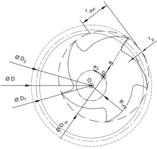
e1 e2 doc r Ø D Ø D Ø D 2 1 R mc Ø D m rp o O
Fig. 2 Parameterization of the thread milling operation
MP Definition: Dm, km RF Definition: γom, λsm Cutting plane calculation: Vi, TVi, NVi
Cutting angle calculation: γi, λs, κr
CE Calculation
Figure
Fig. 3 Mill profile (MP) - case A: P = 2 mm, Dm = 12 mm, km = 1/8
Fig. 4 Geometrical construction of the cutting edge (CE) - case A: αom= 10 °, λsm= 30 °
RF MP CE GLRF VRF2 uce lce fce P 2 Pm inf.lim. Pm sup.lim. Pm0 Pm1 Pm2 Pm3 Pm4 Pm5 Pm6 5.0 5.5 6.0 r mm 0.5 1.0 1.5 2.0 z mm km.H
Fig. 5 Cutting edge (CE) with reference planes (Pr) and normal planes (Pn) - case A: om
α = 10 °, λsm= 30 °
Fig. 6 Cutting edge (CE) with cutting planes (Pr) at point zce = P/4 - case A: αom= 10 °, sm λ = 30 ° CE Pf Ps CE(zce = P/4) Pr Pn Po CE Pr Pn CE(zce = P/4) CE(zce = P/2) CE(zce = 3P/4)
Fig. 7 Cutting edge cross sections for angle parameterization
Fig. 8 Cutting angles - case A: γom= 10 °, λsm= 30 °
-30 -20 -10 0 10 20 30 40 50 0.0 0.2 0.4 0.6 0.8 1.0 1.2 1.4 1.6 1.8 2.0 zce (mm) λλλλs γγγγn γγγγo γγγγf ( °) 0 20 40 60 80 100 120 140 160 κr ( °) gn gf go ls kr fce lce uce γn γf γo λs κr Pr∩Pi V RF Pi∩ V RF.Pi NV Pr.Pi NV i γ i γ i P RF CE.Pr TV CE TV Pr.Pn NV Pr NV λs s λ CE s P CE.Pr TV r P κr RV CE
Fig. 9 Normal rake angle (γn) for mills having an identical flute angle - λsm = 15 °
Fig. 10 Normal rake angle (γn) for mills having a constant orthogonal rake angle
γom = 10 ° -30 -20 -10 0 10 20 30 40 0.0 0.2 0.4 0.6 0.8 1.0 1.2 1.4 1.6 1.8 2.0 zce (mm) γγγγn ( °) γom = 10 ° ; λsm = 0° γom = 10 ° ; λsm = 15° γom = 10 ° ; λsm = 30° γom = 10 °, λsm = 0 ° γom = 10 °, λsm = 15 ° γom = 10 °, λsm = 30 ° fce uce lce -15 -10 -5 0 5 10 15 20 25 30 0.0 0.2 0.4 0.6 0.8 1.0 1.2 1.4 1.6 1.8 2.0 zce (mm) γγγγn ( °) γom = 0 ° ; λsm = 15° γom = 10 ° ; λsm = 15° γom = 20 ° ; λsm = 15° γom = 0 °, λsm = 15 ° γom = 10 °, λsm = 15 ° γom = 20 °, λsm = 15 ° fce lce uce