Du magnétisme frustré aux fermions fortement corrélés : approches effectives et non perturbatives

THÈSE

DOCTORAT DE L’UNIVERSITÉ DE TOULOUSE

Délivré par l'Université Toulouse III - Paul Sabatier Discipline ou spécialité : Sciences Physiques.

JURY

Claire LHUILLIER (Présidente) Benoit DOUCOT (Rapporteur) Thierry JOLICOEUR (Rapporteur)

Patrick AZARIA Michel CAFFAREL Sylvain CAPPONI

Pierre PUJOL (Directeur de Thèse) Claudio CHAMON (Codirecteur de Thèse).

Ecole doctorale : Ecole doctorale des Sciences de la Matière. Unité de recherche : Laboratoire de Physique Théorique

Directeur(s) de Thèse : Pierre PUJOL/Claudio CHAMON Présentée et soutenue par Daniel CHARRIER

Le 17 Septembre 2009

Titre : Du magnétisme frustré aux fermions fortement corrélés:

Remerciements

Cette th`ese rassemble le travail que j’ai effectu´e en trois ans dans les trois laboratoires sui-vants : le laboratoire de Physique de l’ENS Lyon, le Physics Department de Boston University et le laboratoire de Physique Th´eorique `a Toulouse. Cette ”d´elocalisation” m’a permis de mul-tiplier les exp´eriences tant professionnelles que personnelles au cours de mes trois ann´ees de th`ese. Dans chaque laboratoire, j’ai pu cˆotoyer des chercheurs passionn´es, ainsi que des jeunes doctorants et post-docs venant de tous les horizons. Cette th`ese est un peu le produit de ces rencontres. Je tiens donc `a remercier particuli`erement :

– Pierre Pujol, bien sˆur, pour m’avoir laiss´e l’opportunit´e d’entreprendre ce parcours ori-ginal et formateur. Grˆace `a Pierre, j’ai dispos´e d’une grande libert´e de choix dans mes sujets et dans le d´eroulement de ce projet. J’ai pu mener `a bien mon s´ejour `a Boston et mon transfert `a Toulouse. Il m’a mis le pied `a l’´etrier dans le monde de la recherche. – Claudio Chamon, for having welcomed me in Boston... although he knew nothing about

me ! I still remember the first time we met, when I was supposed to work on string-nets condensations. Finally, we ended up with this project and a new word in English vocabu-lary. I hope we will find the opportunity to work together again, on our groundstatability issue or on something else.

– Fabien Alet, pour son soutien constant dans les moments difficiles. Pour m’avoir appris `a faire de vrais simulations. Pour ne pas s’ˆetre ´enerv´e quand j’ai demand´e pour la 10i`eme fois pourquoi ALPS ne voulait pas compiler.

– Sylvain Capponi, pour sa gentillesse, pour l’int´erˆet qu’il a port´e `a mon travail et son implication dans mes projets.

– Mon jury de th`ese, et en particulier les rapporteurs, pour avoir lu une premi`ere version du manuscrit parsem´ee de fautes et de coquilles ; Claire Lhuillier pour sa gentillesse et pour avoir accept´e d’ˆetre pr´esidente de mon jury, Benoit Dou¸cot, Thierry Jolicoeur et Patrick Azaria pour tous leurs commentaires constructifs, et Michel Caffarel.

– Les autres chercheurs qui m’ont aid´e par leurs suggestions et leurs r´eponses, en particu-lier : Fran¸cois Delduc, Peter Holdsworth, Dider Poilblanc, Rapha¨el Chetrite et Cl´ement Sire.

– La multitude de doctorants et post-docs que j’ai rencontr´ee au cours de ces trois ans et en particulier : Rapha¨el Chetrite, Patrick Loiseau, Nicolas Mallick et Michel Tsamados

– Ma famille qui a dˆu supporter les multiples d´em´enagements ainsi que la distance et l’´eloignement.

Table des mati`

eres

1 Frustrated Magnetism in d > 1 and effective approaches 6

1.1 From quantum magnets to dimer models . . . 7

1.1.1 Frustrated quantum magnets . . . 7

1.1.2 Non magnetic states . . . 11

1.1.3 Quantum Dimer models . . . 14

1.2 Unconventional phase transitions in dimer models . . . 18

1.2.1 From the QDM to interacting classical dimer models . . . 19

1.2.2 The interacting classical dimer model on the cubic lattice . . . 21

1.2.3 Emerging scenarios for generic unconventional phase transitions . . . 25

1.3 Simulation of a lattice gauge model. . . 37

1.3.1 Simulation techniques . . . 38

1.3.2 The flowgram method . . . 44

1.3.3 Results . . . 48

1.3.4 Generalized interacting dimer model on the cubic lattice . . . 53

2 Groundstatability of fermionic wavefunctions. 57 2.1 Defining groundstatability . . . 58

2.1.1 The stochastic matrix approach . . . 58

2.1.2 The groundstatability problem . . . 65

2.1.3 Groundstatability in many-body physics . . . 66

2.2 Fermionic wavefunctions . . . 71

2.2.1 From the Hubbard model . . . 72

2.2.2 Mean Field Solutions . . . 74

2.2.3 Other Fermionic wavefunctions of interest . . . 77

2.3 Numerical procedure . . . 81

2.3.1 Inverse Monte Carlo Method . . . 81

2.4 Fermionic Hamiltonians of groundstatable wavefunctions. . . 87

2.4.1 Fermions in 1D. . . 87

2.4.2 Fermions in 2D . . . 91

2.4.3 Conclusion . . . 103

3 Study of an anisotropic spin tube with integer spin. 105 3.1 Strong coupling approach : J_! << J_⊥. . . 107

3.1.1 Classical equilibrium configurations . . . 107

3.1.2 Ground state of the quantum triangle. . . 108

3.2.1 The Heisenberg integer chain. . . 110

3.2.2 The quantum spin tube . . . 113

3.2.3 The special case of S = 1 . . . 114

3.3 Large S approach . . . 117

3.3.1 Linear spin-wave theory . . . 118

3.3.2 Low energy degrees of freedom . . . 122

3.3.3 Non Linear σ model . . . 123

Introduction

Cette th`ese est consacr´ee `a l’´etude de th´ematiques apparues r´ecemment en Mati`ere Condens´ee th´eorique. Elle aborde des sujets divers, comme le magn´etisme quantique frustr´e en une et deux dimensions, les mod`eles de dim`eres classiques, et les probl`emes de fermions en interac-tion. Le domaine de la Mati`ere Condens´ee est vaste, tant dans la vari´et´e des probl´ematiques pos´ees que dans les m´ethodes pour les r´esoudre. Avec le perfectionnement constant des tech-niques exp´erimentales, apparaissent sans cesse de nouvelles r´eponses mais aussi de nouveaux probl`emes. A ce titre, on peut citer le renouvellement permanent des id´ees autour de l’effet Hall quantique depuis 1982 (d´ej`a deux prix Nobel !), le myst`ere toujours non r´esolu de la supracon-ductivit´e `a haute temp´erature critique dans les oxydes de cuivre, les d´eveloppements th´eoriques et exp´erimentaux sur le graph`ene, l’apparition de nouveaux supraconducteurs `a base de fer... Le d´eveloppement des simulations num´eriques a parachev´e la transformation de la physique de la Mati`ere Condens´ee. La d´etermination quasi-syst´ematique des propri´et´es d’un mod`ele `a l’aide de simulations a permis l’´etude de syst`emes plus complexes, o`u les fortes corr´elations entre particules rendent inop´erantes les approches traditionnelles. De nouvelles phases de la mati`ere ont ainsi ´et´e d´ecouvertes : glace de spins, supersolide, phases n´ematiques, liquide de spin... Enfin, la Mati`ere Condens´ee th´eorique se situe au point de croisement entre la physique statistique et la m´ecanique quantique. Elle est donc parfaitement adapt´ee au cadre de la th´eorie quantique des champs et `a ses m´ethodes, notamment le groupe de renormalisation et la th´eorie des groupes.

Cette th`ese est divis´ee en trois parties, chacune traitant d’un sujet diff´erent. La premi`ere traite des approches effectives du magn´etisme quantique frustr´e en deux dimensions, la deuxi`eme des probl`emes de fermions en interaction et la troisi`eme du magn´etisme quantique en une dimension. Nous nous sommes tout d’abord int´eress´es `a mieux comprendre la physique non conventionnelle de certains mod`eles effectifs utilis´es pour d´ecrire le magn´etisme quantique dans la mati`ere : les mod`eles de dim`eres. En particulier, le mod`ele de dim`eres sur r´eseau cubique pr´esente une tran-sition de phase du second ordre entre un ordre colonnaire `a basse temp´erature et une phase critique `a haute temp´erature o`u les corr´elations dim`eres-dim`eres d´ecroissent alg´ebriquement. Le caract`ere tr`es diff´erent de ces deux phases et la possibilit´e d’une transition continue entre les deux en font un exemple typique de transition de phase ”exotique”. L’existence de ce type de transition est encore aujourd’hui sujette `a controverse. En effet, contrairement `a la th´eorie usuelle des transitions de phase, ces transitions ne peuvent s’expliquer dans le cadre de la bri-sure spontan´ee de sym´etrie d’un param`etre d’ordre. Dans le cas du mod`ele de dim`eres, nous avons pu d´emontrer `a l’aide d’arguments de dualit´e que la transition entre la phase dipolaire et la phase ordonn´ee peut ˆetre comprise par le m´ecanisme de Higgs. La simulation du mod`ele de jauge sur r´eseau correspondant a permis de confirmer l’existence d’une classe g´en´erique de transitions exotiques.

toute simulation Monte Carlo pour des syst`emes de fermions sur r´eseau. Ici, nous cherchons `a savoir si, en fixant l’´energie cin´etique d’un Hamiltonien de fermions, une fonction d’onde donn´ee peut ˆetre l’´etat fondamental du syst`eme, pour un choix appropri´e de l’´energie potentielle. Il est en effet beaucoup plus ais´e de fixer la forme de l’´energie cin´etique `a l’aide des principes g´en´eraux de sym´etries que celle de la fonction d’onde. Cette ´etude a montr´e que certaines fonc-tions d’onde ne pouvaient jamais ˆetre le fondamental d’un syst`eme physique alors que d’autres le pouvaient. On dit alors que la fonction d’onde est fondamentalisable (groundstatable en an-glais, l’invention de ce mot est due au Prof. Claudio Chamon). Son application `a diverses fonctions d’onde supraconductrices ou magn´etiques a permis l’obtention d’une vari´et´e d’Hamil-toniens fermioniques dont l’´etat fondamental et les propri´et´es sont connus avec pr´ecision. En particulier, il a ´et´e possible d’obtenir des Hamiltoniens o`u ordre magn´etique et supraconducti-vit´e sont simultan´ement favoris´es.

Dans un troisi`eme temps, nous nous sommes attach´es `a d´ecrire des probl`emes de chaˆınes de spins frustr´ees `a l’aide d’un mod`ele sigma non lin´eaire. Il est bien connu que les chaˆınes de spins pr´esentent un comportement tr`es diff´erent selon que le spin soit entier ou demi-entier : dans le premier cas, les corr´elations spin-spin d´ecroissent alg´ebriquement avec la distance alors que pour les chaˆınes de spin entier, les corr´elations sont de courte port´ee. Une approche sigma non lin´eaire fait apparaˆıtre la distinction entre les deux cas, avec l’apparition d’un terme ”to-pologique” dans l’action uniquement pour les spins demi-entier. Ici, nous nous int´eressons `a un mod`ele de tube de spin o`u des triangles de spins sont coupl´es antiferromagn´etiquement. La description continue du mod`ele fait intervenir un param`etre d’ordre appartenant `a SO(3). Nous discutons de cette approche dans le cas o`u les couplages entre spins ne sont pas tous identiques. En particulier, nous analysons l’importance des d´efauts topologiques qui conduisent `a une physique radicalement diff´erente dans le cas isotrope et anisotrope. La possibilit´e de nou-veaux points critiques dans le diagramme du tube de spin est soulev´ee.

La premi`ere et la seconde section contiennent d’importants travaux num´eriques en plus des r´esultats analytiques. Bien que les sections soient bien d´elimit´ees, on trouvera de nombreuses passerelles entre les diff´erents sujets trait´es.

Chapitre 1

Frustrated Magnetism in d > 1 and

effective approaches

Dans cette premi`ere partie, nous allons nous familiariser avec la physique du magn´etisme frustr´e. L’´etude du magn´etisme forme une branche sp´ecifique du probl`eme `a N corps. En phy-sique th´eorique, son analyse repose essentiellement sur des mod`eles de ”spins” en interaction. Diff´erentes ”sortes” de spins ont ´et´e invent´es pour d´ecrire la mati`ere. Certains sont de simples fl`eches s’orientant comme l’aiguille d’une boussole. D’autres sont des op´erateurs, assujettis `a une certaine alg`ebre, et agissant dans l’espace de Hilbert des ´etats. Dans le premier cas, on parlera de magn´etisme classique, et on se r´ef`erera au deuxi`eme cas comme celui du magn´etisme quantique. Il existe de nombreux ponts entre les deux familles de mod`eles. Souvent, lorsqu’un probl`eme quantique est trop compliqu´e `a r´esoudre, on tente de se ramener `a un mod`ele clas-sique associ´e : on dit qu’on se place dans une ”approximation semi-clasclas-sique”. Mais il existe aussi des cas o`u cette approche n’est pas valable. Cela arrive quand le syst`eme quantique est ”frustr´e”. Dans ce cas, les propri´et´es du mod`ele, et notamment celles de l’´etat fondamental, sont d´etermin´ees par des effets purement quantiques. Des phases nouvelles, aux caract´eristiques exotiques, peuvent apparaˆıtre. La nature des transitions entre ces phases est, elle-aussi, inha-bituelle.

Certaines de ces phases quantiques ont soulev´e un profond int´erˆet : ce sont les phases de dim`eres. Une ”physique des dim`eres” est ainsi apparue peu `a peu. C’est dans ce cadre que nous avons effectu´e nos premiers travaux. En particulier, nous nous sommes attach´es `a comprendre cer-taines transitions de phase non conventionnelles dans ces syst`emes.

Le d´eroulement de cette premi`ere partie se pr´esente comme suit : tout d’abord, nous intro-duisons la notion de magn´etisme frustr´e en m´ecanique quantique sur l’exemple du mod`ele de Heisenberg. Puis, nous d´ecrivons comment les mod`eles de dim`eres peuvent fournir une ap-proche effective pour la compr´ehension du magn´etisme frustr´e. Enfin, nous nous focalisons sur le cas d’un mod`ele particulier : le mod`ele de dim`eres en interaction sur r´eseau cubique. Ce syst`eme pr´esente une transition de phase particuli`ere. Nous proposons une explication pour cette transition en coh´erence avec d’autres th´eories apparues r´ecemment dans la litt´erature. Nos assomptions sont appuy´ees par des simulations Monte Carlo.

1.1

From quantum magnets to dimer models

Nous d´ebutons avec un bestiaire non exhaustif des diff´erentes phases de la mati`ere ren-contr´ees en magn´etisme frustr´e. Celles-ci se divisent grossi`erement en deux cat´egories : les phases ordonn´ees de type N´eel et les phases quantiques non ordonn´ees magn´etiquement (nous ne parlerons pas ici des phases n´ematiques). Apr`es avoir d´ecrit les propri´et´es des diff´erentes phases de dim`eres, nous nous tournons vers l’Hamiltonien de Rokhsar-Kivelson (RK), adapt´e `a la mod´elisation de ces phases. Cet Hamiltonien a un diagramme de phase riche et un point critique particulier : le point RK. Ce point nous permet de faire le lien entre les ´etats de dim`eres quantiques et les mod`eles de dim`eres classiques que nous allons ´etudier par la suite.

1.1.1

Frustrated quantum magnets

In this section, we will mainly be interested in the quantum Heisenberg model with antifer-romagnetic couplings : ˆ H = J ! <ij> ˆ Si· ˆSj, (1.1)

where the sum is restrained to nearest neighbor interactions and J > 0. In this chapter, we will essentially focus on spin-1/2 operators satisfying the well-known SU (2) Lie algebra :

[Sα, Sβ] = i"αβγSγ. (1.2)

The analytic solution of this model is not known. On the other hand, the related classical problem, where spin operators are replaced by standard vectors, is easier to address. That is why, by looking at the possible solutions of (1.1), a good starting point is to look for a semi-classical picture of the ground state, where quantum effects are added perturbatively into the classical solution.

The semi-classical picture : the N´eel state

The Ferromagnet Let’s first consider the case when J < 0. For spins 1/2, a ground state of the Hamiltonian is the fully polarized ferromagnetic state :

|ˆz! ="

i

|i, +!, (1.3)

where _{|i, +! is the single spin state with : S}z

i|i, +! = 12|i, +!. Other possible ground states can be obtained by the application of the rotation operators :

|ˆu! = eiStotz φeiStoty θ"

i

|i, +!, (1.4)

where Stot is the total spin and (θ,φ ) are the Euler angles of the unit vector u. These states

have a non-zero magnetization per site m ="Si! = 1₂u and they break the global SU (2)

sym-metry of the Hamiltonian. These states are the quantum version of the classical configurations which minimize the classical energy of the system. Thus, for the ferromagnet, the classical and quantum problems are in direct correspondence.

1.1. FROM QUANTUM MAGNETS TO DIMER MODELS

Coordination 2 < Si.Sj >

Lattices number per bond M/Mcl

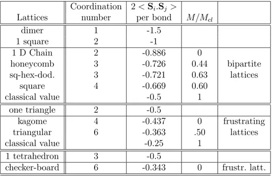
dimer 1 -1.5 1 square 2 -1 1 D Chain 2 -0.886 0 honeycomb 3 -0.726 0.44 bipartite sq-hex-dod. 3 -0.721 0.63 lattices square 4 -0.669 0.60 classical value -0.5 1 one triangle 2 -0.5 kagome 4 -0.437 0 frustrating triangular 6 -0.363 .50 lattices classical value -0.25 1 1 tetrahedron 3 -0.5

checker-board 6 -0.343 0 frustr. latt.

Tab. 1.1 – Quantum energy per bond and sublattice magnetization in the ground state of the spin-1/2 Heisenberg Hamiltonian on various simple cells and lattices. The sq-hex-dod. is a bipartite lattice formed with squares, hexagons and dodecagons. See [1] for references.

The Antiferromagnet Repeating the same argument for the case J > 0, a simple proposal for the antiferromagnetic (AF) ground state on a square lattice would be :

|ΨAF0 ! = "

i∈A,j∈B

|i, +!|j, −!, (1.5)

where A and B denotes the two sublattices. However, this state is not an eigenstate of (1.1). The semi-classical N´eel state, if it exists, emerges from the dressing of the state (1.5) by the quantum fluctuations produced by ˆH. The main assumption here is that these quantum corrections won’t

qualitatively change the classical picture but only renormalize the properties of the system, that is, the ground state energy and its magnetization. Here are the main properties of the N´eel state : – It has a non zero magnetization per site m_{$= 0 whose value is smaller than the classical} magnetization given by state (1.5). The rescaling of the classical value depends on the geometry of the lattice (see table 1.1). It breaks the SU (2) symmetry of the Hamiltonian in the thermodynamic limit.

– Correspondingly, it has long-range spin-spin correlation functions.

– The ground state energy is renormalized by the zero-point energy of the quantum fluc-tuations.

– It admits excitations in its spectrum, the magnons or ”spin-waves”. These carry a∆ S = 1 excitation. Contrary to an Ising-like state such as (1.5), these excitations are gapless. These characteristics can be obtained in a simple perturbative way : the linear spin-wave theory. We shall see an application of this theory in Chapter 3. The linear spin-wave theory tells us that the standard excitations are oscillators-like, characterized by a dispersion law ωk. The gapless excitations are due to the existence of soft points in the Brillouin zone, where ωk = 0, and around which the dispersion law becomes linear. In particular, the order parameter is

reduced by a factor : m_{% 1 −} 1 N ! k∈BZ # 1 ωk − 1 $ . (1.6)

Thus, the renormalization of the order parameter is dominated by the fluctuations in the low energy modes. Since ω(k) _{∝ k around this point, it is straightforward to show that the sum} in (1.6) will be well defined only in dimension two or higher. In one dimension, the sum di-verges, which is a first example of the breakdown of the perturbative semi-classical approach. In fact, this last point can be related to a well-known result in condensed matter theory : the Mermin Wagner theorem [2]. This states that no spontaneous breaking of a continuous symmetry can occur in one dimension. In 1d, the quantum fluctuations will always be strong enough to restore a continuous symmetry. The same theorem applies in two dimensions at non-zero temperature because of the thermal fluctuations. Accordingly, we can picture the landscape of quantum magnets following the semi-classical approach :

– in 1d, the system is always disordered.

– in 2d, the system is magnetically ordered at T = 0 and disordered otherwise.

– in 3d, the system undergoes a phase transition at a finite temperature between an ordered state and a disordered state.

δ O β γ α 2 U 1 U

Fig. 1.1 – Left : the checkerboard lattice. Right : The Kagome lattice.

Most of these conclusions drawn from the spin-wave analysis are sufficient for many systems. However, the existence of the semi-classical picture is in no way guaranteed. Indeed, strong quantum fluctuations can destroy the classical order. First, as we just saw, the perturbative approach is unfit to describe any 1d system like spin chains and magnetic ladders. The physics of 1d systems is rich with many unusual effects due to the reduced dimensionality. The 1d case will be reviewed in detail in chapter 3. Second, looking at Table 1.1, we see that for some special geometries of the lattice in 2d , like the kagome lattice (Figure 1.1 left) and the checkerboard lattice (Figure 1.1 right), the magnetization vanishes even at T = 0 in contradiction with the perturbative scenario [3, 4]. Both are examples of ”pure” quantum phases of matter, in the

1.1. FROM QUANTUM MAGNETS TO DIMER MODELS

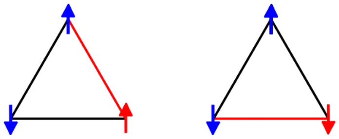
Fig. 1.2 – A simple example of frustrated magnet : Ising spins on a triangle. Red links denote frustrated bonds.

sense that they have no classical counterpart. Non perturbative approaches are necessary to describe such a state. Note also that these are frustrated lattices. That is why, to understand the breakdown of the N´eel order, we need to introduce the notion of frustration.

Frustration

The paradigm of the frustrated spin system is certainly the classical Ising model on the triangular lattice. Imagine to put three Ising spins (i.e up/down arrows) on the corners of a triangle (see Figure 1.2). The spins interact antiferromagnetically and tend to anti-align. Two configurations have then the same energy. The system is said to be ”frustrated” because it can-not minimize its energy on all the bonds. On a triangular lattice, this ”degeneracy” will extend to many configurations differing by local moves. Hence, the magnetization will be weakened by the frustrating bonds. At a quantum level, the same mechanism holds for the ground state properties. The frustration on the bonds enhances the quantum fluctuations around the ground state, which brings down the magnetization. The Ising model on the triangular lattice provides a first example of what is referred to as geometric frustration.

There is yet another possibility to frustrate the system : it is by adding competing interac-tions. Consider for example the J1 _{− J}2 model on the triangular lattice :

ˆ H = J1 ! <ij> ˆ Si· ˆSj + J2 ! <<ik>> ˆ Si· ˆSk, (1.7)

where we have included second nearest neighbor antiferromagnetic couplings. These additional couplings clearly oppose the nearest neighbor interactions and if strong enough, they can lead to a different ground state from the original N´eel state. In fact, for 1/8 < J2 < 1, the competing

interactions lead to a continuous degeneracy of the ground state at the classical level. This degeneracy is partially lifted by the effects of the spin-waves (the mechanism of selection of the ground state for is actually not as simple as it looks. It involves the process of ”order by disorder”, see below). On the square lattice, when J2 _{∼ 0.5J}1, the ground state displays no magnetization at all, and is totally unconventional in the sense of the semi-classical picture. Failure of the adiabatic continuation If the frustration is strong enough, the magnetiza-tion will be reduced to zero, even at T = 0. That is why frustramagnetiza-tion is the essential ingredient for the apparition of non-N´eel states in quantum magnets in 2d. The kagome lattice, the che-ckerboard lattice or the pyrochlore lattice in 3d (lattice of corner sharing tetrahedra) are all highly frustrating. On contrast, simple bipartite lattices are very weakly frustrated and often

develop a N´eel order. The effect of frustration can be twofold. On one hand, it can select a par-ticular magnetic order between various ground states by the mechanism of ”order by disorder”. In this case, a given state has a larger density of low lying excitations which implies a smaller zero point energy. This state is thus energetically ”favored” by the quantum fluctuations [5]. This is what happens for the J1_{− J}2 models [6]. On the other hand, it can have more drastic effects. The ground state can become totally non-magnetic, the spin-spin correlations decay exponentially to zero and the spin excitations change in nature and become gapped. This is this last situation that we will focus on for now.

1.1.2

Non magnetic states

While the existence of non magnetic states in one dimensional systems was a well-known fact, the possibility of having a state without magnetic order in d > 1 at T = 0 has been debated at length. For example, the Heisenberg model on the non bipartite triangular lattice has been a long-standing candidate for being non-magnetic but it was finally found to have a small but non zero N´eel order [7]. Finally, the first example of a truly non-magnetic state at

T = 0 was discovered by Shastry and Sutherland in 1981 [8]. Since then, many models have

been found to behave differently from the classical picture.

The Quantum paramagnet The simplest example of a singlet state that one can think of is the quantum paramagnet, where spin variables are essentially free. It is a disordered phase with no order and where spin-spin correlations decay fastly. It is the unique ground state of the Heisenberg Hamiltonian (1.1) at T $= 0 in 2d, and above the critical temperature in 3d.

All spin excitations are gapped. As we will see in Chapter 3, the 1d problem at T = 0 is more subtle. The quantum paramagnet state is rather trivial and not really in contradiction with the semi-classical picture of above.

Valence Bond States If the couplings between the spins become very strong, we expect that a spin-wave description of the theory should not work very well. On the contrary, one can think of describing the ground state in terms of pairs of spins forming S = 0 singlet states over short distances [9]. Such a pair can be written as :

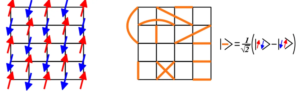
|(ij)! = √1

2(| ↑i↓j! − |↓i↑j!) . (1.8)

States formed from such a superposition of singlets over the lattice are called Valence Bond (VB) states (see Fig 1.3). Different kinds of VB states have been proposed to describe the low-energy physics of frustrated magnets and beyond that, the physics of related materials such as the high-Tc superconductors [10]. Models exist with long range [11] and short range [12] versions of Valence Bonds. Here, we will concentrate on the latter case and essentially detail two particular classes of short range VB states. These are :

– the Valence Bond Crystals.

– the Resonating Valence Bond states (also referred to as Spin Liquids). Valence Bond Crystals

In some situations, the ground state of (1.1) is accurately described by a simple product of singlet objects. For instance, the ground state of the Heisenberg model on the checkerboard

1.1. FROM QUANTUM MAGNETS TO DIMER MODELS

Fig. 1.3 – Left : Classical picture of the N´eel state. Right : Quantum valence bond state.

lattice is a product of plaquettes [4] :

|V BC! = "

∗

|α, β, γ,δ ! (1.9)

|α, β, γ,δ ! = |α,δ !|γ,β ! + |α,β !|γ,δ !.

where|α,β ! is a singlet. Such a phase does not show any magnetic long-range order. However,

it develops an order in the plaquettes as observed with exact diagonalization techniques. This kind of phase is dubbed as a Valence Bond Crystal (VBC). VBC states are pure S = 0 states and are identified by the following characteristics :

– The ground state is a superposition of a small number of singlet configurations. – there exists long-range dimer-dimer or plaquette-plaquette correlations.

– the singlet order breaks some symmetries of the lattice in the thermodynamic limit. – Spin-spin correlations are short-range.

– There exists only gapped spin excitations.

Fig. 1.4 – The two VBC ground states on the checkerboard lattice.

Realizations of VBC include the J1−J2 model on the hexagonal lattice [13] and presumably on the square lattice close to the point of maximum frustration J2 ∼ 0.5J1 [5]. Exact diago-nalization methods show also that dimer phases exist in the J_{− K model with ring-exchange} interactions [14]. Large-N limits of the Heisenberg model (where the SU (2) Lie algebra of the

spin is extended to SU (N )) also provide several examples of Valence Bond Crystals [15, 16]. Significantly, no examples of VBC phases with pure spin-1

2 models on non bipartite lattice have been found so far. It seems that bipartiteness is an essential ingredient for the stability of a VBC phase.

An important distinction between the different VBC phases are the explicit VBC and the

spontaneous VBC. In the latter case, such as in the checkerboard lattice, the phase breaks

spontaneously the symmetries of the lattice in the thermodynamic limit. This therefore leads to a degeneracy of the ground state. On the contrary, explicit VBC like the Shastry-Sutherland model display a dimer order but do not break any additional symmetry since the Hamiltonian is already non-symmetric. Experimentally, CaV4O9 is the first Heisenberg-like system where the magnetic excitations were found to be gapped [17]. It can be represented by a Hamiltonian with nearest neighbor and next nearest neighbor antiferromagnetic couplings on a depleted square lattice where one site out of five is missing. Another example is the SrCu2(BO3)2 which is a good realization of the Shastry-Sutherland model [18]. In both cases, we have explicit VBC. Resonating Valence Bond states

On the opposite of the VBC, one could think of a frustrated system which allows many different singlet configurations to be present in the ground state. Indeed, the off-diagonal part of the Heisenberg Hamiltonian acts like a kinetic energy for the singlets and connects almost any pair of dimer coverings. If the weights of the configurations were properly picked up in the ground state, one could imagine that such a phase would be stabilized by resonances. This idea of a Resonating Valence Bond state was first suggested by Anderson [9] by analogy with Pauling’s idea of resonance in organic cycles. A RVB wavefunction reads :

|RV B! =!

C

AC|C!, (1.10)

where _{|C! is a singlet configuration. Depending on the weights AC}, long-range or only short-range Valence Bonds can be allowed in the RVB wavefunction. In the first case, the system can develop a magnetic long-range order [11]. In the latter, all the correlations are short-ranged (spin liquid). The characteristics of a short-range RVB are :

– the ground state is a superposition of an exponential number of singlet configurations. – there is nor magnetic order neither singlet order (all the correlation functions are

short-range).

– it does not break any symmetry in the thermodynamic limit. – the excitations are gapped.

– the ground state exhibits a subtle topological degeneracy.

If not for the last point, we wouldn’t be able to distinguish the spin liquid from the quantum paramagnet. As we will see, due to its topological properties, the spin liquid presents additional features among which the possibility of carrying non-trivial excitations, the spinons. It can be seen as a cooperative paramagnet : the energy scale of the interactions exceeds that set by the temperature, and nonetheless no long-range order ensues. Unfortunately, all efforts to find a realization of a spin liquid in a Heisenberg model has proven delusive so far. But the search for the short range RVB latter led to the expansion of a new class of models, the quantum dimer models.

1.1. FROM QUANTUM MAGNETS TO DIMER MODELS

Fig. 1.5 – Separating a triplet in a VBC phase destabilizes the crystalline order. A ”string” tension tends to bring the two spinons back together. By contrast, it is possible to move the spinons in a RVB by a local rearrangement of the dimers.

Deconfinement of spinons Heuristically, the RVB state can be seen as a soup of disordered dimers. The elementary excitations of both VBC and RVB states are S = 1 triplets created by the breaking of a dimer. This excited triplet can be seen as a pair of spin-1

2 particles called

spinons. The deconfinement of the spinons are one of the most striking feature of a spin liquid.

In a crystal of dimer, separating two spinons will cost an energy increasing with the distance between them since this separation means disordering more and more the aligned dimers (see figure 1.5). On comparison, it won’t cost any additional energy to disjoin the two spinons in a RVB since the dimers are already disordered. A similar mechanism involving holes and spinons appears when the quantum dimer model is doped [19].

1.1.3

Quantum Dimer models

In 1988, Rokhsar and Kivelson [12] speculated their famous quantum hard core dimer model (QDM) on the square lattice. Their original intention was to describe a system of interacting Cooper pairs. But with no hallmarks of a spin liquid in the Heisenberg model, the QDM eventually brought an entire set of new models for the search of unconventional phases of matter. One of the greatest achievements of the QDM was the discovery of a real spin liquid on the triangular lattice by Moessner and Sondhi [20]. Here, we will mainly focus on the QDM on bipartite lattices.

Hilbert space

The underlying hypothesis behind the QDM is that the different singlet phases in spin systems, VBC and short-ranged RVB, are gapped. If the spin gap is large enough, it will need a lot of energy to break a singlet into a triplet and one can assume that the low-lying excitations

are just rearrangements of the singlet structure. Accordingly, the manifold of low energy states would be correctly spanned by the set of short-range valence bond coverings. Thus, the QDM reduce a problem of interacting spins into a problem of interacting dimers. In a QDM, the elementary degree of freedom is a dimer. The Hilbert space is defined by enforcing a hard constraint on the sites of the lattice. This constraint consists of demanding that each site forms a dimer with one, and only one, of its nearest neighbors. Therefore, the configurations included in the dimer Hilbert space are the set of nearest-neighbor dimer coverings of the lattice 1_. Because of the hard-core constraint, the number of allowed configurations is much smaller than in a spin model on the same lattice. For a square lattice with N sites, the Hilbert space of the latter has a dimension 2N _{while the number of ways to cover the lattice with dimers}

grows asymptotically as (1.3385...)N _{[21, 22]. It is important to stress out that dimers are}

not independent degrees of freedom as spins are. If one tries to displace one dimer, the move must be accompanied by a local rearrangement of the dimer configuration, as permitted by the constraint.

The Rokhsar Kivelson model

The Rokhsar-Kivelson Hamiltonian is defined by : ˆ

HRK =

! Plaquettes

[_{−t (|!}! _!!_{! "!}! !_{!| + |!}! _!!_{! "!}! _!!_{|) + V (|!}! _!!_{! "!}! _!!_{| + |!}! _!!_{! "!}! _!!_{|)] .} (1.11)

The first term is a kinetic term, which flips two parallel dimers on a plaquette. The second term is a potential energy proportional to the number of parallel dimers in a given configuration. Interactions between plaquettes can be either attractive V < 0 or repulsive V > 0. Depending on the relative sign of V and t, parallel dimers will be favored or penalized.

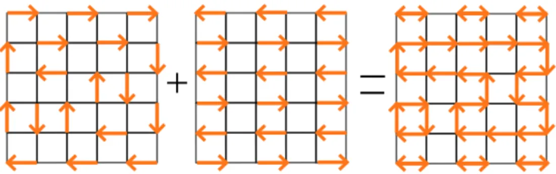
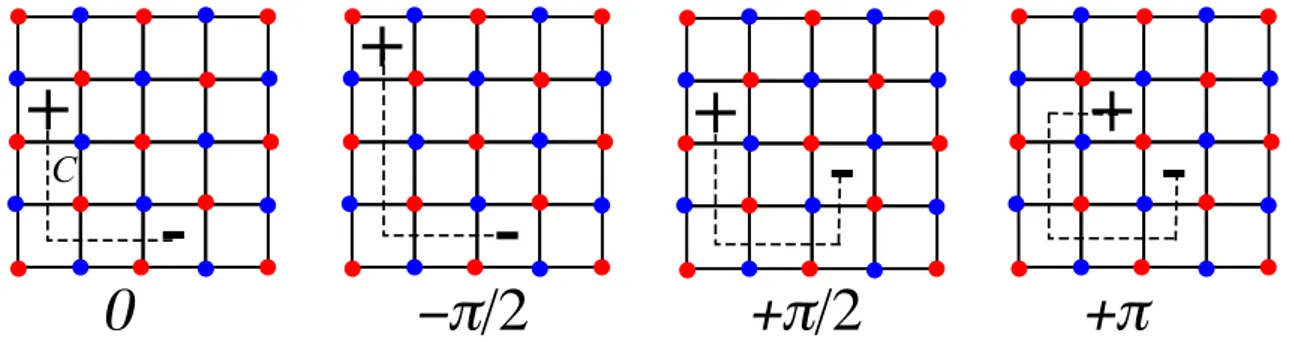
Topological properties The RK model gives us the first occasion to discuss the importance of topology when dealing with statistical models on non-trivial geometries. The peculiar proper-ties of the RK model appear when we impose periodic boundary conditions in the two directions and lay down the lattice on a torus. As shown by Rokhsar and Kivelson, dimer configurations on the torus can be labelled by winding numbers. To determine the winding numbers of a dimer configuration_{C, one can consider one of the columnar configurations C}0 as a reference configu-ration and superpose_{C and C}0 on a single graph (see Figure 1.6). Dimers inC are oriented from one sublattice to the other, and inversely forC0. The transition graph betweenC and C0appears as a graph of oriented loops. The winding numbers count how many loops encircle the torus in the two directions. The point is that these loops are non-contractible under the Hamiltonian dynamics (1.11). Indeed, the Hamiltonian (1.11) does not connect configurations with different winding numbers. In other words, the Hilbert space is divided in separated sectors which ”do not talk to each other”. In the language of topology, these sectors correspond to the different classes of the fundamental homotopy group of the torus given by :

Π1(torus) =Z × Z, (1.12)

hence the name topological sectors, each sector being associated with a pair of integers.

1_{Note that in the spin Hilbert space, the set of nearest neighbor Valence Bond configurations forms a}

linearly independent family of vectors but it is not orthogonal. In the dimers Hilbert space, this family has been orthogonalized.

1.1. FROM QUANTUM MAGNETS TO DIMER MODELS

Fig. 1.6 – Left : a given (oriented) configuration of dimers. Middle : The reference configuration we choose, Right : the transition graph made of closed loops. Loops are oriented to take care of the bipartiteness of the lattice.

Note that the geometry of the lattice matters a lot when dealing with the topological division of the space. Non-bipartite lattice, such as the triangular lattice, can have only non-oriented graphs. This reduces the number of topological sectors to only four possibilities.

Perron-Frobenius theorem The Rokhsar Kivelson system holds another important pro-perty. For V _{≥ t ≥ 0, all the off-diagonal elements of (1.11) are negative and the diagonal} elements are positive. An important result of linear algebra, the Perron Frobenius theorem, tells us then that the ground state of the system has zero energy, is unique (up to the topolo-gical degeneracy discussed above), nodeless and has positive weights [23]. We will come back to this theorem when discussing about fermions in Chapter 2.

Phase diagram Fixing t ≥ 0 and varying V from large positive values, we encounter the

subsequent phases :

– For 0 < t < V , staggered configurations with no flippable plaquettes are zero-energy eigenstates of (1.11). Since the Hamiltonian is semi-definite positive in this case (with a minimal energy per plaquette V _{− t > 0), or equivalently due to the Perron Frobenius} theorem, the staggered configurations are the (topologically degenerated) ground states. On the square lattice, there are exponentially many such states. All other topological sectors are higher in energy.

– For 0 < V < t : Quantum Monte Carlo computations show that the ground state is in a plaquette phase down to 0.6t < V [24]. This phase should be interpreted in a mean field sense : ordered plaquettes indicate the positions where the dimers have a larger probability to sit. On such a position, a pair of parallel dimers constantly flips between the horizontal and vertical configurations. This state does break the translational symmetry but conserve the rotation symmetry.

– For V < 0, the system seeks to maximize the number of flippable plaquettes. The four columnar configurations are energetically favored. The ground state breaks all the lat-tice symmetries. Recent exact diagonalization results tend to indicate that there exists a mixed phase between the columnar and the plaquette phase for 0 < V < 0.6t [25].

RK !"#$$%&%' !"#$$%&%' ()!*+"%*,-./. 012-34#& 012-34#& 567 8+9-+' :2#9-%""% ;+<%' V/J

"&

+#4$-2#&

*9-#&%

Fig. 1.7 – Phase diagram of the quantum dimer model on the square and triangular lattice. Contrary to the square lattice, the triangular lattice displays a whole RVB phase below the RK point characterized by a gap to all excitations and short-range correlations for any local observable [25].

To sum up, the QDM on the square lattice features three examples of VBC phases, one colum-nar, one plaquette and one staggered, but there is no spin liquid phase.

Rokhsar-Kivelson point In addition, the model admits a particular critical point at V = t where the ground state is given by the exact superposition of all dimer coverings :

|Ψ0! = 1 √ Z ! C |C!. (1.13)

This can be seen from the fact that the RK Hamiltonian can be rewritten as a sum of positive projectors : ˆ HRK = V ! C,C! [_{|C!"C| + |C}%_!"C%_{| − |C!"C}%_{| −|C} %_{!"C|] ,} (1.14) where_{C and C}% _{are two dimer configurations differing by the flip of two parallel dimers. Indeed,}

one can check that the state (1.13) is annihilated by each of the projectors in (1.14). The RK point shares many properties of the RVB spin liquid. In fact :

– The ground state wavefunction is the sum of all dimer coverings. It supports resonances between different dimer configurations.

– The ground state exhibits a topological degeneracy. The sum of all configurations in each topological sector is in fact a ground state. In particular, the different staggered configurations remain zero-energy eigenstates at V = t as the unique member of their topological sector.

– If one allows for monomers (i.e sites not linked to a dimer), there are deconfined at the RK point.

The RK point exhibits a particular behavior : topological order. Topological order describes the situation in which the ground states of the different topological sectors are exactly dege-nerate. It is like conventional order where the spontaneous breaking of a symmetry leads to

1.2. UNCONVENTIONAL PHASE TRANSITIONS IN DIMER MODELS

degeneracy. However, it is different because there is no local order parameter which can be used to distinguish one ground state from another. Instead, one has to rely on non-local ob-jects such as winding numbers. Likewise, the absence of conventional order means that all local dimer correlators are short-range. The RK point is a topologically degenerate point but it is particular because dimer-dimer correlations are not short-range but decrease algebraically as 1/r2 _{(contrary to the spin liquid phase of the triangular lattice). This can be demonstrated} analytically with Pfaffians [21]. That is why it is more accurate to refer to the RK point as a

critical spin liquid.

The deconfinement statement can be understood rather easily. Imagine declaring two fixed sites as hosting monomers. Now consider the RK Hamiltonian at its RK point with the two monomers held fixed. The ground state still has zero energy and the wavefunction conserves the form in (1.13) where the dimers now resonate everywhere except on the sites having the monomers. As the ground state energy is totally independent of the separation between two monomers, the monomers are deconfined. The RK point provides us a first example of deconfined

critical point. Further arguments for topological order and deconfinement of monomers at the

RK point will be given within a field theoretical approach in Chapter 2.

Finally, at the RK point, there is a striking correspondence between the ground state of the QDM and the statistics of a non-interacting classical dimer problem. In particular, one can see that the normalization factor Z of (1.14) is just the number of classical configurations of dimers on the lattice. It is also easy to show that the expectation value of some diagonal operator in the ground state at the RK point is equal to the average of the associated quantity in the classical ensemble. This analogy can be extended to interacting dimer models, as we shall see now.

1.2

Unconventional phase transitions in dimer models

La recherche d’un liquide de spin a fortement relanc´e l’int´erˆet pour les mod`eles de dim`eres quantiques. Par ailleurs, l’´etude de versions classiques de ces mod`eles dans le cadre de la phy-sique statistique a donn´e lieu `a de nombreux r´esultats. Kasteleyn [21] d´emontra en premier que la fonction de partition d’un mod`ele de dim`eres sans interactions peut se r´eecrire `a l’aide de pfaffiens, ce qui permet de d´eterminer analytiquement toutes les fonctions de corr´elations du syst`eme. En g´en´eral , ces mod`eles peuvent aussi se r´eecrire sous forme de mod`eles d’Ising [21, 26]. L’´etude du cas classique a connu un regain d’int´erˆet derni`erement avec la d´ecouverte de tran-sitions de phase non conventionnelles lorsque sont rajout´ees des interactions entre les dim`eres. Dans le cas o`u les interactions sont attractives, le syst`eme passe d’une phase critique `a haute temp´erature `a une phase ordonn´ee colonnaire. Sur le r´eseau carr´e, la transition est de type Kosterlitz-Thouless [27]. Sur le r´eseau cubique, elle est du deuxi`eme ordre, avec des valeurs d’ex-posants critiques plutˆot inusuelles [28]. La sp´ecificit´e de ces mod`eles de dim`eres tient dans l’exis-tence d’une phase critique `a haute temp´erature, avec des corr´elations dim`ere-dim`ere d´ecroissant alg´ebriquement avec la distance. Cette phase r´esulte de l’impossibilit´e pour un site d’ˆetre reli´e `a deux dim`eres. Mˆeme `a temp´erature infinie, il existe des corr´elations dans le syst`eme. Pa-rall`element, d’autres transitions de phase non conventionnelles sont apparues dans le domaine du magn´etisme frustr´e [29, 30] qui remettent en cause la vision traditionelle des transitions de phase [31]. Dans cette partie, en commen¸cant par rappeler les liens entre mod`eles classiques et quantiques en interaction, nous d´etaillons le mod`ele de dim`ere classique sur r´eseau cubique

et pr´esentons ses liens avec les autres transitions exotiques du magn´etisme. Nous explorons la th´eorie du point critique d´econfin´e (deconfined quantum criticality) [32] pour expliquer ces transitions.

1.2.1

From the QDM to interacting classical dimer models

It was first noted by Ardonne, Fendley and Fradkin [33] that quantum Hamiltonians that can be fine-tuned to a RK point are not exclusively built from non-interacting classical dimer models and that the RK point can be extended to a higher-dimensional region of parameter space. From this point of view, the Rokhsar-Kivelson system can be seen as a particular member of a whole family of Hamiltonians all sharing a closed analogy with a classical system. This approach has been notably formalized within the Stochastic Matrix Form (SMF) decomposition framework [34]. In the following, we will consider an example of an extended Rokhsar Kivelson Hamiltonian with local interactions.

Remembering the particular form of the ground state (1.13) at the RK point, one can imagine a state where the weights are not distributed equally between the configurations but instead obey a Boltzmann law :

|Ψ0! = 1 √ Z ! C e−βEC/2_{|C!, (1.15)}

where, this time :

Z =!

C

e−βEC_{. (1.16)}

The point of the SMF approach is to find a generalization of the Rokhsar-Hamiltonian which admits (1.15) as its ground state. One possibility is given by :

ˆ

HRK = V

!

C,C! %

e−β(EC!−EC)/2_{|C!"C| + e}−β(EC−EC!)/2|C%!"C%| − |C!"C%| −|C%!"C|&_{, (1.17)} where again C and C% _{are two ”neighbor” dimer configurations differing by a single flip. In}

fact, this Hamiltonian is still decomposable into a sum of positive 2× 2 projectors, and since

the state (1.15) annihilates each of these projectors, it is necessarily the ground state. The normalization factor (1.16) reads as the partition function of a system with energy E_C for each classical configuration at the temperature T = β−1. For the quantum system, the set {EC, T}

just denotes some variational parameters and has not necessarily a physical meaning. The analogy between the two systems takes its full significance when considering the average value of any diagonal operator ˆO in the configuration basis :

" ˆO_!quantum = 1 Z ! C e−βEC_{"C| ˆO|C! = "O!} classical. (1.18)

In particular, if an ordering phase transition occurs at a temperature T in the classical dimer model, the quantum dimer model will undergo a quantum phase transition for the same value of

T . It is worth noticing that the classical and the quantum models have the same dimension here

but are different in nature, contrasting with the prevailing analogy between a d dimensional quantum mechanical system and its d + 1 dimensional classical statistical counterpart [35].

1.2. UNCONVENTIONAL PHASE TRANSITIONS IN DIMER MODELS

Fig. 1.8 – Example of flip between two decorated plaquettes. A decorated plaquette is defined by its position, its orientation and the values of the 12 parameters mi defining the occupation

of the links of the neighboring plaquettes. Here m =_{{1, 1, 0, 0, 0, 1, 0, 0, 0, 0, 1, 0}.}

Example of local interactions In general, the quantum Hamiltonian (1.17) is non local because the factors eE_C−E_{C! are not. A worthwhile choice for E}

C is then :

E_C = vN_C, (1.19)

where v is some energy scale and N_C is the number of flippable plaquettes {p = " "" ",_{" "}" "} in

configurationC. The SMF decomposition (1.17) can be rewritten in terms of local interactions

between decorated flippable plaquettes p_{∗. A decorated plaquette enfolds the information about} the orientation of a flippable plaquette and of its direct surrounding (see Figure 1.8 for an illustration in 3d). This information can be encoded in a vector m∈ {0, 1}n _{that lists whether}

each of the n neighboring bonds is occupied by a dimer or not. Denoting_{|p∗! the state of the} decorated plaquette obtained from the flip of the central plaquette in |p∗!, the Hamiltonian

reads : ˆ H = 1 2 ! p∈L % e−2Tv (δNp)|p∗!"p∗| + e v 2T(δNp)|p∗!"p∗| −| p∗!"p∗| −| p∗!"p∗|&, (1.20)

where δNp represents the change in the number of flippable plaquettes when going from p∗ to

p∗ :

δNp = (m1+ m3+ m5+ m6+ m7+ m8)− (m2+ m4+ m9+ m10+ m11+ m12).

This Hamiltonian remains local although now the interactions extend to a longer range. At

T =∞, we recover the original RK Hamiltonian.

The classical model with energy given by (1.19) has been extensively studied both in two and three dimensions. In 2d, if the dimer interaction is attractive, the classical system under-goes a Kosterlitz-Thouless transition to an ordered state as the temperature is lowered [27]. Consequently, the quantum system (1.20) in 2d also experiences a quantum phase transition which shares the hallmarks of a KT transition [36]. In 3d, the system passes through a phase transition which seems to be of a totally new criticality class, (at least, the field theory descri-bing the critical point has not been elucidated yet). In the last sections, we will present recent works relative to this issue and propose a scenario for the transition.

Fig. 1.9 – Phase diagram of the interacting dimer model on a cubic lattice.

1.2.2

The interacting classical dimer model on the cubic lattice

As already mentioned, the condition of close-packing prevents a system of dimers to develop a fully disordered behavior even at infinite temperature. Subsequently, the high-temperature phase always displays algebraic correlations between dimers. In 2d, this critical phase is the analogue of the low-temperature phase of the XY ferromagnetic model, where the KT transition is associated with the unbinding of pairs of vortices. In fact, there exists a direct mapping between the XY model and the dimer model, which are dual to each other. In 3d, the duality transformation is incomplete because, as we will see, the dimer transition on the cubic lattice is not in the 3d XY universality class.

The model

The dimer model is defined via its partition function :

Z =!

C

e−βEC _E

C = vNC. (1.21)

v < 0 so that interactions favor alignment of nearest neighbor dimers on plaquettes of the cubic

lattice. In the following, we will put v = −1 as in ref. [28]. The phase diagram, obtained by a

worm-like Monte-Carlo algorithm, is shown on Figure 1.9.

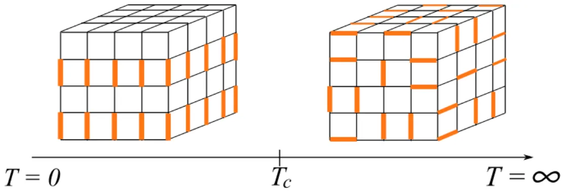
Low Temperature phase At low temperature, the dimers all align to minimize the energy, resulting in a 6-fold degenerate arrangement of dimers in the thermodynamic limit. The asso-ciated local order parameter is the vector :

mα_{(r) = (−1)}rα_n

α(r), (1.22)

where nα(r) is equal to 1 if the related bond is occupied, and 0 otherwise. The factor (−1)rα

takes into account the bipartiteness of the lattice, which will be crucial as we will see in the following. For the six columnar configurations, the local order parameter reads :

M = 1 N ! r m(r) =      ±10 0   ,   _±10 0   ,   00 ±1     . (1.23)

1.2. UNCONVENTIONAL PHASE TRANSITIONS IN DIMER MODELS

High Temperature phase The high-temperature phase is strikingly different compared to its counterparts in Ising-like models. Although no long-range order exists, the correlations between dimers show an algebraic decay :

"dα_(r)dβ_{(0)! =} 4π

Kdim(T )

3rα_rβ_{− δ}αβ_r2

r5 . (1.24)

The coefficient Kdim(T ) is called the stiffness and depends on T . The form of the correla-tions, which are similar to the interaction energy between two electric dipoles, led to the name Coulomb phase for this state of matter. This kind of algebraic liquid is not peculiar to the dimers and has been found in other 3D models, notably in the study of spin ice on pyrochlore lattices [37]. In both cases, the reason for a non exponential decay of the correlations is the pre-sence of a local constraint or conservation law. In the case of the dimers, it is the close-packing condition. For the pyrochlore compounds, it is a constraint on the sum of all spin variables in each tetrahedron (the ”ice rule” [38]). Both cases can be summarized altogether by introducing a fictitious electric field satisfying a Gauss law [37, 39] :

∇ · E(r) = ±1. (1.25)

In our case of interest, the electric field is defined via the occupation number on each bond :

E(r) = (₋₁₎r_{n(r), (1.26)}

so that E always goes from one sublattice to another. It is rather easy to see that the close-packing condition reduces then to (1.25). The bipartiteness of the lattice is of extreme impor-tance here. For insimpor-tance, no Gauss law can be written in the triangular lattice (and corres-pondingly, no algebraic liquid has been found so far). Afterwards, this conservation law and the form of the correlations led some authors to postulate that the Coulomb phase should be characterized in the continuum by a free electrostatic action :

S = K

2 1

d3x E2, (1.27)

which generates the dipolar correlations. The stiffness K is defined through the dimer fluxes :

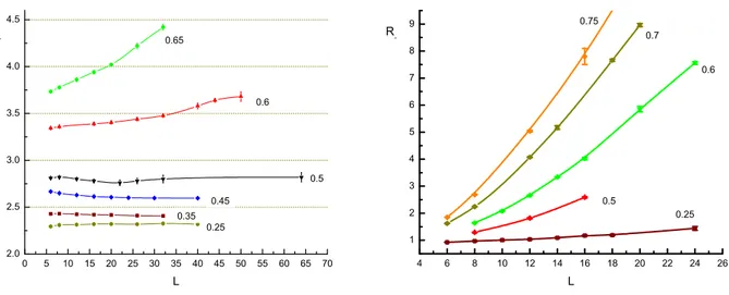
K_dim−1 · L = 1 3("Φ 2 x! + "Φ2y! + "Φ2z!), (1.28) with : Φα = 1 1 Σα E_{· dS,} (1.29)

which are conserved quantities. K_dim−1 acts like an order parameter for the Coulomb phase. On the contrary, it vanishes in the columnar phase since "Φx! = "Φy! = "Φz! = 0. The evolution

of the columnar order parameter M and of K_dim−1 in function of T is shown on Figure 1.10. The critical point Although the low temperature and the high temperature phases seem to be physically very different, simulations pointed unambiguously towards a second-order phase transition at Tc ≈ 1.675. This result was based on various measurements made on the cubic

system for very large sizes (up to L = 128) thanks to the high efficiency of the worm algorithm. In particular :

Fig. 1.10 – Evolution of the columnar order parameter and stiffness in function of the tempe-rature for the dimer model on the cubic lattice [28].

– The histogram of the energy shows no sign of a double-peak structure at Tc as opposed

to what happens in a first order transition.

– The specific heat diverges with the system size at the transition, with a critical exponent

α_{≈ 0.5 to compare with C}v ∼ L3 for a first order transition.

– Different quantities, such as the Binder cumulant B = _'M'M24₍(2 of the columnar order

para-meter, and the product K_dim−1 ·L are scale-invariant at the transition and exhibit a crossing

point.

A finite size scaling (FSS) analysis of the data allowed to extract the set of critical exponents :

ν = 0.50(4)

α = 0.55(6) (1.30)

η = −0.02(5).

This excludes some simple 3d universality classes such as O(2) or O(3). Furthermore, a latter analysis of the probability distribution of the columnar order parameter [40] suggested the emergence of a continuous symmetry at the critical point. Rather than pointing only around the six allowed directions (1.23) of the low temperature phase, the order parameter has a non zero expectation value in all the directions and acquires an enlarged O(3) symmetry at Tc

(see Figure 1.11). So, it seems that the cubic anisotropy drives the system into the columnar phase at low temperature but is absent at the critical point. This supports the idea that the cubic anisotropy is a dangerously irrelevant variable with respect to the transition, in the renormalization group sense. We will come back to this point when analyzing the different theoretical proposals for this transition.

Failure of the ”conventional” scenarios for the dimer transition. The standard pic-ture of phase transitions is based on the concept of order parameter and its long wavelengths fluctuations. Accordingly, to describe a phase transition, it is enough to search for an action expressed as a power series in the order parameter, which respects all the original symme-tries of the problem. In general, this action has a symmetric solution at high temperature, and a non-symmetric one at low temperature. When crossing the critical point, the symmetry

1.2. UNCONVENTIONAL PHASE TRANSITIONS IN DIMER MODELS

Fig. 1.11 – Probability distribution P (Mx, My,|Mz| ≤ 0.03) as a function of Nx and Ny below

(T = 1.66), at (T = 1.673) and above (T = 1.675) the critical temperature for different system sizes [40].

is spontaneously broken. Wilson later argued that this process is renormalized by the ther-mal fluctuations of the order parameter, and that only the leading terms in the power series are relevant for the critical behavior. This is the so-called ”Ginzburg-Landau-Wilson” (LGW) paradigm. Applying this scheme to the dimer transition above, one could propose the action :

S = 1 d3x 2 ! α 3 1 2(∇ · Mα) 2_{+ rM}2 α 4 + u(M4 x + My4+ Mz4) 5 . (1.31)

The last term accounts for the six anisotropic solutions at low T . However, this action fails to capture the physics of the high T phase. In particular, the correlation functions decay expo-nentially above Tc, with a correlation length decreasing to zero at T =∞. That is qualitatively

different from the Coulomb phase, where the correlation length is infinite for any T > Tc.

Mo-reover, perturbative calculations, based on the ε-expansion, predicts a first-order scenario with this action [41, 42] . Clearly, (1.31) does not take into consideration the local conservation law (1.25) and is therefore inadequate for the dimer model.

a ”magnetic” field on the lattice by defining : B(r) = E(r)_{− E}0(r) (1.32) E0(r) = (−1) r 6     1 1 1     . (1.33)

This field is divergence free. The simplest action on the lattice which should generate the correct dipolar correlations is : Z = 1 [Dθ] +∞ ! B(r)=−∞ exp 2 −! r [K 2B 2_{+ iθ(r)(} ∇ · B)] 5 (1.34) Z _∼ 1 [Dθ]exp 2 −_K2 ! r cos(_∇θ) 5 , (1.35)

where the variables θ(r) are the Lagrange multiplier ensuring the divergence free constraint on each site and we used the Villain approximation to derive the second line. The electrostatic action is dual to a three dimensional XY model with an inverted temperature. The disordered phase of the dimer model maps to the ordered phase in the XY language. The Goldstone mode associated with the dual O(2) broken symmetry is the ”photon” gauge field B =∇ × A which

is effectively massless in the Coulomb phase [43, 44]. Nevertheless, there are two problems with the 3d XY duality transform. First, it is unable to establish an equivalence with the columnar phase at low temperature. A suitable redefinition of the electrostatic action, which includes the ”background charges” (₋₁₎r _{of the Gauss law, seems necessary. Secondly, and no least, the} dimer transition is not in the 3d XY class !

1.2.3

Emerging scenarios for generic unconventional phase

transi-tions

Some other unconventional phase transitions

In parallel with these intriguing results on the dimer model, numerical evidences of phase transitions hardly apprehensible within the LGW framework were found in quantum frustrated magnets. One example is given by a ring exchange model on the square lattice which consists of nearest neighbor interactions plus four-spin interactions on the plaquettes [29]. By varying the strength of the ring couplings, a transition between a columnar VBC and a N´eel phase is observed with Quantum Monte Carlo simulations. The numerics support a continuous transition with new critical exponents. That is rather surprising as both phases across the transition are characterized by apparently independent order parameters. A latter study [45] showed that, quite similarly to the dimer model, the probability distribution of the columnar order parameter in the ring-exchange model displays full isotropy near the VBC side of the transition while deep in the VBC phase, it only orientates in the four preferred directions. Another model with unconventional results is the classical O(3) ferromagnet in three dimensions with no topological defects [30]. Classical Heisenberg models in three dimensions allow for non-trivial configurations called ”hedgehogs”. The authors of [30] showed in their study that if

1.2. UNCONVENTIONAL PHASE TRANSITIONS IN DIMER MODELS

these particular configurations are not allowed in the statistical ensemble, this has a radical effect on the properties of the system and in particular on the criticality of the ferromagnetic-paramagnetic transition. Indeed, new critical exponents, different from the O(3) universality class, were calculated. These discoveries led to an intense theoretical activity to overcome the apparent inconsistencies with the description of phase transitions given by the LGW theory. In fact, the conventional theory predicts that if there is a direct transition between two phases with different broken symmetries, it is generically first order. A new theory of critical points is thus necessary to explain the continuous VBC-N´eel transition. That could, in turn, give some possible suggestions for the dimer problem we are focusing on. One of the most promising (and still controversial) theoretical proposal is the deconfined quantum criticality (DQC) scenario. We will review the main arguments supporting this theory, and its possible implications for the dimer transition.

The deconfined quantum criticality scenario

The DQC theory proposes a coherent framework for continuous transitions between phases with different broken symmetries. It mainly assumes the existence of a more fundamental de-gree of freedom than the different order parameters of the two phases. These dede-grees of freedom are not directly observable in the phases because they are confined, i.e they do not propagate freely like independent particles. We already saw an example of such elementary block with the spinons of the VBC phase (Figure 1.5). One could also think of the quarks in a nucleus. It is argued in the DQC scenario that exactly at the critical point, this elementary blocks should deconfine. The deconfined quantum critical point has thus very different properties from the two phases it separates. Let us review the construction leading to the DCP.

To determine the properties of antiferromagnets, one can prospect microscopic Hamiltonians like the Heisenberg model. Alternatively, it is also possible to begin with a continuum approach able to reproduce the long wavelength fluctuations of the order parameter. This roadmap exists and is given by the non-linear sigma model. There, the fluctuations of the staggered magneti-zation m(r, t) (the N´eel order parameter) on a square lattice are subject to the action :

S = 1 d3x 1 2g(∇µm) 2_{+ iS}! r A[m(r, t)](−1)r. (1.36)

where g is a coupling constant, and S is the magnitude of the spin. The vector m has norm 1. The first term can be derived from a continuum version of the Heisenberg Hamiltonian (1.1) using a basis of coherent states [46]. In the process, one goes to imaginary time to obtain a classical action in three dimensions. The coupling constant g is inversely proportional to S. The second term is more subtle : it is the sum of the Berry phases of each spin. The Berry phase is equal to the area on the unit sphere enclosed by the path that makes a spin through time (Figure 1.12)[47] . This geometrical phase derives from the coherent state representation of the spin operators. The approximations underpinning the non-linear sigma model (1.36) are valid for large S only. In practice, it has proved to give results in quantitative agreement with experiments even for S = 1

2 materials [48, 49].

The action (1.36), without the Berry phase term, can be studied within the renormalization group approach in perturbation theory. A 2 + ε expansion indicates a phase transition in three dimensions between a N´eel state at low coupling and a disordered state for g > gc. Non

Fig. 1.12 – Representation of the Berry phase. At each site, the N´eel order parameter draws a closed path on the unit sphere through time. The Berry phase is given by the area enclosed by the path.

frustrated microscopic models such as the Heisenberg model on a square lattice always fall into the antiferromagnetic side of the phase diagram, as predicted by the linear spin-wave theory. If one adds frustrating interactions, the value of g should increase and eventually lead to a disordered phase at zero temperature.

When the (imaginary) Berry phase term is included, the picture changes radically. Let us briefly resume the mechanism in hold here, which was first developed by Haldane [50]. The two crucial ingredients in his analysis are the presence of tunneling events during the time evolution of the system, the instantons, and the Berry phase term which can lead to destructive interferences between these events. For smooth configurations of the field m(r, t) (i.e m(r, t) is continuous and derivable through space and time), Haldane first argues that the total Berry phase is zero. This is understandable if one remembers that the total Berry phase of a one dimensional spin system is given by the skyrmion number :

Qxt= 1

4π 1

dxdt_∇tm· (m × ∇xm) ∈ Z. (1.37)

which is an integer. Here, we assume that space and time have been compactified : limr_→∞m(r, t) = lim_t→∞m(r, t) = m0 so that the action (1.36) remains finite. This number is very similar to the winding numbers in the quantum dimer models. It indexes topological sectors of spin confi-gurations. The existence of different topological sectors is ascertained by the non triviality of the second homotopy group of the sphere :

Π2(S2) =Z. (1.38)

Because of the staggered factor in the imaginary part of (1.36), the total Berry phase on a square lattice is simply given by the alternated sum of the Berry phases of each (x, t) plane :

S_BPtot = i2πS!

y

(−1)y_Qxt_{(y) (1.39)}

If the configuration is smooth through time and space, Qxt _{is necessarily the same for all (x, t)}