Metal fluxes at the water sediment interface of shallow mine tailings ponds, Heathe Steele mines, New Brunswick.

Texte intégral

(1)METAL FLUXES AT THE WATERSEDIMENT INTERFACE OF SHALLOW MINE TAILINGS PONDS, HEATH STEELE MINE, NEW BRUNSWICK.

(2)

(3) METAL FLUXES AT THE WATER-SEDIMENT INTERFACE OF SHALLOW MINE TAILINGS PONDS, HEATH STEELE MINE, NEW BRUNSWICK. Report written for Philippe Poirier et Julie Gravel (SNC-Lavalin). Claude Fortin, Lise Rancourt and Peter G.C. Campbell. Institut national de la Recherche scientifique, INRS-ETE 490, rue de la Couronne, Québec (Québec), G1K 9A9. Research report R-772. November 2004. iii.

(4) © Claude Fortin, 2004. iv.

(5) ACKNOWLEDGMENTS Accomplishment of this work was possible through the collaboration of numerous persons that we wish to acknowledge. Divers and lab technicians: René Rodrigue, Pierre Marcoux, Michelle Geoffroy Bordeleau and Pauline Fournier Lab supervisor: Stéfane Prémont Heath Steele Mine site manager: Norman Morris. v.

(6) vi.

(7) ABSTRACT Dissolved water constituent concentration profiles were established at the surface water – sediment interface in the three submerged tailings cells at the Heath Steele Mine (NB, Canada) using in situ dialysis peepers and trace metal clean techniques. Dissolved surface water trace element concentrations ranged from the low nanomolar level for cadmium (~ 10-9 M) to the high nanomolar level for zinc (~10-7 M). Concentrations decreased in the order: Zn > Ni > Cu > Pb ~ As ~ Se > Tl > Cd. Overall, dissolved porewater metal concentrations increased with sediment depth in the lower and upper cells and remained relatively unchanged in the north cell. From the established profiles, diffusional fluxes of copper, lead, zinc, nickel, cadmium, arsenic and thallium ions at the water-sediment interface were calculated. Comparison of results from duplicate peepers demonstrated an important spatial variability within each cell. Fluxes were nevertheless mostly negative, indicating a release of metals from the sediments to the water column. These fluxes were however quite low and would be expected to reverse in direction if more reducing conditions appear in the sediments as the tailings age.. vii.

(8)

(9) TABLE OF CONTENTS ACKNOWLEDGMENTS.............................................................................................................v TABLE OF CONTENTS .............................................................................................................ix LIST OF FIGURES......................................................................................................................xi LIST OF TABLES........................................................................................................................xi CHAPTER 1 : Introduction and objectives ................................................................................1 1.1 INTRODUCTION ............................................................................................................... 1 1.2 OBJECTIVES...................................................................................................................... 1 1.3 MILESTONES .................................................................................................................... 1 CHAPTER 2 : Methods ................................................................................................................3 2.1 STUDY SITE....................................................................................................................... 3 2.1.1 Heath Steele Mine ...................................................................................................... 3 2.1.2 Sampling stations ....................................................................................................... 3 2.2 SAMPLING......................................................................................................................... 4 2.2.1 Sediment core sampling ............................................................................................. 4 2.2.2 Porewater sampling ................................................................................................... 5 2.3 MEASUREMENTS............................................................................................................. 6 2.3.1 Sediment porosity ....................................................................................................... 6 2.3.2 Dissolved trace metals and major cations ................................................................. 6 2.3.3 Dissolved major anions.............................................................................................. 6 CHAPTER 3 : Results and Discussion ........................................................................................7 3.1 POREWATER CONCENTRATION PROFILES .............................................................. 7 3.1.1 pH ............................................................................................................................... 7 3.1.2 Major anions .............................................................................................................. 7 3.1.3 Major cations ............................................................................................................. 7 3.1.4 Iron and manganese ................................................................................................. 10 3.1.5 Lead, cadmium and zinc........................................................................................... 10 3.1.6 Copper, nickel and arsenic....................................................................................... 10 3.1.7 Selenium and thallium.............................................................................................. 15 3.2 SURFACE WATER CONCENTRATIONS ..................................................................... 15 3.3 ELEMENT FLUXES ACROSS THE WATER-SEDIMENT INTERFACE ................... 16 3.4 ESTIMATED ELEMENT OUTPUT ON A DAILY BASIS............................................ 17 3.5 SOLUBILITY CALCULATIONS .................................................................................... 18 CHAPTER 4 : Conclusion ..........................................................................................................21 BIBLIOGRAPHY........................................................................................................................23. ix.

(10)

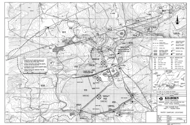
(11) LIST OF FIGURES Figure 2.1: Topographic map and sampling site locations (×)..................................................3 Figure 2.2: Schematic illustration of in situ porewater peepers used........................................4 Figure 3.1: Duplicate pH and dissolved sulphate and chloride concentration profiles at the sediment – water interface in all three sampled cells. ................................8 Figure 3.2: Duplicate dissolved calcium, magnesium and potassium concentration profiles at the sediment – water interface in all three sampled cells. ................................9 Figure 3.3: Duplicate dissolved sodium, iron and manganese concentration profiles at the sediment – water interface in all three sampled cells. Values below detection limits were not plotted. Note the change in scale for Fe in the upper cell. ..................................................................................................................................11 Figure 3.4: Duplicate dissolved zinc, cadmium and lead concentration profiles at the sediment – water interface in all three sampled cells. Values below detection limits were not plotted. ....................................................................................12 Figure 3.5: Duplicate dissolved copper, nickel and arsenic concentration profiles at the sediment – water interface in all three sampled cells. Note change in scale and break in x-axis for As in the upper cell profile. ........................................................13 Figure 3.6: Duplicate dissolved selenium and thallium concentration profiles at the sediment – water interface in all three sampled cells. .....................................................14 Figure 3.7: Ion activity products (on a log scale) for the precipitation of Pb(OH)2 (s) calculated for each peeper (white or black filled symbols) and each cell using two scenarios. Scenario 1 (circles) assumed equilibrium with atmospheric CO2 (g) whereas scenario 2 (squares) neglected the presence of dissolved carbonates. Oversaturation is reached when the log IAP > log Ksp (i.e., to the left of the vertical line drawn at -19.96)........................................................19. LIST OF TABLES. Table 3.1: Average measured constituent (± standard deviation) in the peeper chambers above the sediment (n = 6). ..................................................................15 Table 3.2: Average measured porosity on sediment cores (n = 3) and computed diffusive fluxes (JD) for each peeper sampled. .....................................................17 Table 3.3: Mean sediment metal export to the water column and estimated dissolved metal export from each cell. .................................................................18. xi.

(12)

(13) CHAPTER 1 : Introduction and objectives 1.1 INTRODUCTION Many commercially exploited ores contain a large proportion of sulphides, present mainly as pyrite (FeS2). Pyrite-containing tailings produced by mining can be oxidized when exposed to the atmosphere and rainfall, generating large amounts of sulphuric acid (generally termed acid mine drainage or AMD). The major oxidants of pyrite are dissolved oxygen (DO) and, once the oxidation process has been initiated, Fe3+. In this latter process, the rate-limiting step of the oxidation process is the oxidation of Fe2+ to Fe3+, which is catalyzed by microorganisms (Singer and Stumm, 1970). The resulting acidic solution can leach metals from the tailings, constituting a threat to the receiving environment. One way to limit DO diffusion into the tailings is by using physical barriers. Because of its economic and environmental relevance, the utilization of water covers for the prevention of AMD has been considered. Underwater disposal attenuates the input of DO to tailings, given the low diffusion coefficient and solubility of oxygen in overlying and interstitial water. In addition, anoxic conditions should inhibit the microbial catalysis associated with the oxidation process. Mine tailings at the Heath Steele Mine were sheltered from ambient oxygen by a shallow water cover in an attempt to minimise sulphur oxidation and acid mine drainage. The effectiveness of water covers have been questioned and assessed in the past (MEND, 1989; Pedersen et al., 1993; Vigneault et al., 2001). Metal mobilisation from the deposited tailings might result from combination of several factors (e.g., sediment resuspension resulting from wind-induced turbulence, or establishment of a periphyton layer on the tailings surface, the photosynthetic activity of which would constitute a localized source of DO). Such mobilisation can be analytically determined using porewater peepers to determine dissolved metal concentration gradients and thus calculate element fluxes in the dissolved phase at the sediment-water interface. 1.2 OBJECTIVES Mine tailings at the Heath Steele Mine are known to contain a considerable quantity of metals, notably Zn, Cu and Pb. To evaluate the effectiveness of the shallow water cover in stabilising the mine tailings at Heath Steele Mine, water column and porewater metal concentrations (Zn, Cu and Pb) were determined using in situ equilibrated peepers and element fluxes were determined for all three sampling sites. 1.3 MILESTONES 1. July 2004. Install 6 sediment porewater peepers at sites selected by SNC-Lavalin (3 sites ; 2 peepers / site). The degassed ultrapure water filled peeper chambers are 1 cm apart vertically, have a volume about 4 mL, and are two cells wide. All peepers are.

(14) gently inserted by experienced divers. At each station obtain three sediment samples using minicorers in order to determine the superficial sediments’ porosity. 2. August 2004. Recover peepers after a period of time long enough to reach equilibrium (3 weeks). 3. August – September 2004. In the four chambers above and below the water – sediment interface, determine pH, major cations, major anions and metals (Cu, Pb, Zn, and others provided concentrations are high enough; e.g.: Fe, Mn, Cd, Ni) concentrations. 4. September – October 2004. From the dissolved metal profiles (i.e. the concentration gradient) and sediment porosity data, calculate fluxes in Cu, Zn and Pb across the water – sediment interface for each peeper. 5. Preliminary report due end of October 2004. 6. Final report due early November 2004.. 2.

(15) CHAPTER 2 : Methods 2.1 STUDY SITE 2.1.1. Heath Steele Mine. The Heath Steele Mine is located in New Brunswick, approximately 60 km southwest of Bathurst, NB. The submerged mine tailings are separated in three cells: Upper, North and Lower cells (Figure 1). The Heath Steele Mine mining and milling activities were first developed in the 50s but are no longer in operation. The mined ores consisted mainly of base metal sulphides (Zn, Pb, Cu and Ag; Beak, 1998). 2.1.2. Sampling stations. One sampling station was selected for each cell (Figure 2.1). All stations were ~ 10 m away from the shore and two peepers were installed at each site, ~ 3 m apart. Peepers were installed on July 21st 2004 and recovered on August 11th 2004. Weather conditions were favourable on both occasions (no rain).. Figure 2.1: Topographic map and sampling site locations (×).

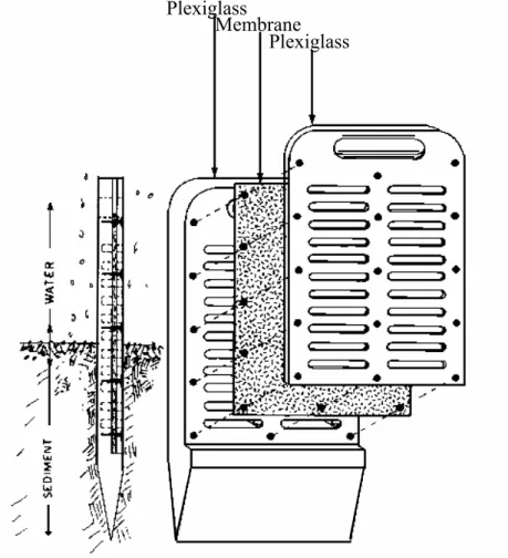
(16) 2.2 SAMPLING All sampling material had been previously decontaminated using diluted nitric acid (≥ 24 hours in 10% HNO3 v/v; ACS grade), then thoroughly rinsed with ultrapure water (resistivity ≥ 18 MΩ cm) and dried under a class 100 laminar flow hood. 2.2.1. Sediment core sampling. Sediment cores (in triplicates) were initially taken at each sampling station before peepers were installed to determine porosity for sediment flux calculations purposes. Cores were obtained by divers using a 78 mm diameter PVC cylinder and extruded. The first four centimetres were individually sampled into 100 mL pre-weighed polypropylene containers. Samples were subsequently weighed before and after they were dried in an oven at 60°C for 3 days. Water content was then computed from the difference in weight. Plexiglass Membrane Plexiglass. Figure 2.2: Schematic illustration of in situ porewater peepers used. 4.

(17) 2.2.2. Porewater sampling. 2.2.2.1 In situ peepers Figure 2.2 illustrates the different parts of a porewater peeper similar to those used in this study. Porewater peepers are multi-chambered equilibrium dialysis samplers made of polymethylmethacrylate (acrylic, Plexiglas). There are two columns of 4 mL volume chambers providing a 1 cm vertical resolution. Decontaminated peepers are first deoxygenated by storing them in a gas-tight container purged with nitrogen gas for a month. They are then immersed in ultrapure water and covered by semi-permeable polysulfone membrane of 0.2 µm porosity (GelmanTM HT-200). An acrylic cover is then fixed onto the membrane with stainless steel screws while carefully avoiding entrapment of any air bubbles. The peepers are then returned to the gas-tight container under a nitrogen gas atmosphere for a minimum of two weeks. This procedure removes virtually all oxygen trapped in the acrylic and in the water that could oxidize redox sensitive species in reducing environments such as those usually found in sediments (Carignan et al. 1994). Once in place, external solutes will diffuse through the membrane into the cavities until equilibrium is reached (i.e. when external and internal concentrations are identical). The water composition in the chambers is then considered representative of the immediate surrounding porewaters and does not require filtering. 2.2.2.2 Peepers deployment and recovery Peepers were rapidly removed from their nitrogen gas environment and gently inserted into the sediments in a vertical position by divers. Two peepers were installed at each of the three sampling stations. After three weeks, the peepers were localised and visually inspected in situ before their removal to determine the exact location of the sediment-water interface. Four cells above and below the interface were sampled immediately after removal of the peepers in order to obtain an 8 cm vertical profile. Three subsamples for each depth were taken for the determination of: i) dissolved metals and cations; ii) dissolved anions; and iii) pH. A first 4 mL subsample (representing a complete cell volume) was removed at each depth by carefully poking the membrane with a clean pipette tip and slowly pipetting the cell content. The sample was then injected into an acid-washed pre-acidified 4 mL HDPE container (40 µL of HNO3 2 M; Seastar - Trace Metal Grade; added as a preservative). The samples were then stored on ice and refrigerated upon arrival at the lab until they were analysed for their Na, K, Ca, Mg, Fe, Mn, Zn, Cd, Pb, Cu, Ni, As, Se and Tl content. A second subsample of 3 mL was then collected similarly from the other peeper column. The samples were placed into new 4 mL HDPE containers that had been thoroughly washed with ultrapure water. The samples were then stored on ice and refrigerated upon arrival at the lab until they were analysed for Cl, SO4, PO4 and NO3. Ultrapure water was sampled in a similar manner and treated as samples to obtain field blanks for both cations and anions subsequent analyses. A final 1 mL subsample was then used to determine pH. pH was measured on-site within 30 minutes of the peepers’ removal using a combined semimicro pH electrode and field pH-meter. 5.

(18) (Fisher Accumet gel electrode with Ag/AgCl reference). Drift was noted before and after sampling each peeper and recalibrated when offset was above 0.1. 2.3 MEASUREMENTS Detection limits (LD) were calculated by multiplying by 3 the standard deviation of ten measurements of a sample of low concentration. 2.3.1. Sediment porosity. Sediment porosity (φ) was calculated using equation 2.1: (2.1). φ=. VH 2O Vt. where VH2O = volume of water in the sediments (mL) Vt = total sediment volume (mL) And Vt was obtained from equation 2.2: (2.2). Vt = VH 2O + Vsed. where Vsed = volume occupied by dry sediments (mL) Finally, Vsed was computed using equation 2.3: (2.3). Vsed =. m sed ρ sed. where msed = mass of dry sediments (g) ρsed = density of dry sediments (2.5 g/mL; Lerman 1979) 2.3.2. Dissolved trace metals and major cations. Dissolved trace metals and major cations concentrations in the peepers’ chambers were determined by inductively coupled plasma optical emission spectrometry (ICP-OES; Vista AX CCD) and by inductively coupled plasma mass spectrometry (ICP-MS; Thermoelemental; X7). Quality control was ensured by frequent analyses of analytical blanks, sample duplicates and reference material. Detection limits obtained were: 0.5 µM Ca; 0.2 µM Mg; 0.4 µM Na; 0.4 µM Fe; 0.04 µM Mn; 0.06 µM Zn; 0.1 nM Cd; 0.1 nM Pb; 0.8 nM Cu; 11 nM Ni; 1.5 nM As; 6 nM Se; and 0.04 nM Tl. 2.3.3. Dissolved major anions. Total dissolved concentrations of PO4, NO3, F, SO4 and Cl were determined by ion chromatography (Dionex IONPAC AS14 Suppressed Conductivity ASRS-II). Detection limits for these constituents were: 0.1 mM PO4; 0.15 mM NO3; 0.5 µM F; 1 µM Cl ; and 3 µM SO4.. 6.

(19) CHAPTER 3 : Results and Discussion 3.1 POREWATER CONCENTRATION PROFILES. Vertical profiles of different dissolved constituents measured at the water-sediment interface of all three cells were plotted (figures 3.1 – 3.6). Fluoride, nitrate and phosphate concentrations were either below the detection limit or were less than three times this limit. These profiles were thus omitted. 3.1.1. pH. The highest surface water pH (range: 8.7 – 9.0) was observed, not surprisingly, in the north cell, the closest to the water neutralising plant (Figure 3.1). In the cells below, surface water pH was roughly an order of magnitude less (upper cell pH range: 7.7 – 7.9; lower cell pH range: 7.6 – 8.0). In the porewater, pH was even higher in the north cell with a range of 9.0 – 9.5 (perhaps the tailings were limed before being submerged) whereas in the lower cell pH was closer to neutrality (range: 7.3 – 7.9), with little difference with its overlying water. On the other hand, the porewater pH of the upper cell was more acidic than the water column with a minimum value of 6.3. 3.1.2. Major anions. One can tell from the sulphate profiles (Figure 3.1) that the tailings were submerged only recently (actually between 1997 and 2001; J. Gravel, pers. comm.) as no decrease in sulphate in the sediments was observed (as one would expect in natural water bodies, for example). As the sediments age, porewater sulphate concentrations should decrease, indicating reduction to sulphides. In contrast, the sediments of the lower cell are obviously acting as a source of sulphate to the surface water whereas in the other two cells, no gradients appear, indicating that for the moment the sediments and the water are at steady state. Indeed, the tailings of the lower cell had undergone some oxidation as they were exposed to the atmosphere for 8 months in 2001 (J. Gravel, pers. comm.). Dissolved chloride profiles (Figure 3.1) were on the other quite uniform in and above the sediments, as expected from a conservative anion, with concentrations around 0.2 mM. 3.1.3. Major cations. Similar to sulphate, gradients in dialysable Ca, Mg, K and Na (Figures 3.2 and 3.3) were only noticeable in the sediments of the lower cell, with an important local spatial heterogeneity (duplicates do not overlap for almost all elements analysed in this cell’s peepers). The tailings from this cell were the last to be submerged (J. Gravel, pers. comm.) and background cations are likely still diffusing toward the surface waters. Note that the Ca concentrations in the lower cell surface waters are also the lowest ones. The origin of the cations might come from residual lime still dissolving at a greater rate than in the other cells or from the old tailings area (draining into the upper cell) or due to the original upper cell tailings composition..

(20) 2-. 0. [SO4 ] (mg/L) 500 1000. -. 1500. 0. 2. [Cl ] (mM) 4 6. 8. 10. -4 -3. Depth (cm). Lower cell. -2 -1 0 1 2 3 4 6. 7. 8. 9. 10. 0. 5. 10. 15. 0.0. 0.1. 0.2. 0.3. 6. 7. 8. 9. 10. 0. 5. 10. 15. 0.0. 0.1. 0.2. 0.3. 6. 7. 8. 9. 10. 0. 5. 10. 15. 0.0. 0.1. 0.2. 0.3. -4 -3. Depth (cm). Upper cell. -2 -1 0 1 2 3 4. -4 -3. Depth (cm). North cell. -2 -1 0 1 2 3 4 2[SO4 ]. pH. (mM). -. [Cl ] (mM). Figure 3.1: Duplicate pH and dissolved sulphate and chloride concentration profiles at the sediment – water interface in all three sampled cells.. 8.

(21) Ca (mg/L) 0. Mg (mg/L). 100 200 300 400 500 600. 0. 10. 20. 30. 0. 5. K (mg/L) 10 15. 20. -4 -3. Depth (cm). Lower cell. -2 -1 0 1 2 3 4 0. 5. 10. 15. 0.0. 0.5. 1.0. 1.5 0. 100. 200. 300. 400. 500. 0. 5. 10. 15. 0.0. 0.5. 1.0. 1.5 0. 100. 200. 300. 400. 500. 0. 5. 10. 15. 0.0. 0.5. 1.0. 1.5 0. 100. 200. 300. 400. 500. -4 -3. Depth (cm). Upper cell. -2 -1 0 1 2 3 4. -4 -3. Depth (cm). North cell. -2 -1 0 1 2 3 4. Ca (mM). Mg (mM). K (µM). Figure 3.2: Duplicate dissolved calcium, magnesium and potassium concentration profiles at the sediment – water interface in all three sampled cells.. 9.

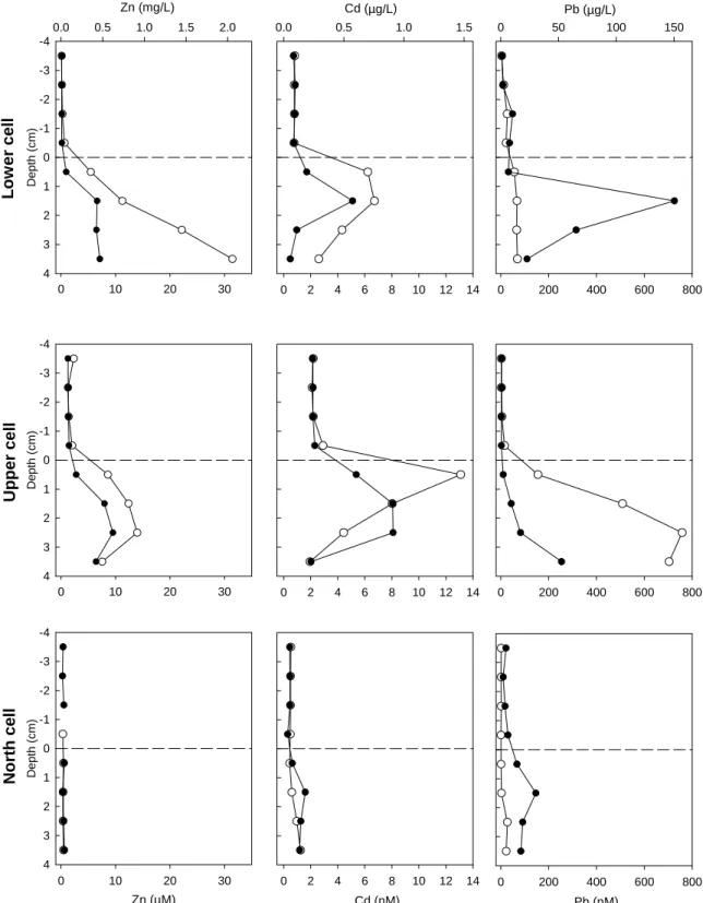
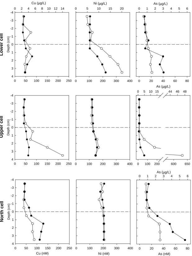
(22) 3.1.4. Iron and manganese. Similar to sulphate, iron and manganese are redox sensitive elements. Indeed, the more soluble Fe(II) and Mn(II) species can be oxidised to less soluble Fe(III) and Mn(III, IV) species in the presence of oxygen. We thus expect greater dissolved concentrations deeper in the sediments where oxygen is scarce thus favouring the +2 state. Such typical profiles were observed in the lower and upper cells but not in the north cell (Figure 3.3). In this latter cell, the solubility of Fe(II) might have been limited by the high pHs observed in these sediments favouring the precipitation of Fe(II) hydroxides (solubility constant Ksp Fe(OH)2 (s) = 10-15.1, Morel and Hering, 1993; at pH 8.5, the solubility of Fe(OH)2 (s) in pure water is 2 µM). Note that the dissolved iron concentrations are much higher in the lower porewater samples in the upper cell (Figure 3.3; note change in scale for Fe in the upper cell) where pH was lowest (Figure 3.1). 3.1.5. Lead, cadmium and zinc. Overall, porewater concentrations of these metals were in the order: Zn > Pb > Cd (Figure 3.4). The lowest concentrations were observed in the north cell where no substantial gradients could be detected (the sediments are thus not an important source of these metals for the surface waters). In contrast, notable gradients were observed in the other two cells, again with important spatial variability (e.g., see Pb profiles in the lower and upper cells; Figure 3.4). Lead gradients at the sediment – surface water interface were negligible in the lower cell. Moreover, in one of the peepers, there seems to be a source of dissolved lead ~1.5 cm below the sediments but compensated by two sinks, one immediately below the surface water and another one deeper in the sediments, inducing a downward diffusion flux from the source. In the upper cell, a more gradual increase in dissolved lead was observed with depth. For Cd, dissolved porewater concentrations peaked just below the surface of the upper and lower cells, suggesting a diffusion both upward (to the surface waters) and below (deeper into the sediments) a source in the superficial sediments. The highest dissolved Cd surface concentrations were in the upper cell (~2 nM), roughly twice that of the lower cell and four times that of the north cell. Finally, the sediments of the lower and upper cells were also acting as a source of Zn for the surface waters but the concentrations are relatively low (in fact very close to the 0.1 µM detection limit in the lower cell) although in one peeper of the lower cell concentrations above 30 µM were reached in the fourth cm of the sediments. 3.1.6. Copper, nickel and arsenic. Porewater Cu concentrations increased with depth with some local heterogeneity (see upper cell profile; Figure 3.5). In all profiles, gradients indicated an upward diffusion of Cu from the sediments, albeit of an apparently low amplitude. Ni concentrations were quite high both above and below the sediment – overlying water interface. Only the lower cell profile suggested an important diffusional gradient toward the surface water. No consistent large gradients in As were observed at the sediment – water interface but dissolved concentrations were substantially higher in the sediments, especially in one of the peepers of the upper cell.. 10.

(23) 0. 10. Na (mg/L) 20. 30. 0.0. 0.5. Fe (mg/L) 1.0 1.5. 2.0. 2.5. Mn (mg/L) 10. 0. 5. 15. 0. 100. 200. 300. 0. 100. 200. 300. 0. 100. 200. 300. -4 -3. Depth (cm). Lower cell. -2 -1 0 1 2 3 4 0.0. 0.5. 1.0. 1.5. 0. 10. 20. 30. Fe (mg/L) 20 30. 0. 10. 0. 200. 400. 0.0. 0.5. 1.0. 40. 40. 50. -4 -3. Depth (cm). Upper cell. -2 -1 0 1 2 3 4 0.0. 0.5. 1.0. 1.5. 600. 800. 1000. Fe (mg/L) 1.5. 2.0. 2.5. -4 -3. Depth (cm). North cell. -2 -1 0 1 2 3 4 0.0. 0.5. 1.0. 1.5. 0. 10. Na (mM). 20. Fe (µM). 30. 40. Mn (µM). Figure 3.3: Duplicate dissolved sodium, iron and manganese concentration profiles at the sediment – water interface in all three sampled cells. Values below detection limits were not plotted. Note the change in scale for Fe in the upper cell.. 11.

(24) Zn (mg/L) 0.0. 0.5. 1.0. Cd (µg/L) 1.5. 2.0. 0.0. 0.5. 1.0. 1.5. 0. Pb (µg/L) 100. 50. 150. -4 -3. Depth (cm). Lower cell. -2 -1 0 1 2 3 4 0. 10. 20. 30. 0. 2. 4. 6. 8. 10. 12. 14. 0. 200. 400. 600. 800. 0. 10. 20. 30. 0. 2. 4. 6. 8. 10. 12. 14. 0. 200. 400. 600. 800. 0. 10. 20. 30. 0. 2. 4. 6. 8. 10. 12. 14. 0. 200. 400. 600. 800. -4 -3. Depth (cm). Upper cell. -2 -1 0 1 2 3 4. -4 -3. Depth (cm). North cell. -2 -1 0 1 2 3 4. Zn (µM). Cd (nM). Pb (nM). Figure 3.4: Duplicate dissolved zinc, cadmium and lead concentration profiles at the sediment – water interface in all three sampled cells. Values below detection limits were not plotted.. 12.

(25) Cu (µg/L) 0. 2. 4. 6. 8. Ni (µg/L) 10 12 14. 0. 5. 10. 0. 100. 15. 20. 0. As (µg/L) 2 3 4. 1. 5. 6. -4 -3. Depth (cm). Lower cell. -2 -1 0 1 2 3 4 0. 50. 100. 150. 200. 250. 200. 300. 400. 0 0. 20. 40. 60. As (µg/L) 10 15 44. 5. 80. 46. 48. -4 -3. Depth (cm). Upper cell. -2 -1 0 1 2 3 4 0. 50. 100. 150. 200. 250. 0. 100. 200. 300. 400. 0. 0. 100. 1. 200. 2. 600. As (µg/L) 3 4. 650. 5. 6. -4 -3. Depth (cm). North cell. -2 -1 0 1 2 3 4 0. 50. 100. 150. 200. 250. 0. 100. Cu (nM). 200. Ni (nM). 300. 400. 0. 20. 40. 60. 80. As (nM). Figure 3.5: Duplicate dissolved copper, nickel and arsenic concentration profiles at the sediment – water interface in all three sampled cells. Note change in scale and break in x-axis for As in the upper cell profile.. 13.

(26) 0.0 -4. 0.5. Se (µg/L) 1.0. 1.5. 0.0. Tl (µg/L) 1.5. 0.5. 1.0. 2.0. 2.5. -3. Depth (cm). Lower cell. -2 -1 0 1 2 3 4 0. 5. 10. 15. 20. 25. 0. 2. 4. 6. 8. 10. 12. 0. 5. 10. 15. 20. 25. 0. 2. 4. 6. 8. 10. 12. 0. 5. 10. 15. 20. 25. 0. 2. 4. 6. 8. 10. 12. -4 -3. Depth (cm). Upper cell. -2 -1 0 1 2 3 4. -4 -3. Depth (cm). North cell. -2 -1 0 1 2 3 4. Se (nM). Tl (nM). Figure 3.6: Duplicate dissolved selenium and thallium concentration profiles at the sediment – water interface in all three sampled cells.. 14.

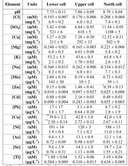
(27) 3.1.7. Selenium and thallium. Selenium profiles (Figure 3.6) were somewhat incoherent, most probably due to inherent analytical variability close to the detection limit (6 nM). Thallium profiles (Figure 3.6) indicated a slight increase in dissolved concentrations in the sediments, especially in one of the peepers of the lower cell. 3.2 SURFACE WATER CONCENTRATIONS. Since the surface water above 1 cm from the sediment interface seemed to be well-mixed (no major evident gradients with perhaps the exception of Pb), the data from the top three chambers of both peepers in each cell were pooled and are presented in Table 3.1. Table 3.1: Average measured constituent (± standard deviation) in the peeper chambers above the sediment (n = 6). Element. Units. Lower cell. Upper cell. North cell. 7.75 ± 0.11 7.86 ± 0.09 8.79 ± 0.04 0.193 ± 0.007 0.170 ± 0.006 0.208 ± 0.004 (mM) 6.9 ± 0.2 6.0 ± 0.2 7.4 ± 0.1 (mg·L-1) 5.42 ± 0.06 6.44 ± 0.05 11.54 ± 0.05 [SO4] (mM) 521 ± 6 618 ± 5 1108 ± 5 (mg·L-1) 5.27 ± 0.20 7.28 ± 0.30 12.52 ± 0.21 [Ca] (mM) 211 ± 8 292 ± 12 502 ± 9 (mg·L-1) 0.248 ± 0.021 0.165 ± 0.003 0.221 ± 0.006 [Mg] (mM) 6.0 ± 0.5 4.01 ± 0.08 5.4 ± 0.2 (mg·L-1) 53.2 ± 5.5 43.6 ± 0.5 65.8 ± 8.5 [K] (µM) 2.1 ± 0.2 1.70 ± 0.02 2.6 ± 0.3 (mg·L-1) 0.360 ± 0.015 0.262 ± 0.006 0.334 ± 0.012 [Na] (mM) 8.3 ± 0.3 6.0 ± 0.1 7.7 ± 0.3 (mg·L-1) 2.60 ± 0.54 0.19 ± 0.04 0.72 ± 0.02 [Mn] (µM) 143 ± 30 10 ± 2 39 ± 1 (µg·L-1) * 0.15 ± 0.06 1.48 ± 0.41 0.39 ± 0.13 [Zn] (µM) (mg·L-1) 0.010 ± 0.004 0.097 ± 0.027 0.025 ± 0.008 0.80 ± 0.04 2.16 ± 0.03 0.49 ± 0.03 [Cd] (nM) (µg·L-1) 0.090 ± 0.004 0.243 ± 0.003 0.055 ± 0.003 17 ± 17 3.1 ± 0.9 8.7 ± 9.2 [Pb] (nM) 3.6 ± 3.7 0.64 ± 0.20 1.8 ± 1.9 (µg·L-1) ** 39.0 ± 2.2 42.8 ± 1.8 42.0 ± 1.8 [Cu] (nM) 2.72 ± 0.12 2.67 ± 0.11 (µg·L-1) **2.58 ± 0.14 101 ± 14 120 ± 3 188 ± 13 [Ni] (nM) 5.9 ± 0.8 7.1 ± 0.2 11.0 ± 0.8 (µg·L-1) 9.6 ± 1.3 13.1 ± 0.9 12.1 ± 1.6 [As] (nM) 0.72 ± 0.09 0.98 ± 0.07 0.91 ± 0.12 (µg·L-1) 9.6 ± 3.9 14.3 ± 1.0 19.7 ± 2.6 [Se] (nM) 0.76 ± 0.31 1.13 ± 0.08 1.55 ± 0.21 (µg·L-1) ** 1.88 ± 0.04 1.52 ± 0.06 3.10 ± 0.04 [Tl] (nM) -1 (µg·L ) 0.384 ± 0.009 0.310 ± 0.013 0.634 ± 0.009 * Data for one peeper only (thus n = 3). In the second peeper, values were all below detection limit (0.1 nM). **One suspicious outlier concentration was ignored (thus n = 5). pH [Cl]. 15.

(28) Dissolved surface water trace element concentrations thus decreased in the order: Zn > Ni > Cu > Pb ~ As ~ Se > Tl > Cd. 3.3 ELEMENT FLUXES ACROSS THE WATER-SEDIMENT INTERFACE. Calculations of diffusive flux do not take into account any biological activity such as bioturbation and bioirrigation that might have affected local profiles. Considering that very little sediment life was observed, the assumption that fluxes are regulated solely by diffusion is reasonable. Any turbulence and resuspension of the sediments caused by wind action was also neglected and thus, we only considered diffusive fluxes. Under steady-state conditions, the diffusive flux of a metal M (JDM) at the water-sediment interface is defined by Fick’s law: (3.1) où. J DM = - φ D eff. d[M ] dx. φ: sediment porosity (calculated using equation 2.1) d[M]/dx: concentration gradient (mol/cm4) Deff : effective ion diffusion coefficient (cm2/s). The concentration gradient (d[M]/dx) can be obtained from concentration profiles at the watersediment interface (Figures 3.1 – 3.6). It can be estimated for each profile generally using the first data points above and below the interface. Deff is the effective ion diffusion coefficient in water (wDt) corrected for tortuosity (θ), temperature and, when necessary, for electric effects. Boudreau (1997) gives a series of relationships between θ and φ for different sediment types. Here, equation 3.2 was used to correct for tortuosity: (3.2). Deff = φ2 · wDt. where wDt = ion diffusion coefficient for a given chemical species (cm2/s) Combining equations 3.1 and 3.2 gives: (3.3). J DM = - φ 3. w. Dt. d[M ] dx. where wDt represents the coefficient of diffusing species. We ought to know what the species distribution is for a given element and thus select appropriate coefficients. However, such level of exactitude is not possible in the present circumstances as the complete species distribution is (partially) unknown and diffusion coefficients are not available for all possible species. We thus used the specific diffusion coefficient of the free hydrated species. Li and Gregory (1974) proposed a large set of wD values at 25°C and thus we used this set of data as a starting point. Equation 3.4, derived from Stokes-Einstein’s equation by Zhang and Davison (1995), enabled us to determine wDt at 20°C (surface water temperature recorded on site on July 21st):. 16.

(29) (3.4). ⎛ 1.37023 ⋅ (t − t o ) + 8.36 x10 -4 ⋅ (t − t o ) 2 log D t = ⎜⎜ 109 + t ⎝. ⎞ ⎛ D ⋅ (273 + t ) ⎞ ⎟ + log ⎜ o ⎜ ( 273 + t ) ⎟⎟ ⎟ o ⎝ ⎠ ⎠. where t = actual temperature (°C) to = temperature used to determine Do (°C). Do = known diffusion coefficient at to (cm2/s) Computed fluxes (JDM; in mol/m2/day) in all three cells for Cu, Pb, Zn, Ni, Cd and Tl are presented in Table 3.2 along with determined porosity. Fluxes are always oriented along the concentration gradient, from high to low concentrations; a positive flux indicates a diffusion occurring from the water column to the sediments while a negative one indicates that elements are being released from the sediments to the water column.. Table 3.2: Average measured porosity on sediment cores (n = 3) and computed diffusive fluxes (JD) for each peeper sampled. φ Lower cell Upper cell North cell. 0.77±0.02. Cu. 2+. Diffusive fluxes (JD) in mol/m2/day Pb2+ Zn2+ Ni2+ Cd2+. Tl+. -5.7E-08 -1.1E-07 -1.2E-05 -1.9E-07. -1.3E-08. -5.1E-08. -1.9E-08. 2.4E-10. -2.3E-09. -5.7E-09. -4.3E-08 -2.3E-07 -8.3E-06 -1.3E-08. -1.3E-08. -5.3E-09. -1.3E-08 -1.3E-08 -1.7E-06 -2.6E-09. -3.9E-09. -1.4E-09. 0.845±0.003 -3.8E-08 -1.0E-09 -4.1E-07 -3.5E-08. 1.4E-10. 1.2E-09. *. 0.62. 1.6E-08. -2.0E-06. -3.4E-08 -1.6E-07 -1.5E-06 -1.1E-08 -1.1E-09 -3.1E-09 * Average of only two measured sediment porosities (one sample was rejected due to anomalous results).. Most concentration gradients at the water – sediment interface were not substantial, sometimes resulting in inconsistent flux directions between duplicate peepers. Only copper and zinc showed consistent negative flux values (release from the sediments to the water column). Heterogeneity in sediment (and mine tailing) composition within each cell also contributed to uncertainties in the estimates of the extent of element release. The highest fluxes observed were for zinc followed by lead and nickel with some values above 10-5 mol Zn/m²/day. 3.4 ESTIMATED ELEMENT OUTPUT ON A DAILY BASIS. Using the mean element flux found for each element (Table 3.2), the mean dissolved metal concentrations (Table 3.1), the pond surface area (north cell Æ 41 ha; upper cell Æ 118 ha; lower cell Æ 71 ha) and volume (north cell Æ 374 904 m³; upper cell Æ 1 078 992 m³; lower cell Æ 800 000 m³), and the average yearly water outflows for each cell (north cell Æ 4 840 000 m³/yr; upper cell Æ 7 750 000 m³/yr; lower cell Æ 8 418 000 m³/yr), we estimated the daily metal mass export from the cells and from the sediments (Table 3.3) in order to put our sediment flux results into perspective.. 17.

(30) Table 3.3: Mean sediment metal export to the water column and estimated dissolved metal export from each cell. Cu Pb Zn Ni Cd Tl Sediment metal export to water column (g/day) 1. North cell 0.9 6.9 26 0.6 0.02 0.1 2. Upper cell 2.1 30 390 0.5 1.1 0.8 3. Lower cell 1.7 7.0 320 4.0 0.6 4.1 Estimated dissolved metal export from the cell (g/day) 4. North cell Æ upper cell 35 25 340 146 0.7 8.4 5. Upper cell Æ lower cell 58 13 2100 150 5.2 6.6 6. Lower cell Æ environment 57 81 230 137 2.1 8.9. From Table 3.3, it can be concluded that the dissolved metal fluxes coming from the sediments are significantly important with respect to the incoming mass from the above cell (compare line 2 with line 4, and line 3 with line 5) for Pb, Zn, Cd and Tl. Note that the uncertainty on these estimates could not be computed since only two peepers per cell were installed but it would be expected to be fairly large considering the high spatial variability observed in the sediment pore water ion concentrations. 3.5 SOLUBILITY CALCULATIONS. Sometimes dissolved element concentrations are controlled by mineral phases at equilibrium with their surroundings. Using the determined water composition we verified that the ion activity product (IAP) did not exceed the solubility limit of several hydroxo metal salts. For example, the solubility of Pb(OH)2 (s) is defined as: (3.5). Pb(OH ) 2 ( s ) ↔. Pb 2 + + 2 OH −. {. }{. ; K sp = Pb 2+ • OH −. }. 2. where Ksp is the solubility constant (10-19.96; IUPAC 2001). In order to calculate an IAP, the activity of the free metal ion activity must be known. This can be obtained by thermodynamic calculations. Ion activities were thus computed using the WHAM6 thermodynamic model (Tipping 1998) and an updated thermodynamic database (Martell et al. 2004). Two scenarios were examined: i) the solution carbonate concentrations were at equilibrium with the atmosphere; and ii) no carbonates were present. Since some complexation by carbonates may significantly occur at pH above neutrality, this had to be considered. Greater complexation would increase the overall solubility of the metal; at equilibrium the ionic activity of the free metal ion remains constant (due to resupply by dissolution of the solid phase) but the complexed forms accumulate and contribute to the measured metal solubility. It should be considered that the water could be oversaturated with CO2 (g) (e.g. due to bacterial respiration). Similarly, complexation by dissolved organic matter (also not measured) would contribute to increase the solubility of metals (in terms of total dissolved concentrations). Scenario 2 is thus a lower limit for metal solubility. Activity products as described in equation 3.5 for both scenarios were compared to the Ksp value mentioned above in Figure 3.6. This comparison indicates that the solubility limit of Pb(OH)2 (s) is never exceeded in either scenario for the upper cell where pH was the lowest. However, with increasing pH, the IAPs. 18.

(31) are closer the Ksp value. Indeed, in the sediments of the lower cell the solubility limit is reached under both scenarios (in the pH range of the lower cell, carbonates have only little influence on Pb speciation). In the north cell, only an undersaturation in carbonates (with respect to the atmosphere) could potentially bring the system to equilibrium with a lead dihydroxide mineral phase. However, under a scenario where carbonates are saturated with atmospheric CO2 (g), the system remains undersaturated by 1-3 orders of magnitude (in the pH range of the north cell, CO2 is more soluble and influences more strongly the speciation of lead thus decreasing the free Pb concentration used in equation 3.5 to calculate the IAP).. Lower cell. North cell. Upper cell. -4 -3. Depth (cm). -2 -1 0 1 2 3 4 -18. -19. -20. -21. log IAP. -22. -23. -18. -19. -20. -21. log IAP. -22. -23. -18. -19. -20. -21. -22. -23. log IAP. Figure 3.7: Ion activity products (on a log scale) for the precipitation of Pb(OH)2 (s) calculated for each peeper (white or black filled symbols) and each cell using two scenarios. Scenario 1 (circles) assumed equilibrium with atmospheric CO2 (g) whereas scenario 2 (squares) neglected the presence of dissolved carbonates. Oversaturation is reached when the log IAP > log Ksp (i.e., to the left of the vertical line drawn at -19.96).. For the other trace metal hydroxide solubilities that were investigated (Ni, Zn, Cd, Cu), all IAP values indicated an undersaturation. Other potential mineral phases are sulphide or carbonate metal salts. However, dissolved sulphide and carbonate concentrations were not determined. Overall, dissolved nickel, zinc, cadmium, copper and lead concentrations are not limited by precipitation of hydroxo or sulphato salts. Thus, if environmental conditions within the tailings were to change (e.g., acidification / oxidation), metal releases from the sediments to the water column could increase. On the other hand, the further reduction of sulphates to sulphides could entrap the metals in the sediments.. 19.

(32) 20.

(33) CHAPTER 4 : Conclusion. From the established profiles, diffusional fluxes of copper, lead, zinc, nickel, cadmium, arsenic and thallium ions at the water-sediment interface were calculated. Comparison of duplicate peepers revealed an important spatial variability within each cell; these results emphasize the importance of obtaining an adequate number of replicates if cell-wide estimates of water-sediment fluxes are required. Observed fluxes are mostly negative, indicating a release of metals from the sediments to the water column, most are however quite low but contribute significantly (for Pb, Zn, Cd and Tl) to the global dissolved metal load incoming from the upstream cells. Sediment fluxes would be expected to reverse in direction if more reducing conditions appear in the sediments as the tailings age. Subsequent sampling in the years to come would be required to confirm such a scenario analytically. Dissolved surface water trace element concentrations ranged from the low nM (Cd) to the high nM (Zn) and decreased in the order: Zn > Ni > Cu > Pb ~ As ~ Se > Tl > Cd. Overall, dissolved porewater metal concentrations increased with sediment depth in the lower and upper cells and remained relatively unchanged in the north cell. At the metal levels encountered, solubility is not likely to be exceeded with respect to hydroxo- or sulphatomineral phases..

(34)

(35) BIBLIOGRAPHY. Beak (1998). 1997 field program – AETE Heath Steele Site Report. Beak reference 20776.1. Boudreau B.P. (1997). Diagenetic Models and their Implementation. Springer-Verlag. Berlin Heidelberg. 414 pp. Carignan R., S. St-Pierre and R. Gachter (1994). Use of diffusion samplers in oligotrophic lake sediments: Effects of free oxygen in sampler material. Limnol. Oceanogr., 39: 468-474. IUPAC (2001). The IUPAC stability constants database. Academic Software, version 5.18. Yorks, UK. Lerman A. (1979). Geochemical Processes, Wiley-Interscience. New York. 480 pp. Li Y.H. and S. Gregory (1974). Diffusion of ions in sea water and in deep-sea sediments. Geochim. Cosmochim. Acta, 38: 703-714. Martell A.E., R.M. Smith and R.J. Motekaitis (2004). Critical Stability Constants of Metal Complexes Database [NIST Standard Reference Database 46]. Version 8.0. Gaithersburg (MD): U.S. Department of Commerce. MEND (1989). Subaqueous Disposal of Reactive Mine Wastes: An Overview. MEND Report No. 2.11.1.a. Natural Resources Canada, CANMET, Mine Environment Neutral Drainage Program, Ottawa, ON, Canada. (http://mend2000.nrcan.gc.ca/reports/2111aaes_f.htm) Morel F.M.M. and J.G. Hering (1993). Principles and Applications of Aquatic Chemistry, John Wiley & Sons, New York, NY, USA. Pedersen T.F., B. Mueller, J.J. McNee and C.A. Pelletier (1993). The early diagenesis of submerged sulfide-rich mine tailings in Anderson lake, Manitoba. Can. J. Earth Sci., 30: 1099-1109. Singer P.C. and W. Stumm (1970). Acid mine drainage: rate-determining step. Science, 167: 1121-1123. Tipping E. (1998). Humic ion-binding model VI : An improved description of the interactions of protons and metal ions with humic substances. Aquat. Geochem., 4: 3-48. Vigneault B., P.G.C. Campbell, A. Tessier, and R. De Vitre (2001). Geochemical changes in sulfidic mine tailings stored under a shallow water cover. Wat. Res., 35: 1066-1076. Zhang H. and W. Davison (1995). Performance characteristics of diffusion gradients in thin films for the in situ measurements of trace metals in aqueous solutions. Anal. Chem., 67: 3391-3400..

(36)