Tensor-based Regression Models and Applications
Thèse Ming Hou Doctorat en informatique Philosophiæ doctor (Ph.D.) Québec, Canada © Ming Hou, 2017Résumé
Avec l’avancement des technologies modernes, les tenseurs d’ordre élevé sont assez répandus et abondent dans un large éventail d’applications telles que la neuroscience informatique, la vision par ordinateur, le traitement du signal et ainsi de suite. La principale raison pour laquelle les méthodes de régression classiques ne parviennent pas à traiter de façon appropriée des tenseurs d’ordre élevé est due au fait que ces données contiennent des informations structurelles multi-voies qui ne peuvent pas être capturées directement par les modèles conventionnels de régression vectorielle ou matricielle. En outre, la très grande dimensionnalité de l’entrée tensorielle produit une énorme quantité de paramètres, ce qui rompt les garanties théoriques des approches de régression classique. De plus, les modèles classiques de régression se sont avérés limités en termes de difficulté d’interprétation, de sensibilité au bruit et d’absence d’unicité.
Pour faire face à ces défis, nous étudions une nouvelle classe de modèles de régression, appelés modèles de régression tensor-variable, où les prédicteurs indépendants et (ou) les réponses dépendantes prennent la forme de représentations tensorielles d’ordre élevé. Nous les ap-pliquons également dans de nombreuses applications du monde réel pour vérifier leur efficacité et leur efficacité.
Abstract
With the advancement of modern technologies, high-order tensors are quite widespread and abound in a broad range of applications such as computational neuroscience, computer vi-sion, signal processing and so on. The primary reason that classical regression methods fail to appropriately handle high-order tensors is due to the fact that those data contain multiway structural information which cannot be directly captured by the conventional vector-based or matrix-based regression models, causing substantial information loss during the regression. Furthermore, the ultrahigh dimensionality of tensorial input produces huge amount of param-eters, which breaks the theoretical guarantees of classical regression approaches. Additionally, the classical regression models have also been shown to be limited in terms of difficulty of interpretation, sensitivity to noise and absence of uniqueness.
To deal with these challenges, we investigate a novel class of regression models, called tensor-variate regression models, where the independent predictors and (or) dependent responses take the form of high-order tensorial representations. We also apply them in numerous real-world applications to verify their efficiency and effectiveness.
Concretely, we first introduce hierarchical Tucker tensor regression, a generalized linear tensor regression model that is able to handle potentially much higher order tensor input. Then, we work on online local Gaussian process for tensor-variate regression, an efficient nonlinear GP-based approach that can process large data sets at constant time in a sequential way. Next, we present a computationally efficient online tensor regression algorithm with general tenso-rial input and output, called incremental higher-order partial least squares, for the setting of infinite time-dependent tensor streams. Thereafter, we propose a super-fast sequential tensor regression framework for general tensor sequences, namely recursive higher-order partial least squares, which addresses issues of limited storage space and fast processing time allowed by dy-namic environments. Finally, we introduce kernel-based multiblock tensor partial least squares, a new generalized nonlinear framework that is capable of predicting a set of tensor blocks by merging a set of tensor blocks from different sources with a boosted predictive power.
Table des matières
Résumé iii
Abstract v
Table des matières vii
Abbreviations ix
List of Symbols xi
Liste des tableaux xiii
Liste des figures xv
Acknowledgements xvii
1 Introduction 1
1.1 Context and Motivations for Tensor Regression . . . 1
1.2 Tensor-based Regression Models and Their Applications . . . 3
1.3 Main Contributions . . . 5
1.4 Thesis Outline . . . 6
2 Tensor Preliminaries 9 2.1 Tensor Basics . . . 10
2.2 Tensor Decompositions . . . 17
2.3 Scaling up Tensor Decompositions . . . 25
2.4 Conclusion . . . 27
3 Tensor Regression Overview 29 3.1 Tensor Regression . . . 29
3.2 Our new contributions : the big picture . . . 49
3.3 Conclusion . . . 49
4 Hierarchical Tucker Tensor Regression 51 4.1 Introduction . . . 51
4.2 Hierarchical Tucker Decomposition (HTD) . . . 52
4.3 H-Tucker Tensor Regression Model . . . 57
4.4 Parameter Estimation . . . 59
4.6 Conclusion . . . 65
5 Online Local Gaussian Process for Tensor Regression 67 5.1 Introduction . . . 67
5.2 Tensor GP Regression Review . . . 68
5.3 Tensor OLGP Regression . . . 69
5.4 Experimental Results . . . 72
5.5 Conclusion . . . 75
6 Incremental Higher-order Partial Least Squares Regression (IHOPLS) 77 6.1 Introduction . . . 77
6.2 High-order Partial Least Squares Regression (HOPLS) Review . . . 79
6.3 Incremental Higher-order Partial Least Square Regression (IHOPLS) . . . . 79
6.4 Experimental Results . . . 82
6.5 Discussion . . . 86
6.6 Conclusion . . . 86
7 Recursive Higher-order Partial Least Squares Regression (RHOPLS) 89 7.1 Introduction . . . 89
7.2 Recursive Higher-order Partial Least Squares Regression (RHOPLS) . . . . 90
7.3 Experimental Results . . . 98
7.4 Discussion . . . 109
7.5 Conclusion . . . 110
8 Partial Least Squares Regression : A Kernel-based Multiblock Tensor Approach 111 8.1 Introduction . . . 111
8.2 Kernel-based Multiblock Tensor PLS Regression (KMTPLS) . . . 112
8.3 Experimental Results . . . 118
8.4 Discussion . . . 126
8.5 Conclusion . . . 126
9 Conclusion 127 9.1 Summary of the Contributions . . . 127
9.2 Possible Future Work . . . 129
A Mathematical Background 131 A.1 Partial Least Squares Regression (PLS) . . . 131
A.2 Nonlinear Iterative Partial Least Squares PLS Regression (NIPALS-PLS) . . 134
A.3 Linear Algebra Basics . . . 135
A.4 Generalized Linear Model (GLM) . . . 136
A.5 Maximum Likelihood Estimation (MLE) . . . 137
B Sketch of Proof 139 B.1 Sketch of Proof of Proposition 3 . . . 139
Bibliographie 141
Abbreviations
ADHD Attention Deficit Hyperactivity Disorder Data Analysis ADMM Alternating Direction Method of Multiplier
ALTO Accelerated Low-rank Tensor Online Learning ALM Augmented Lagrangian Method
ALS Alternating Least Squares ANN Artificial Neural Networks
BCD Block Component Decomposition BIC Bayesian Information Criterion BRA Block Relaxation Algorithm
CD Coordinate Descent
CDMTR Common and Discriminative multiblock Tensor Regression CP Canonical Decomposition/Parallel Factor Analysis
CNMF Convolutive Nonnegative Matrix Factorization C-PARAFAC Convolutive Parallel Factor Analysis
ECoG Electrocorticography ED Eigenvalue Decomposition EEG Electroencephalography
FMRI Functional Magnetic Resonance Image GLM Generalized Linear Model
GP Gaussian Process
HOOI Higher-Order Orthogonal Iteration HOPLS Higher-Order Partial Least Squares
HOSVD Higher-Order Singular Value Decomposition
HS Hilbert Space
HTD Hierarchical Tensor Decomposition
IHOPLS Incremental Higher-Order Partial Least Squares ITP Iterative Tensor Projection
KL Kullback-Leibler Divergence
KMTPLS Kernel-based Multiblock Tensor Partial Least Squares KTPLS Kernel-based Tensor Partial Least Squares
MHAD Multimodal Human Action Database MLE Maximum Likelihood Estimation MLMTL Multilinear Multitask Learning
MMCR Multiway Multiblock Covariates Regression MRI Magnetic Resonance Image
MTPLS Multiblock Tensor Partial Least Squares MTR Multiblock Tensor Regression
MTTKRP Matricized Tensor Times Khatri-Rao Product NLL Negative Log Likelihood
NPLS N-Way Partial Least Squares
NIPALS Nonlinear Iterative Partial Least Squares OLGP Online Local Gaussian Process
OMP Orthogonal Matching Pursuit PARAFAC2 Parallel Factor Analysis 2 PCA Principal Components Analysis PLS Partial Least Squares
RHOPLS Recursive Higher-Order Partial Least Squares RMSE Root Mean Square Error
RPLS Recursive Partial Least Squares RIP Restricted Isometry Property
SED Symmetric Eigenvalue Decomposition SGD Stochastic Gradient Descent
S-PARAFAC Shifted Parallel Factor Analysis SVD Singular Value Decomposition SVR Support Vector Regression Tensor GP Tensor Gaussian Process TPG Tensor Projected Gradient UMPM Utrecht Multi-Person Motion VAR Vector Auto Regressive
List of Symbols
a, b, c, · · · Scalars a, b, c, · · · Vectors A, B, C, · · · Matrices
A, B, C, · · · Higher-order Tensors
Φ, Ψ, · · · Higher-order Tensors in High Dimensional Hilbert Space A ⊗ B Kronecker Product of A and B
A B Khatri-Rao Product of A and B A ∗ B Hadamard Product of A and B vec Vectorization Operator
A(d) d-mode Matricization of A A(d) d-mode Factor Matrix a ◦ b Outer Product of a and b A ◦ B Outer Product of A and B hA, Bi Inner Product of A and B
hA, Bi1,...,C;1,...,C Contracted Product of A and B along First C Modes
A ×dB d-mode Product of A and B A ¯×db d-mode Product of A and b
kAk1 l 1 Norm of A
kAkF Frobenius Norm of A
kAktr Overlapped Trace Norm of A
kAkscaled Scaled Latent Trace Norm of A
AT Transpose of A
A† Pseudo Inverse of A
S↑ Vertical Shift Operator in Up Direction
I, J, K, M, · · · Upper Indices i, j, k, m, · · · Running Indices
Liste des tableaux
3.1 Summarization of linear tensor regression models. . . 43 3.2 Summarization of nonlinear tensor regression models. . . 49 3.3 The overview of our new contributions. . . 49
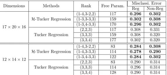
4.1 Performance comparison for the misclassification error of H-Tucker regression
and Tucker regression model on ADHD data. . . 65
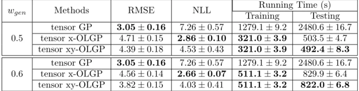
5.1 Computational complexity of tensor GP and tensor OLGP using product
prob-abilistic tensor kernel. . . 71 5.2 Performance comparison for the prediction of movement of shoulder marker
along x-axis on ECoG data, with data size=10 000. . . 72 5.3 Performance comparison for the prediction of movement of shoulder marker
along x-axis on ECoG data, with data size=36 000 and wgen= 0.4. . . 73
6.1 Performance comparison of IHOPLS, HOPLS and RNPLS for the averaged Q,
RMSEP and total learning time on UMPM data. . . 83 6.2 Performance comparison of IHOPLS, HOPLS and RNPLS for the averaged Q,
RMSEP and total learning time on ECoG data. . . 86
7.1 Performance comparison of NPLS, RNPLS, HOPLS, IHOPLS and RHOPLS for the averaged Q, RMSEP and learning time with I0 = 200 and b = 2 on
UMPM data. . . 103 7.2 Performance comparison of NPLS, RNPLS, HOPLS, IHOPLS and RHOPLS
for the averaged Q, RMSEP and learning time with I0 = 20% of the training
set and b = 2 on ECoG data. . . 107 7.3 Performance comparison of NPLS, RNPLS, HOPLS, IHOPLS and RHOPLS
for the averaged Q, RMSEP and learning time for L = [12, 16], K = [3, 10],
b = 2 on MHAD data. . . 109 7.4 Forecasting performance for lag = 3, trained with 50% of all the time series,
b = 1 on CCDS data. . . 110
8.1 Performance comparison of KMTPLS and MMCR for the optimal Rank, Q and
RMSEP on UMPM data. . . 118 8.2 Performance comparison of KMTPLS and MMCR for the averaged Q, RMSEP
Liste des figures
2.1 Illustration of a third-order tensor X ∈ RI1×I2×I3. . . . 9
2.2 Illustration of 1-mode fibers (left), 2-mode fibers (middle) and 3-mode fibers (right) of a third-order tensor. . . 10
2.3 Illustration of horizontal slices (left), vertical slices (middle) and frontal slices (right) of a third-order tensor. . . 11
2.4 Illustration of the matricization of a third-order tensor X ∈ RI1×I2×I3 in the first-mode (top) and second-mode (bottom). . . 13
2.5 Illustration of 2-mode tensor matrix multiplication Y = X ×2A. . . 15
2.6 Illustration of tensor vector multiplication in all the modes of a third-order tensor. 16 2.7 Illustration of rank-one third-order tensor X = a(1)◦ a(2)◦ a(3)∈ RI1×I2×I3. . . 17
2.8 Illustration of R-component CP decomposition of a third-order tensor. . . 18
2.9 Illustration of PARAFAC2 of a third-order tensor. . . 21
2.10 Illustration of Tucker decomposition of a third-order tensor. . . 22
2.11 Illustration of block component decomposition of a third-order tensor. . . 25
3.1 An illustration of high-order partial least squares (HOPLS) for M = 2 and L = 2. 33 3.2 An illustration of tensor regression layer (TRL). . . 48
4.1 Illustration of a balanced binary dimension tree T for a 5-order tensor. . . 54
4.2 Illustration of H-Tucker format for a 5-order tensor. . . 56
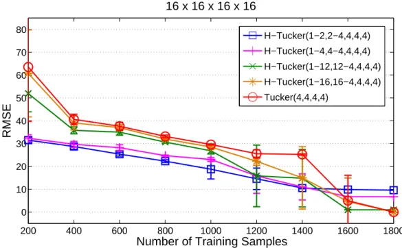
4.3 Performance comparison vs. number of samples for case of 4-order tensor. . . . 63
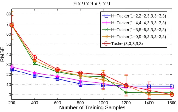
4.4 Performance comparison vs. number of samples for case of 5-order tensor. . . . 64
5.1 RMSE (top) and NLL (bottom) vs. number of training samples, wgen = 0.5, R = 6. . . 74
5.2 Learning time vs. number of training samples, wgen = 0.5, R = 6. . . 75
5.3 RMSE (top) and NLL (bottom) vs. number of local experts. . . 76
6.1 Prediction error (top) and CPU cost (bottom) of three methods over time, R = 8 and λ = 4 for IHOPLS and HOPLS for sequence length of 1050 and frequency at 5fps on UMPM. . . 84
6.2 Prediction error (top) and CPU cost (bottom) of three methods over time, R = 8 and λ = 4 for IHOPLS and HOPLS for sequence length of 5250 and frequency at 25fps on UMPM. . . 85
7.1 The RHOPLS scheme. The framework generates a set of initial factors for the initial data (Step 0 red arrow). At every iteration, the framework first generates a set of incremental factors for the new data (Step 1 yellow arrow). Then, the information contained in new data, represented in terms of factors, is added to current model by an appending operation (Step 2 blue arrow). Next, the augmented set of factors are truncated back into the ones with original sizes to yield new loadings (Step 3 purple arrow). The new individual core tensors are produced using an internal tensor representation of model (in terms of factors)
under the projection of the new loadings (Step 4 green arrow). . . 92
7.2 The initial approximation step of RHOPLS framework for t = 0. . . 93
7.3 The incremental approximation step of RHOPLS framework for t = 1. . . 94
7.4 The expansion step of RHOPLS framework for t = 1. . . 95
7.5 The compression step of RHOPLS framework for t = 1. . . 96
7.6 The projection step of RHOPLS framework for t = 1. . . 97
7.7 The whole RHOPLS scheme. . . 100
7.8 For “triangle” scenario, learning error and learning time versus the iteration. . . 101
7.9 For “table” scenario, learning error and learning time versus the iteration. . . . 102
7.10 The accuracy and learning time versus the number of latent vectors. . . 104
7.11 The accuracy and learning time versus the number of initial samples. . . 105
7.12 Performance versus sequence length (frequency). . . 106
7.13 An example of ground truth (150s time window) and the trajectories predicted by RHOPLS, HOPLS and RNPLS for Z-coordinate of the monkey’s hand. . . . 108
8.1 Illustration of the framework of kernel-based multiblock tensor partial least squares (KMTPLS) regression. . . 114
8.2 Performance comparison of KMTPLS and MMCR for the Q versus the different combination of cameras on UMPM data. . . 119
8.3 Performance comparison of KMTPLS for the Q when using the optimal rank versus the relative importance α on UMPM data. . . 120
8.4 Visualization of ground truth and the trajectories predicted by MMCR and KMTPLS in the “table” scenario. . . 121
8.5 Performance comparison of KMTPLS and MMCR for the best Q, RMSEP versus the number of input blocks on jumping action on MHAD data. . . 124
8.6 Performance comparison of KMTPLS and MMCR for the best Q, RMSEP versus the number of input blocks on bending action on MHAD data. . . 125
A.1 Illustration of the framework of partial least squares (PLS) regression. . . 132
Acknowledgements
I would like to express my sincerest gratitude to my supervisor, Prof. Brahim Chaib-draa, for his tremendous support to help me open the door of research world and guide me through the entire Ph.D study with his great advices. His insightful instructions always inspire me to open my mind and discover novel ideas ; his great patience and continuous encouragement are source of my strength to keep trying and never give up ; his professional attitudes and activities in research influence me a lot and will benefit me for my whole research career.
I owe my gratitude to Dr. Yali Wang, who helps me a lot with valuable suggestions and guidance at early stage of my research.
I am grateful to Dr. Qibin Zhao and Prof. Andrzej Cichocki from RIKEN brain science insti-tute, who provide me with a lot of precious advices and constructive comments.
I also thankful to Prof. Philippe Giguère, Prof. Claude-Guy Quimper and Prof. Jean-François Lalonde for their valuable guidance and wonderful courses, which expand my research horizons and help me lay solid foundations in research.
Finally, and most importantly, I dedicate this thesis to my great parents, my mom Jingyun Ma and my dad Jingbang Hou, who have always been there for me and supporting me with their deepest unconditional love.
Chapitre 1
Introduction
This chapter starts the thesis by introducing the context of our research and its motivations. Then, it gives the details about our contributions. Finally, it outlines the content of this thesis.
1.1
Context and Motivations for Tensor Regression
Regression is a statistical technique that attempts to study the relationship between two or more variables [Draper and Smith,2014;Chatterjee and Hadi,2015;Montgomery et al.,2015]. Specifically, regression analysis is able to predict one or more dependent variables (responses, outputs) from a set of independent variables (predictors, inputs), by exploring the correla-tions among these variables as well as explaining the factors behind the observed patterns. Regression is especially important because it can help you predict or analyze practically all types of data generated from complex systems in a large variety of applications. For instance, regression allows you to model property loss from fire as a function of a collection of variables such as degree of fire department involvement, response time and property value etc. If you find that response time is the key factor, you may need to build more fire stations. Extracting hidden structure and examining variables relationships, you may need to increase equipments or officers dispatched if you find that involvement variable is the key factor. Another example is that people may want to employ regression models to predict the amount of rainfall of next year based on the gauges from historical records.
The most commonly used regression models can typically be categorized, in terms of linearity, into linear regression and nonlinear regression. In particular, linear regression models describe relationship between dependent and independent variables using a linear function in parame-ters. Apart from simple regression model, linear regression models include multiple regression associated with multiple predictors, and multivariate regression corresponding to the case of linear regression model with multiple predictors and multiple responses. Normally, one may often encounter multivariate regression tasks where both the predictors and responses are arranged as vectors of variables or matrices of variables.
As an extension of ordinary linear regression models, the generalized linear model (GLM) [Nelder and Baker, 1972] is capable of modeling response variables via a particular distribu-tion other than normal distribudistribu-tion from the exponential family, which unifies logistic regres-sion [Hosmer and Lemeshow,2000], multinomial regression, Poisson regression [Cameron and Trivedi, 2013] and so on. Additionally, the class of partial least squares (PLS) [Wold et al.,
1984;Abdi,2010] models also belongs to the category of linear regression models.
Unlike linear regression modelings, nonlinear regression models characterizing nonlinear de-pendencies in data are generally assumed to be parametric, in which responses are modeled as a function of a combination of nonlinear parameters and predictors, where nonlinear parame-ters usually take the form of an exponential function, trigonometric function, power function, etc. Nonparametric nonlinear regression models frequently appear in the context of machine learning including Gaussian process (GP) [Rasmussen and Williams, 2005], artificial neural networks (ANN) [Haykin and Network, 2004], decision trees [Quinlan, 1986], support vector regression (SVR) [Smola and Vapnik,1997] and so on.
During the past few years, regular regression approaches, though being considered as mature techniques, have confronted new great challenges posed by numerous real-world regression tasks whose predictors and (or) responses take the form of high-order high-dimensional ar-rays with complex structures, also known as tensors [Kolda and Bader,2009;Cichocki et al.,
2009; Acar and Yener, 2009; Cichocki, 2013; Cichocki et al., 2015; Cong et al., 2015]. With the advancement of modern technologies, such high-order tensors (multiway arrays) are quite widespread and abound in a broad range of applications, including analytical chemistry [ An-dersen and Bro,2003;Bro,2006], computational neuroscience [Miwakeichi et al.,2004; Ander-sen and Rayens,2004], computer vision [Vasilescu and Terzopoulos, 2002;Wang and Ahuja,
2008], industrial process control [Luo et al.,2015], data mining [Acar et al.,2005;Kolda et al.,
2005] and so on.
For instance, wavelet-transformed multichannel electroencephalogram (EEG) data can be or-ganized as a third-order tensor with modes time × frequency × channels [Miwakeichi et al.,
2004; Cichocki, 2013; Cichocki et al., 2015; Cong et al., 2015] ; fluorescence spectroscopic data can be arranged as a third-order tensor with modes samples × excitation wavelengths × emission wavelengths [Andersen and Bro,2003] ; video sequences can naturally be modeled as third-order tensor with modes x-coordinates × y-coordinates × frames [Wang and Ahuja,
2008] and face images with various conditions can be represented as a fifth-order tensor having modes pixels × illuminations × expressions × viewpoints × identities [Vasilescu and Terzopou-los,2002]. In addition, the related tensor data analysis (multiway data analysis) [Kolda and Bader,2009;Acar and Yener,2009] approaches and tools have also been studied extensively in a variety of fields, with the fundamental goals of exploring the correlations among variables as well as discovering the underlying hidden patterns so as to find a a summarization of tensor data.
The primary reason why regular regression methods fail to appropriately handle high-order tensors is due to the fact that those data contain multiway structural information (i.e., the information about the patterns of correlations among different modalities in high-order ten-sors) which cannot be directly captured by the conventional vector-based or matrix-based regression models. For instance, in the application of brain imaging data analysis, we aim to establish the associations between the magnetic resonance imaging (MRI) brain images and the clinical outcomes. This problem can be formulated as a regression task with predictor variable taking the form of 3-order tensor and with response variable being the scalar clinical outcome, predicting whether the subject is healthy or not.
In order to address the high-order input, it is a common practice to apply classical regression techniques to tensorial brain images by first transforming them into vectors (matrices) via some vectorization (unfolding) operations and then feeding them to classical models. Nevertheless, there are two significant challenges as a consequence of this procedure. Firstly, the ultrahigh dimensionality of tensorial input like 3D or 4D brain images results in a huge amount of pa-rameters, which undoubtedly leads to an overfitting situation as well as breaks the theoretical guarantees of classical regression approaches. Secondly, using such operations of vectorizing (or unfolding) as proposed will inevitably destroy underlying multiway structure contained in tensorial input and lose intrinsic correlations among the pixels, causing substantial information loss during the regression.
In addition to above issues, the classical regression models based on the matrix analysis ap-proaches have also been shown to be inferior in terms of difficulty of interpretation, sensitivity to noise as well as absence of uniqueness [Acar and Yener,2009]. Let us take the analysis of third-order multichannel EEG data as an example. If we unfold the predictor in the channels mode (i.e., resultant matrix with mode channels × time-frequency) and employ matrix-based regression model (i.e., unfolded PLS regression [Abdi,2010], see Appendix A.1), then the set of factors (signatures, patterns) extracted from the time-frequency mode become very hard to interpret, leading to the difficulties in understanding the brain activities associated with those two factors (signatures, patterns).
1.2
Tensor-based Regression Models and Their Applications
Motivated by the extensive applicability of tensor data and the limitations of classical re-gression models, we propose to investigate in this thesis the tensor based rere-gression models and their applications. More specifically, we aim to develop a novel class of regression models dealing with high-order tensorial predictors and (or) high-order tensorial responses and apply them in various real-life applications. The work is accomplished by making use of multiway fac-tor modelings (i.e., canonical decomposition/parallel facfac-tor analysis (CP) model [Carroll and Chang, 1970;Harshman, 1970] or Tucker model [Tucker,1963;De Lathauwer et al., 2000a])
and their related tensor (multiway) analysis approaches [Kolda and Bader, 2009; Cichocki et al.,2009;Acar and Yener,2009]. In general, these models and analysis approaches are more beneficial over their matrix-based counterparts since they are designed to naturally repre-sent and preserve the multiway nature of the tensorial data. Therefore, by combing multiway modeling ideas with classical regression models, we provided efficient tensor-variate regression models which are able to effectively capture the underlying inherent structural information in tensors, resulting in significantly improved predictability.
If we now model the previous MRI images using R-component CP model instead of explicit long vector, then the number of parameters will be drastically reduced from O(ID) to O(DIR), where D is tensor order while I stands for the maximum size in each mode and R I. In this case, not only the correlations among pixels are preserved, but also the CP-based model is in fact statistically simpler, which is not prone to overfitting for the case of MRI application where the number of observations is rather limited.
Once again, referring back to the previous EEG example, if we apply multiway PLS model [Bro,1996] to third-order EEG array, we are able to extract a set of factors that individually accounts for the temporal pattern of brain activities from time mode as well as the spectral pattern of brain activities associated with frequency mode, respectively. The latent scores, extracted from channels mode, can easily be interpreted as the coefficients of the combination of different brain activity patterns, which are used to measure their relative contributions. Such advantage in the ease of interpretation can further result in the property of robustness to noise since the number of components in model can be reasonably specified according to the scientific assumption and experimental results.
Thus, tensor-variate regression, as we can see, is free of the above discussed limitations of conventional regression methods and is expected as a promising research direction. In this thesis, we investigate and extend several tensor-variate modeling strategies from different per-spectives, including the aspect of multilinear model with potentially much higher-order tensor input, the aspect of nonlinear online model with scalar output, the aspect of multilinear online model with general tensor input and tensor output. We also investigate the aspect of model merging tensor blocks from different sources for boosting the predictive power. Furthermore, our proposed tensor-variate regression models and algorithms have been validated on a num-ber of real-world representative applications from different disciplines such as the prediction of brain disease from medical MRI images in computational neuroscience, the reconstruction of limb trajectories from monkey’s brain signals in neural signal processing, the estimation of human pose positions from video sequences in computer vision, etc.
In the following sections, we summarize our contributions and describe the outline of this thesis.
1.3
Main Contributions
1.3.1 Hierarchical Tucker Tensor Regression : Application to Brain Imaging Data Analysis
In [Hou and Chaib-draa,2015], we present a novel generalized linear tensor regression model, which takes tensor-variate inputs as predictors and finds low-rank almost best approximation of regression coefficient arrays using hierarchical Tucker decomposition. With limited sample size, our model is highly compact and very efficient as it requires only O(DR3+ DIR) parameters for order D tensors of mode size I and rank R. Thus, it avoids the exponential growth in D, in contrast to O(RD+ DIR) parameters of Tucker regression modeling. Our model also maintains the flexibility like classical Tucker regression by allowing distinct ranks on different modes according to a dimension tree structure. We validated our new model on synthetic data, and we also applied it to real-life MRI images to show its effectiveness in predicting the human brain disease of attention deficit hyperactivity disorder.
1.3.2 Online Local Gaussian Process for Tensor-Variate Regression : Application to Fast Reconstruction of Limb Movement from Brain Signal
In [Hou et al.,2015], we overcome the computational issues of existing tensor Gaussian process (tensor GP) regression approaches for large data sets by introducing a computationally-efficient tensor-variate regression approach in which the latent function is flexibly modeled by using online local Gaussian process (OLGP). By doing so, the large data set is efficiently processed by constructing a number of small-sized GP experts in an online fashion. Furthermore, we introduce two searching strategies to find local GP experts to make accurate predictions with a Gaussian mixture representation. Finally, we apply our approach to a real-life regression task, reconstruction of limb movements from brain signal, to show its effectiveness and scalability for large data sets.
1.3.3 Online Incremental Higher-order Partial Least Squares Regression for Fast Reconstruction of Motion Trajectories from Tensor Streams The higher-order partial least squares (HOPLS) is considered as the state-of-the-art tensor-variate regression modeling for predicting a tensor response from a tensor input. However, the standard HOPLS can quickly become computationally prohibitive or merely intractable, espe-cially when huge and time-evolving tensorial streams arrive over time in dynamic application environments. In [Hou and Chaib-draa, 2016], we present a computationally efficient online tensor regression algorithm, namely incremental higher-order partial least squares (IHOPLS), for adapting HOPLS to the setting of infinite time-dependent tensor streams. By incrementally clustering the projected latent variables in latent space and summarizing the previous data,
IHOPLS is able to recursively update the projection matrices and core tensors over time, re-sulting in greatly reduced costs in terms of both memory and running time while maintaining high prediction accuracy. For the experiments, we apply IHOPLS to two real-life applications, i.e., reconstruction of 3D motion trajectories from videos and ECoG streaming signals.
1.3.4 Fast Recursive Tensor Sequential Learning for Regression
In this specific work, we develop a super-fast sequential tensor regression framework, namely recursive higher-order partial least squares (RHOPLS) [Hou and Chaib-draa, 2017]. It ad-dresses the great challenges posed by the limited storage space and fast processing time al-lowed by dynamic environments when dealing with very large-scale high-speed general tensor sequences. Smartly integrating a low-rank modification strategy of the Tucker into partial least squares (PLS), we efficiently update the PLS-based regression coefficients by effectively merging the new data into the previous low-rank approximation of the model at a small-scale factor (feature) level instead of the large raw data (observation) level. Unlike batch approaches, which require accessing the entire data, RHOPLS conducts a blockwise consecutive calculation scheme and thus it stores only a small set of factors. Our approach is orders of magnitude faster than all other methods while maintaining a highly comparable predictability with the cutting-edge batch methods, as verified on challenging real-life tasks.
1.3.5 Common and Discriminative Subspace Kernel-based Multiblock Tensor Partial Least Squares Regression
In [Hou et al., 2016], we introduce a new generalized nonlinear tensor regression framework called kernel-based multiblock tensor partial least squares (KMTPLS). With this framework, we can predict a set of dependent tensor blocks from a set of independent tensor blocks through the extraction of a small number of common and discriminative latent components. By con-sidering both common and discriminative features, KMTPLS effectively fuses the information from multiple tensorial data sources and unifies the single and multiblock tensor regression scenarios into one general model. Moreover, in contrast to multilinear model, KMTPLS suc-cessfully addresses the nonlinear dependencies between multiple responses and predictor tensor blocks by combining kernel machines with joint Tucker decomposition, resulting in a signifi-cant performance gain in terms of predictability. An efficient learning algorithm for KMTPLS based on sequentially extracting common and discriminative latent vectors is also presented. Finally, as for the applications, we employ KMTPLS on a regression task in computer vision, i.e., reconstruction of human pose from multiview video sequences.
1.4
Thesis Outline
This thesis is organized as follows. Chapter 2 gives an overview of the basic tensor defini-tions, its associated operations and the most commonly used tensor decomposition tools and
their extensions. Chapter 3 summarizes the concepts of tensor regression models and the re-cent advances in the work related to what we are proposing. The hierarchical Tucker tensor regression model is presented in Chapter 4. Chapter 5 introduces the nonlinear online local Gaussian process for regression task with tensor input and scalar output. Another two online tensor regression models based on PLS framework are introduced in Chapter 6 and 7, with the goal of addressing the problem of speed and storage complexity when dealing with general tensor input and tensor output. Chapter 8 proposes a generalized nonlinear tensor regression framework, as an effective tool of integrating tensorial data from different sources, for predict-ing a set of dependent tensor blocks from a set of independent tensor blocks. Finally, Chapter 9 concludes the thesis and discuss some future research directions.
Chapitre 2
Tensor Preliminaries
This chapter reviews several fundamental parts about tensor that are necessary for understand-ing tensor-variate regression in the remainunderstand-ing chapters. It begins by introducunderstand-ing some notations of tensor and some basic definitions of tensor algebra. Then it presents the key concept of ten-sor decomposition (factorization), also known as multiway models or multilinear models. This concept turns out to be an extremely useful tool to decompose a high-order tensor object into a collection of factors in low-dimensional subspace. Subsequently, it introduces several extended variants of tensor decomposition that are very useful for the regression problems as studied in this thesis. Finally, it gives a high-level overview of various strategies for scaling up tensor decompositions.
2.1
Tensor Basics
2.1.1 Tensor Definitions and Notations
Tensors [Kolda and Bader,2009; Cichocki et al.,2009; Cichocki,2013;Cichocki et al.,2015;
Cong et al.,2015] are higher-order generalizations of vectors and matrices. They also refer to as multiway arrays of real numbers. Throughout the thesis, higher-order tensors will be denoted as X ∈ RI1×I2×···×ID in calligraphy letters, where D is the order of X . Matrices represented
by boldface capital letters X ∈ RI1×I2 are tensors of order two, while the vectors denote
first-order tensors and are represented by boldface low-case letters x ∈ RI1. Here, the order
D represents the number of dimensions and each dimension d ∈ D of tensor is called mode or way [Tucker, 1963,1964]. The number of variables Id in the mode d is used to represent the
dimensionality of that mode. In other words, D-order tensor X ∈ RI1×I2×···×ID has D modes
(ways) with dimensionality Id in the mode d, where d = 1, ..., D. The ith entry of a vector x
is denoted by xi and the (i, j) entry of a matrix X is denoted by xi,j. Likewise, we denote the entry (i1, i2, ..., iD) of D-order tensor X ∈ RI1×I2×···×ID as xi1,i2,...,iD. An example of a third
order tensor with three modes is illustrated in Figure 2.1.
Figure 2.2 – Illustration of 1-mode fibers (left), 2-mode fibers (middle) and 3-mode fibers (right) of a third-order tensor.
The d-mode vector of tensor X , also known as d-mode fiber, is an element of RId, which is
obtained by varying the index Id while keeping other indices fixed. For instance, for a third order tensor, a fiber x:,4,3from 1-mode fibers (columns), a fiber x5,:,1 from 2-mode fibers (rows) and a fiber x2,4,: from 3-mode fibers (tubes) are shown in highlighted color in Figure 2.2,
respectively. Here we use “ : ” to denote free indices that range over a specific mode.
Similarly, if we vary two indices by fixing the other one index in a third order tensor, then we will get a slice (slab), i.e., a horizontal slice x3,:,:, a vertical slice x:,4,: and a frontal slice x:,:,1
are shown in highlighted color in Figure 2.3.
Figure 2.3 – Illustration of horizontal slices (left), vertical slices (middle) and frontal slices (right) of a third-order tensor.
2.1.2 Relevant Matrix Algebra
The Kronecker product [Smilde et al.,2005] between matrix X ∈ RI×J and matrix Y ∈ RK×L
yielding a block matrix of size IK × J L is denoted by symbol ⊗ as
X ⊗ Y = x11Y x12Y · · · x1jY x21Y x22Y · · · x2jY · · · · xi1Y xi2Y · · · xijY ∈ RIK×J L, (2.1)
and X ⊗ Y can also be expressed in form of columnwise Kronecker product as
X ⊗ Y = [x1⊗ y1, x1⊗ y2, x1⊗ y3, ..., xJ⊗ yL−1, xJ⊗ yL] ∈ RIK×J L
= [vec(y1xT1), vec(y2xT1), vec(y3xT1), ..., vec(yL−1xTJ), vec(yLxTJ)],
(2.2)
where vec represents the vectorization operation.
The mixed-product property of Kronecker product, which will be found useful in this thesis, states that if X, Y, A and B are conformable matrices whose dimensions are suitable for multiplications such that the matrix product XY and AB can be formed, then we have
(X ⊗ A)(Y ⊗ B) = XY ⊗ AB. (2.3)
The Khatri-Rao product [Smilde et al., 2005] between matrix X = [x1, ..., xJ] ∈ RI×J and
Y = [y1, ..., yJ] ∈ RK×J having the equal number of columns is defined using columnwise Kronecker product of matrices as
The Hadamard product [Smilde et al.,2005] between matrix X ∈ RI×J and matrix Y ∈ RI×J
with equal matrix size is the entrywise product denoted by symbol ∗
X ∗ Y = x11y11 x12y12 · · · x1jy1j x21y21 x22y22 · · · x2jy2j · · · · xi1yi1 xi2yi2 · · · xijyij ∈ RI×J. (2.5) 2.1.3 Tensor Matricization
For high-order tensors, it is usually beneficial to be represented using vectors or matrices so that the powerful matrix analysis techniques can readily be applied to the lower subspaces.
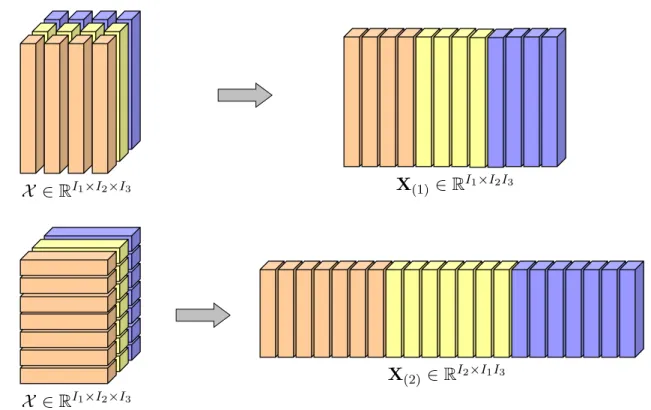
The d-mode matricization (unfolding, flattening) of a tensor X ∈ RI1×I2×···×ID [Kiers,2000;
De Lathauwer et al.,2000a], defined as X(d) ∈ RId×I1···Id−1Id+1···ID, is the process of rearranging
the d-mode vectors (fibers) into the columns of the resulting matrix. In other words, according to a prespecified order, we collect all d-mode vectors of a tensor and then concatenate them side by side, leading to a matrix with size Id× I1· · · Id−1Id+1· · · ID.
Mathematically, the mapping from an entry (i1, i2, ..., iD) of a tensor X ∈ RI1×I2×···×ID to an
entry (id, j) of the unfolded matrix can be established by
j = 1 + D X t6=d (it− 1)Jt with Jt= t−1 Y p6=t ip. (2.6)
Figure 2.4 demonstrates the examples where a third order tensor X ∈ RI1×I2×I3 is unfolded
in the first-mode and second-mode, resulting in a matrix X(1) of size I1× I2I3 and a matrix
X(2) of size I2× I1I3, respectively.
The vectorization of a tensor X ∈ RI1×I2×···×ID is defined as
vec(X ) = vec(X(1)), (2.7)
that is, the vectorization of the corresponding first-mode unfolded matrix X(1).
Specifically, the vectorization of a matrix X ∈ RI×J is obtained by stacking the matrix columns {xj}Jj=1 into a long vector x ∈ RIJ
x = vec(X) = x1 x2 ... xJ ∈ RIJ. (2.8)
Two important properties associated with the matrix vectorization operator are
vec(X)Tvec(Y) = trace(XTY) (2.9)
Figure 2.4 – Illustration of the matricization of a third-order tensor X ∈ RI1×I2×I3 in the
first-mode (top) and second-mode (bottom).
and
vec(XYZ) = (ZT⊗ X) vec(Y), (2.10)
where ⊗ stands for the standard Kronecker product.
2.1.4 Tensor Multiplication
The outer product of tensor X ∈ RJ1×···×JP and tensor Y ∈ RK1×···×KQ, which produces a
tensor of size J1× · · · × JP × K1× · · · × KQ, is denoted as
Z = X ◦ Y (2.11)
with each entry satisfying
zj1,...,jP,k1,...,kQ= xj1,...,jPyk1,...,kQ. (2.12)
The inner product between two tensors X , Y ∈ RI1×···×ID having the same order and equal
size is given by
z = hX , Yi = hvec(X ), vec(Y)i, (2.13) where z ∈ R is a scalar. In entrywise form, we have
z = hX , Yi = I1 X i1=1 I2 X i2=1 · · · ID X iD=1 xi1,...,iDyi1,...,iD. (2.14)
Having defined the tensor inner product, the Frobenius norm of tensor X ∈ RI1×I2×···×ID
follows the definition as
kX kF =phX , X i. (2.15)
The contracted product between X ∈ RI1×···×IC×J1×···×JP and Y ∈ RI1×···×IC×K1×···×KQ with
equal size along the first C modes yields a tensor Z ∈ RJ1×···×JP×K1×···×KQ in the following
element expression zj1,...,jP,k1,...,kQ = hX , Yi1,...,C;1,...,C(j1, ..., jP, k1, ..., kQ) = I1 X i1=1 · · · IC X iC=1 xi1,...,iC,j1,...,jPyi1,...,iC,k1,...,kQ, (2.16)
which means the entries in the resulting tensor are obtained by summing out the product of each corresponding entry pair along the first few common indices between two tensor multi-pliers.
On one hand, it is a simple matter to see that the tensor inner product is actually a special case of the tensor contracted product when all the modes are in common between two tensor multipliers, e.g., X ∈ RI1×···×IC and Y ∈ RI1×···×IC
z = hX , Yi = hX , Yi1,...,C;1,...,C. (2.17)
On the other hand, with no common indices between two tensors, the tensor contracted product turns out to be the tensor outer product as introduced in (2.11)
Z = X ◦ Y = hX , Yi0;0. (2.18)
The tensor-matrix multiplication is generalized from standard matrix multiplication via ma-trix matricization. Specifically, when a tensor X ∈ RI1×I2×···×ID is multiplied by a
ma-trix A ∈ RJd×Id, it is first unfolded in the dth mode to obtain X
(d), then the matrix
product Y = AX(d) is computed. Finally, the resulting Y is reshaped back to a tensor Y ∈ RI1×···×Id−1×Jd×Id+1×···×ID. This operation is depicted in Figure 2.5 for the case of 2-mode
tensor matrix multiplication of a third order tensor. We refer such tensor-matrix multiplication as the d-mode tensor matrix product of tensor X ∈ RI1×I2×···×ID and matrix A ∈ RJd×Id
Y = X ×dA ∈ RI1×···×Id−1×Jd×Id+1×···×ID, (2.19)
which can also be expressed in an elementwise form
yi1,...,id−1,jd,id+1,...,iD = Id X id=1 yi1,...,id,...,iDajd,id. (2.20) 14
Figure 2.5 – Illustration of 2-mode tensor matrix multiplication Y = X ×2A.
Assuming the conforming dimensions among the matrices and tensors, one can easily verify the following properties :
hX ×dA, Yi = hX , Y ×dATi, (X ×cA) ×dB = (X ×dB) ×cA, c 6= d, (X ×dA) ×dB = X ×dBA, (2.21) and (X ×1A(1)· · · ×DA(D))(d) = A(d)X(d)(A(D)⊗ · · · ⊗ A(d+1)⊗ A(d−1)⊗ · · · ⊗ A(1))T. (2.22)
Similarly, d-mode tensor vector product between a tensor X ∈ RI1×I2×···×ID and a vector
a ∈ RId is defined as
Y = X ¯×da ∈ RI1×···×Id−1×Id+1×···×ID. (2.23)
In element form, we get
yi1,...,id−1,id+1,...,iD =
Id
X
id=1
yi1,...,id,...,iDaid. (2.24)
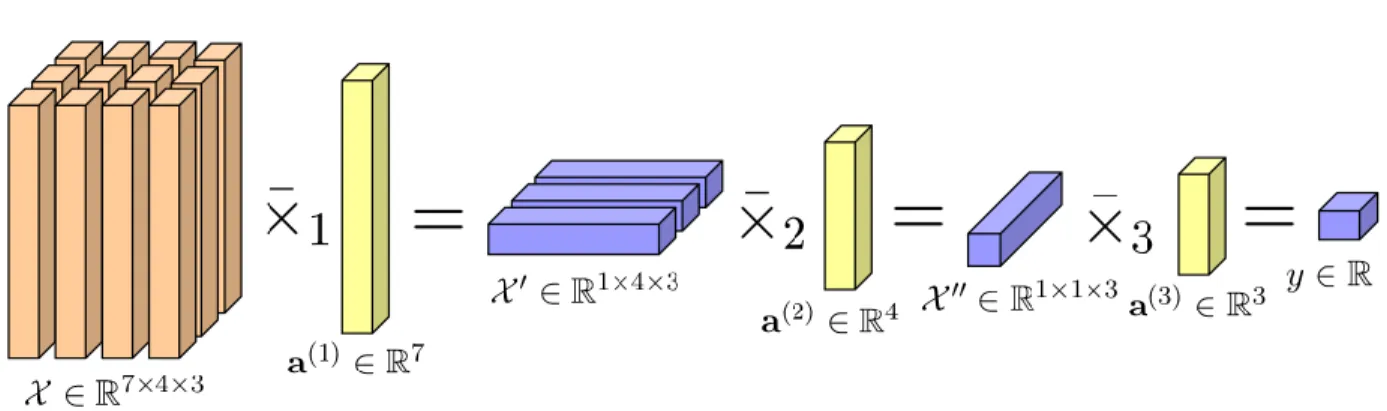
If we multiply tensor X ∈ RI1×I2×···×ID by a set of vectors {a ∈ RId}D
d=1, each of which is
associated with one specific mode d, then the result is a scalar formulated by
y = X ¯×1a(1)ׯ2 · · · ¯×Da(D)∈ R. (2.25) An example of tensor vector multiplication of a third order tensor is illustrated in Figure 2.6, in which a third order tensor X ∈ R7×4×3is sequentially multiplied by vectors a1 ∈ R7, a2 ∈ R4
and a3 ∈ R3 along the mode 1, 2 and 3, respectively, ending up with a scalar y ∈ R.
When satisfying the relative ordering between the modes, the commutative property also holds for tensor vector product as below
Figure 2.6 – Illustration of tensor vector multiplication in all the modes of a third-order tensor.
2.1.5 Tensor Rank
The d-rank of a tensor X ∈ RI1×I2×···×ID, denoted as rank
d(X ), is the column rank of the
unfolding matrix X(d). In other words, it is the dimension of the vector space spanned by d-mode vectors. In the context of d-mode matricization, we can establish that
rankd(X ) = rank(X(d)). (2.27)
A tensor X for which rd = rankd(X ) for d = 1, ..., D is called a rank-(r1, r2, ..., rD) tensor,
and the D-tuple (r1, r2, ..., rD) is defined as the multilinear rank of X .
In addition to multilinear rank, an alternative notion of rank named tensor rank exists and it is built on the basis of rank-one tensor. The D-order tensor X is rank-one tensor if it consists of the outer product of D vectors {a(d) ∈ RId}D
d=1
X = a(1)◦ a(2)◦ · · · ◦ a(D), (2.28)
where ◦ is the vector outer product introduced in (2.11). Writing this in an equivalent entry expression, it gives xi1,i2,...,iD = a (1) i1 a (2) i2 · · · a (D) iD . (2.29)
An example of rank-one third-order tensor is shown in Figure 2.7, where it factorizes as the outer product of three vectors a(1), a(2) and a(3) from three modes.
The tensor rank, namely rank(X ), is defined to be the minimum number of the sum of rank-one tensor that can exactly factorize tensor X
rank(X ) := arg min{R ∈ N : X =
R
X
r=1
a(1)r ◦ a(2)r ◦ · · · ◦ a(D)r }. (2.30)
Particularly, for matrices (second-order tensors), the following equation holds
rank1(X ) = rank2(X ) = rank(X ). (2.31)
Figure 2.7 – Illustration of rank-one third-order tensor X = a(1)◦ a(2)◦ a(3)∈ RI1×I2×I3.
2.2
Tensor Decompositions
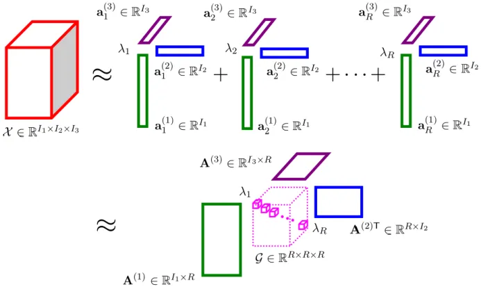
The strength of tensor modelings lies in its associated decomposition tools that are capable of representing high-order data in terms of low-dimensional factors. The concept of tensor decomposition (factorization) was originally introduced byHitchcock[1927,1928]. Nowadays, higher-order tensor decompositions (factorizations) are frequently applied in a variety of fields such as chemometrics, neuroscience, image/video analysis and signal processing. Most of ex-isting decomposition models can trace back to two fundamental decomposition formats, that are canonical decomposition/parallel factor analysis (or CANDECOMP/PARAFAC, or sim-ply CP) [Carroll and Chang,1970; Harshman, 1970;Kiers, 2000] decomposition and Tucker [Tucker,1963;De Lathauwer et al.,2000a] decomposition.
2.2.1 CP decomposition
The CP decomposition [Carroll and Chang,1970;Harshman,1970;Kiers,2000] initially intro-duced as the polyadic form [Hitchcock,1927] of a tensor generalizes the bilinear factor models to multilinear data. Mathematically, the R-component CP model boils down to factorizing a tensor X ∈ RI1×I2×···×ID as a linear combination of rank-one tensors as
X =
R
X
r=1
λra(1)r ◦ a(2)r ◦ · · · ◦ a(D)r + ε (2.32)
or in equivalent elementwise form
xi1,i2,...,iD = R X r=1 λra(1)i1,ra (2) i2,r· · · a (D) iD,r+ εi1,i2,...,iD, (2.33)
where the symbol ◦ is the outer product operator. The normalized unit vector a(d)r for r =
1, ..., R indicates the rth column of factor matrix A(d) = [a(d)1 , a(d)2 , ..., a(d)R ] ∈ RId×R from
and R is the tensor rank. ε is the residual with same size as tensor X . For instance, the top part of Figure 2.8 demonstrates a R-component CP decomposition of a three-way array, where a(1)r , a(2)r and a(3)r correspond to the factors associated with rth sub-tensor component
extracted from the corresponding modes, respectively.
Figure 2.8 – Illustration of R-component CP decomposition of a third-order tensor.
The CP in equation (2.32) can also be converted into a more compact matrix form in terms of d-mode unfolding matrix X(d) using Khatri-Rao product defined in (2.4)
X(d)= A(d)Λ(A(D) · · · A(d+1) A(d−1) · · · A(1))T+ E, (2.34)
where diagonal matrix Λ = diag(λ1, λ2, ..., λR) and E represents the residual. Applying
vec-torization property (2.10) to matrix form (2.34), we reach the vectorized form of CP as
vec(X ) = (A(D) · · · A(1)) vec(Λ) + vec(ε). (2.35)
For the special case of third-order tensor, (2.32) can be rewritten in a alternative matrix form as
Xi = A(1)DiA(2)T+ Ei for i = 1, ..., I3, (2.36)
where Xi corresponds to the ith frontal slice of a third-order tensor X . Di = diag(a(3)i,: ) is a
diagonal matrix with diagonal elements from the ith row of third mode factor matrix A(3). Ei is the error associated with the ith frontal slice. Note that here in (2.36) the factor matrices {A(d)}3
d=1 are not normalized.
For the simplicity of notation, the CP model can be expressed in a succinct way [Kolda and Bader,2009] as
X ≈ [Λ, A(1), A(2), ..., A(D)]. (2.37)
One favorable property about CP model is that, under certain mild conditions [Kruskal,1989], one is able to obtain a unique CP factorization up to permutation indeterminacy and scaling indeterminacy. In other words, the CP model can be uniquely identified except that columns of factor matrices, i.e., A(d) = [a(d)1 , a(d)2 , ..., a(d)R ] with d = 1, ..., D, can be arbitrarily reordered. It can be scaled as long as product of scaling coefficients of columns remains constant.
Nevertheless, such benefit is achieved at the cost of strict constraints imposed on the CP model, whose factors in distinct modes can only interact factorwise with each other. In other words, CP model is inadequate in terms of degrees of freedom. For example in Figure 2.8, the factor a(1)r in the first mode is required to communicate merely with the factor a(2)r in the
second mode and the factor a(3)r in the third mode, leading to the same number of factors
for all modes. Another disadvantage is that a CP approximation may be ill-posed and may produce unstable estimation of its components [Cichocki et al.,2009].
As a generalization of singular value decomposition (SVD) (see Appendix A.3) to high-order tensor, CP factorizes a tensor as a sum of rank-one tensors, which is analogous to SVD in the sense that SVD decomposes a matrix into a sum of rank-one matrices. Nevertheless, unlike SVD, the orthogonality of CP on factor matrices can hardly be satisfied.
It is worth noting that CP decomposition only demands the storage of O(DIR) entries in contrast to that of O(ID) for I = max{Id}Dd=1, which become very attractive when R I.
The classical algorithms for computing CP model [Carroll and Chang,1970;Harshman,1970] are based on the alternating least squares (ALS) style algorithm [Kroonenberg and De Leeuw,
1980] that estimates one factor matrix at a time by keeping the rest factor matrices fixed. Mathematically, the objective is to minimize the approximation error by iteratively solving the following least square problem, with respect to one specific factor matrix A(d) at a time
min kX − ¯X k = min kX(d)− A(d)(A(D) · · · A(d+1) A(d−1) · · · A(1))Tk, (2.38)
where refers to the Khatri-Rao operator. Thus, the solution of (2.38) regarding the d-mode factor matrix A(d) can easily be computed as
A(d)= X(d)[(A(D) · · · A(d+1) A(d−1) · · · A(1))T]† (2.39)
with † being as the pseudo inverse. Following the similar pattern, the algorithm alternately updates factor matrices for all d = 1..., D modes and stops when a certain convergence cri-terion is met. Though as a simple and practical solution for computing CP, the ALS-based algorithm does not guarantee a global optimum due to the non-convex property of (2.38).
Additionally, ALS-based algorithm has a slow convergence rate [Cichocki et al., 2009]. The CP-ALS procedure is summarized in Algorithm 1, in which equation (2.39) corresponds to line 6 and 7.
Algorithm 1 CP-ALS [Carroll and Chang,1970;Harshman,1970] 1: Input : D-order tensor X ∈ RI1×I2×···×ID, tensor rank R
2: Output : coefficients {λd}D
d=1, factor matrices {A(d)∈ RId ×R}D
d=1
3: Initialize : randomly initialize {A(d)}D d=1 4: repeat 5: for d = 1, ..., D do 6: Td← A(1)TA(1)∗ · · · ∗ A(d−1)TA(d−1)∗ A(d+1)TA(d+1)∗ · · · ∗ A(D)TA(D) 7: A(d) ← X(d)(A(D) · · · A(d+1) A(d−1) · · · A(1))T† d 8: end for
9: until the convergence criterion is satisfied
One notable extension of standard CP model is referred to as PARAFAC2 [Harshman,1972]. It was introduced to model third-order tensors with frontal slices having different dimensionality in one mode. For example, the data from industrial batch process control, e.g., time duration × variables × batches, usually varies in time duration mode due to the unavoidable disturbances and changes of operating conditions, leading to batch data with uneven-length frontal slices. In fact, PARAFAC2 simultaneously decomposes a collection of matrices with each having equal number of columns but different row size. Unlike CP model that applies the same factors across all frontal slices (e.g., A(1) and A(2) linked with Xi for i = 1, ..., I3 in (2.36)), PARAFAC2
relaxes CP to allow for distinct factors associated with different frontal slices in the first mode. More formally, PARAFAC2 model can be derived from formulation (2.36) by enforcing additional constraint on factor matrix in the first mode as
Xi = A(1)i DiA(2)T+ Ei
s.t A(1)Ti A(1)i = α for i = 1, ..., I3,
(2.40)
where the 1-mode factor matrix A(1)i corresponds to ith frontal slice. α is a constant. The constraint imposed on A(1)i indicates that the matrix product of A(1)i with its transpose is invariant for all frontal slices {Xi}Ii=13 of a third order tensor X ∈ RI1×I2×I3. Such constraint is
introduced for the purpose of inducing the uniqueness properties of PARAFAC2 [Harshman,
1972]. Figure 2.9 shows an example of PARAFAC2 decomposition of an irregular third-order tensor having 4 frontal slices with different 1-mode sizes.
Another well-known extension of CP model called shifted PARAFAC (s-PARAFAC) is pro-posed byHarshman et al.[2003] with the aim to handle the shifting factors in sequential data, e.g., time series or spectral data. Compared to ordinary CP format, s-PARAFAC is relaxed to allow the factor matrix, in one mode of a third-order tensor, to be shifted by certain amount
Figure 2.9 – Illustration of PARAFAC2 of a third-order tensor.
of positions. Concretely, s-PARAFAC for mode 2 looks something like
Xi= A(1)DiSsi(A
(2))T+ E
i for i = 1, ..., I3, (2.41)
where almost all the notations are identical to that of (2.36) except that shift function Ssi shifts all the columns of factor matrix A(2) by some amount according to vector si∈ RR. The
R elements in vector si are specified the ith row of shift matrix S ∈ RI3×R.
Generalizing convolutive nonnegative matrix factorization (CNMF) [Smaragdis,2004] to high-order tensor, convolutive PARAFAC (c-PARAFAC) [Mørup and Schmidt,2006] was proposed to model convolutive mixtures of multichannel time-frequency spectral data. Mathematically, the matrix representation is formulated in terms of frontal slice Xi as
Xi= A(1)
Θ−1
X
θ=0
D(θ+1)i (S↑(θ)A(2))T+ Ei for i = 1, ..., I3, (2.42)
where D(θ)i is a diagonal matrix whose entries are taken from the ith row of the θth factor matrix Aθin a set of factor matrices {A(3)θ }Θ
θ=1associated with the third mode. S↑(θ)is denoted
as vertical shift operator that enables us to shift matrix θ rows in the up direction, leaving the new rows shifted into the matrix from the bottom being zero.
2.2.2 Tucker decomposition
Another tensor decomposition in widespread use is called Tucker decomposition [Tucker,1963;
De Lathauwer et al., 2000a], which was introduced by relaxing the constraint in CP model to allow the arbitrary interaction of factors among different modes. The standard Tucker decomposition can be viewed as order principal component analysis. It converts high-order array X into a core tensor G that is transformed by an orthogonal factor matrix A(d) along each mode d in the following way
or equivalently in the outer product representation X = R1 X j1=1 R2 X j2=1 · · · RD X jd=1 gi1,i2,...,iDaj1◦ aj2 ◦ · · · ◦ ajD + ε (2.44)
or in an equivalent scalar representation
xi1,i2,...,iD = R1 X j1=1 R2 X j2=1 · · · RD X jd=1 gi1,i2,...,iDai1,j1ai2,j2· · · aiD,jD+ εi1,i2,...,iD, (2.45)
where A(d) ∈ RId×Rd is the factor matrix. R
d serves as the d-rank of X in mode d. G ∈
RR1×R2×···×RDrepresents the core tensor indicating the interaction level among factor matrices from different modes. Thus, this core tensor G provides us with a much better way to capture the underlying multiway structure of tensor data. ε reflects the residuals.
A Tucker decomposition of a third-order tensor is given in Figure 2.10. When applying matri-cization in d-mode, Tucker reads
X(d) = A(d)G(d)(A(D)⊗ · · · ⊗ A(d+1)⊗ A(d−1)⊗ · · · ⊗ A(1))T, (2.46)
and in the vectorization form, it becomes
vec(X ) = (A(D)⊗ · · · ⊗ A(2)⊗ A(1)) vec(G). (2.47)
Analogous to CP model, the Tucker model can also be concisely expressed as [Kolda and Bader,2009]
X ≈ [G, A(1), A(2), ..., A(D)]. (2.48)
Figure 2.10 – Illustration of Tucker decomposition of a third-order tensor.
Hence, the total number of parameters for Tucker decomposition amounts to O(DIR + RD) for R = max{Rd}D
d=1, which is larger than that of CP but substantially smaller than O(ID)
of original tensor.
Essentially, CP model can be viewed as a special case of Tucker model in which the CP format can be reformulated into Tucker format with the core tensor being a superdiagonal core tensor, e.g, in following form through tensor matrix multiplication
X = Λ ×1A(1)×2A(2)×3· · · ×DA(D)+ ε, (2.49)
where Λ ∈ RR×···×R denotes the superdiagonal core tensor or super-identity tensor. In this formulation, a superdiagonal core tensor clearly indicates that the rth vector of factor matrix from one specific mode can only interact with the rth vector of factor matrix from another mode. Consequently, the nonzero entry in superdiagonal core tensor is nothing but a vector of coefficients that is used in weighting linear combination of rank-one tensors. This fact is clearly depicted in the bottom part of Figure 2.8.
The difference between the structure of core tensors suggests that Tucker is a much flexible model over CP, as the full dense core tensor enables us to explore more complicated correla-tion among factors from different modes. However, such flexibility gives rise to the rotacorrela-tional indeterminacy in Tucker [Kolda and Bader,2009], e.g., the uniqueness of factor matrix is lost. To explain this rotational indeterminacy, suppose {B(d}D
d=1 is a set of orthogonal rotators
associated with corresponding mode, we are able to get the same model fit by multiplying the core tensor and factor matrix along d-mode with the rotator and its inverse, respectively. This is given by
X = (G×1B(1)T×2B(2)T×3···×DB(D)T)×1A(1)B(1)×2A(2)B(2)×3···×DA(D)B(D)+ε. (2.50)
As an another generalization of SVD to high-order tensor, Tucker decomposition can be com-puted using higher-order singular value decomposition (HOSVD) algorithm [De Lathauwer et al.,2000a] where the core tensor is all-orthogonal and factor matrices are orthonormal. Specifically, in HOSVD the factor matrix A(d) consisting of d-mode singular vectors can be directly found by the left singular vectors of d-mode matricization Y(d) with singular value decomposition [Golub and Van Loan,2012] (see Appendix A.3)
X(d) = A(d)Σ(d)B(d)T. (2.51)
Given the factor matrix formed by d-mode singular vectors, the core tensor G can be computed according to
G = X ×1A(1)T×2A(2)T×3· · · ×DA(D)T. (2.52)
The HOSVD procedure is outlined in Algorithm 2, where line 4 and line 6 correspond to operation (2.51) and equation (2.52), respectively.
It is well known for matrices that the best rank-R approximation in least squares sense can be readily obtained from the truncated SVD. As for general higher-order tensors, the truncated
Algorithm 2 HOSVD [De Lathauwer et al.,2000a]
1: Input : D-order tensor X ∈ RI1×I2×···×ID, multilinear rank (R
1, R2, ..., RD)
2: Output : core tensor G ∈ RR1×R2×···×RD , factor matrices {A(d) ∈ RId×Rd}D
d=1
3: for d = 1, ..., D do
4: A(d)← Rdleft singular vectors of X(d) 5: end for
6: G = X ×1A(1)T×2A(2)T×3· · · ×DA(D)T
HOSVD does not provide the best rank-(R1, R2, ..., RD) approximation, only suboptimal
so-lution is delivered [De Lathauwer et al.,2000b]. It is shown byKolda[2003] that the factors in best rank-(R1+1, R2+1, ..., RD+1) approximation of a tensor does not necessarily contain the
factors in its best rank-(R1, R2, ..., RD) approximation of that tensor. In contrast to HOSVD,
when applying regular SVD to a matrix, the factors in best rank-(R + 1) approximation always contains the factors in its best rank-R approximation. Nevertheless, with good approximation guarantees, truncated HOSVD usually performs well in practice.
In order to improve the approximating ability of HOSVD, an iterative alternating least squares (ALS) based algorithm, known as higher-order orthogonal iteration (HOOI) [De Lathauwer et al., 2000b,a; Kroonenberg and De Leeuw, 1980], was proposed with the aim to minimize the approximation error in least squares, which is formulated as follows
min kX − ¯X k = min kX − G ×1A(1)×2A(2)×3· · · ×DA(D)k. (2.53)
Specially, HOOI usually uses HOSVD as a initialization, and the factor matrix A(d) is es-timated one at a time while fixing the rest factor matrices ; this procedure iterates until convergence. Although being an iterative algorithm, HOOI is pretty efficient in the sense that it only needs to calculate the R (R I) left d-mode singular vectors in a dominant subspace. For instance, at each iteration, given other fixed factor matrices, we first project X onto a much smaller subspace to get Yd
Yd= X ×
1A(1)T· · · A(d−1)T×d−1A(d+1)T×d+1· · · ×DA(D)T. (2.54)
The procedure is summarized in Algorithm 3, where line 6 performs these projection operations of (2.54) for each mode before R left singular vectors from the d-mode are extracted.
One important extension of Tucker model, called block component decomposition (BCD) [De Lathauwer, 2008a,b; De Lathauwer and Nion, 2008], has been extensively investigated in depth in different approaches [Nion and De Lathauwer, 2008; Bro et al., 2009; Acar and Yener,2009;Cichocki et al.,2009]. In general, BCD decomposes a tensor into the sum of sub-tensor components, each of which can be represented by a Tucker decomposition with same multilinear rank. Formally, BCD model with rank -(R1, R2, ..., RD) can be described as follows
Algorithm 3 HOOI [De Lathauwer et al.,2000b,a]
1: Input : D-order tensor X ∈ RI1×I2×···×ID, multilinear rank (R
1, R2, ..., RD)
2: Output : core tensor G ∈ RR1×R2×···×RD , factor matrices {A(d) ∈ RId×Rd}D
d=1 3: Initialize : initialize {A(d)}D d=1 using HOSVD 4: repeat 5: for d = 1, ..., D do 6: Y ← X ×1A(1)T· · · A(d−1)T× d−1A(d+1)T×d+1· · · ×DA(D)T
7: A(d)← Rdleft singular vectors of Y(d)
8: end for
9: until the convergence criterion is satisfied 10: G = X ×1A(1)T×2A(2)T×3· · · ×DA(D)T X = R X r=1 Gr×1A(1)r ×2A(2)r ×3· · · ×DA(D)r + ε, (2.55)
where Gr ∈ RR1×R2×···×RD and {A(d)r ∈ RId×Rd}Dd=1, corresponding to rth sub-tensor
compo-nent, are core tensor and factor matrices, respectively. An example of BCD for a third-order tensor is shown in Figure 2.11, where each of R sub-tensor components admits a Tucker de-composition. These Tucker decompositions corresponding to sub-tensor components have the same structures with respect to the multilinear ranks.
Figure 2.11 – Illustration of block component decomposition of a third-order tensor.
2.3
Scaling up Tensor Decompositions
In order to apply tensor decomposition to the big data applications, a number of approaches have been proposed recently to tackle the issues tensor decomposition with respect to scala-bility and efficiency. In general, these approaches attempt to find solutions to the scalascala-bility problem from the following four main aspects : (1) compression : rather than decomposing the full data, one decomposes a compressed representation of the original data ; (2) sparsity : by taking advantage of useful tools such as sparse matrix multiplication, the scalability can be