HAL Id: hal-01335740
https://hal.archives-ouvertes.fr/hal-01335740
Submitted on 22 Jun 2016
HAL is a multi-disciplinary open access
archive for the deposit and dissemination of
sci-entific research documents, whether they are
pub-lished or not. The documents may come from
teaching and research institutions in France or
abroad, or from public or private research centers.
L’archive ouverte pluridisciplinaire HAL, est
destinée au dépôt et à la diffusion de documents
scientifiques de niveau recherche, publiés ou non,
émanant des établissements d’enseignement et de
recherche français ou étrangers, des laboratoires
publics ou privés.
Hybrid Stereocorrelation Using Infrared and Visible
Light Cameras
A Charbal, John-Eric Dufour, François Hild, M Poncelet, Ludovic Vincent,
Stéphane Roux
To cite this version:
A Charbal, John-Eric Dufour, François Hild, M Poncelet, Ludovic Vincent, et al.. Hybrid
Stereocorre-lation Using Infrared and Visible Light Cameras. Experimental Mechanics, Society for Experimental
Mechanics, 2016, 56 (5), pp.845-860. �10.1007/s11340-016-0127-4�. �hal-01335740�
HYBRID STEREOCORRELATION USING INFRARED AND VISIBLE LIGHT CAMERAS
A. Charbal,*,♣ J.-E. Dufour,* F. Hild,* M. Poncelet,* L. Vincent♣ and S. Roux*
*LMT, ENS Cachan / CNRS / Univ. Paris Saclay, 61 avenue du Président Wilson F-94235 Cachan cedex, France
♣
CEA, DEN, DMN, SRMA, F-91191 Gif sur Yvette cedex, France
Corresponding author: François Hild Email: [email protected]
Fax: +33 1 47 40 22 40
ABSTRACT: 3D kinematic fields are measured using an original stereovision system composed of one infrared (IR) and one visible light camera. Global stereocorrelation (SC) is proposed to register pictures shot by both imaging systems. The stereo rig is calibrated by using a NURBS representation of the 3D target. The projection matrices are determined by an integrated approach. The effect of gray level and distortion corrections is assessed on the projection matrices. SC is performed once the matrices are calibrated to measure 3D displacements. Amplitudes varying from 0 to 800 µm are well captured for in-plane and out-of-plane motions. It is shown that when known rigid body translations are applied to the target, the calibration can be improved when its actual metrology is approximate. Applications are shown for two different setups for which the resolution of the IR camera has been modified.
1.
INTRODUCTIONIn order to assess thermal fatigue occurring in nuclear power plants [1–3], a new experimental setup is developed for which thermal shocks are applied to stainless steel plates with a pulsed laser [4]. IR and visible light cameras are used to measure 2D kinematic and thermal fields, respectively [5]. The simulations [6] predict large out-of-plane strains during loading. To be able to capture out-of-plane motions, it is necessary to perform stereocorrelation (SC) [7]–[9]. For experimental reasons (see Appendix A), the setup developed to investigate thermal fatigue can only use two cameras. A hybrid system has to be implemented in order to measure as best as possible the 2D temperature and 3D kinematic fields with only two cameras. Therefore, it is proposed to perform SC by using these two cameras working at two different wavelengths. The challenges to be addressed are to use two imaging systems with different properties (i.e., pixel sizes, digital / gray level distribution and changes when the temperature evolves). The aim of this paper is to show that it is possible to perform SC with two very different imaging systems and this can be of interest for experimentalists that have to deal with similar constraints as those of the present setup. In particular, higher magnifications may prevent the use of more than two cameras to simultaneously measure 3D displacements and 2D temperature fields.
Some authors have proposed to perform 3D analyses using IR cameras in order to map the temperature on 3D objects [10], [11]. One of the advantages of projecting the temperature fields onto a 3D model is to be able to perform emissivity corrections since it depends on the observation angle [12]. Two CCD cameras and a technique exploiting the sensitivity of the sensors in the near infrared radiations allows SC and temperature measurements to be performed [13]. However, this technique is applicable for very high temperature experiments (i.e., above 300 °C). There is also a need for such coupled measurements at lower temperature levels [14]. This drives the experimentalists to use both imaging systems [15]–[22]. For instance, two cameras are used to evaluate kinematic and temperature heterogeneities in tensile tests on austenitic steel tubes [15], [16]. Their localizations are correlated when 2D thermal and 2D strain fields are compared. The encountered difficulty is to set both cameras to observe the same surface with no perspective distortion and yet being able to analyze the whole region of interest. Some strategies consist of analyzing two opposite surfaces [17], [18] when their thickness is thin enough to neglect through-thickness heterogeneities. This configuration allows one face to have high and uniform emissivities for IR purposes, and the other side to have a heterogeneous speckle pattern for digital image correlation (DIC) purposes. Similarly, the same type
2D-DIC, it is also possible to resort to SC, say, to study crack initiation and propagation of steels under thermal shocks [23]. However, the Lagrangian correspondence of both fields is very delicate be it with 2D-DIC or SC coupled with IR analyses. Some authors [19]–[22] have proposed to use 2D-2D-DIC to correct the position of the tracked physical points with the IR camera. This is performed by using a dichroic mirror [19] inclined at 45° allowing both IR and visible light cameras to be positioned perpendicularly to each other. By finding the projection matrix relating both imaging systems [20] the temperature fields are interpolated onto the deformed configuration. A position tracking procedure was also applied to measure large strains [24]. An alternative route consists of using a single IR camera [25], [26] to perform both temperature and kinematic field measurements by correlating IR images. It is referred to as IR image correlation, or IRIC. IRIC is based upon a gray level relaxation strategy in which the offset to the gray level conservation is interpreted in terms of temperature variations. The final aim of the present work is to extend such techniques to 3D displacement measurements coupled with temperature estimations on the same region of interest.
Even though some authors have proposed different ways to combine IR and visible light cameras, to the best of the authors’ knowledge, there are no SC systems using both imaging devices for 3D motion analysis. It is proposed to develop such a hybrid SC system combining IR and visible light cameras. The spatiotemporal synchronization of both fields will therefore be ensured during the acquisition stage and the SC algorithm, and no further post-processing will be needed. The aim of the present paper is to show the feasibility of such a technique by applying Rigid Body Translations (RBTs) to an open book calibration target [27]. The temperature is kept constant even though methods exist to consider temperature changes [25]. It is also possible to measure temperature changes as digital level variations [13], [25]. Therefore a gray level relaxation accounting for brightness and contrast readjustments [7], [9], [28] takes into account such effects. An assessment of the uncertainty levels provided by the combination of both cameras is also performed.
The methodology proposed in Ref. [29] is followed and generalized. The latter allows to work in the parametric space of the mathematical representation of the object of interest (e.g., with Non-Uniform Rational B-Splines, or NURBS [30]). Since the master information is the numerical model of 3D surface and the slaves are the imaging systems, the calibration step enables for such differences to be dealt with quite naturally. In Ref. [31] it was shown that the 3D reconstruction can be performed on large industrial parts using the CAD model of the observed roof. Similarly, the projection matrices are estimated herein thanks to
images are distortion-free the projection matrices are determined iteratively assuming a linear projection from the 3D model onto the image planes. Once the 3D surface is reconstructed, it is possible to perform 3D displacement measurements. Using NURBS provides the advantage of measuring 3D surface motions and deformations with a low number of control points (i.e., kinematic degrees of freedom) via global SC [29].
The paper is organized as follows. First, the experimental setup and the mathematical description of the calibration target are introduced. Second, the calibration steps of the stereo rig are described by resorting to two different correlation procedures. Third, global SC is described to perform 3D displacement measurements. An integrated approach (I-SC) is also derived from the previous SC algorithm to estimate 3D RBTs. Last, the results obtained by applying RBTs to the calibration target are discussed.
2.
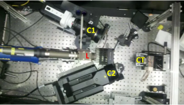
EXPERIMENTAL SETUPThe stereo rig is composed of two imaging devices (Figure 1). First, an infrared camera (x6540sc made by FLIR) with a 640 x 512 pixel definition and operating in the spectral range of wavelength λ = [3 µm-5 µm] is chosen. A 50-mm lens and a 12-mm extension ring are used. They provide a physical pixel size of 60 µm for a working distance of 18 cm. The integration time is set to 800 µs to be representative of the thermal fatigue experiments that will be monitored with such a system. In a similar spirit (Appendix A), a setup will also be tested with a high magnification lens (G1) reducing the physical pixel size to 15 µm for a working distance of 30 cm. Second, a visible light camera (MIRO M320S made by Vision Research) with a 1920 x 1080 pixel definition is also used. A Tamron SP AF180mm F/3.5 lens is chosen and leads to a physical pixel size equal to 10 µm when the working distance is set to 25 cm. The camera is sensitive to the wavelength range λ = [0.4 µm-0.8 µm]. The aperture is chosen to minimize blur effects due to the low depth of field of the lens. The exposure time is selected to be 1 ms and two 250-W Dedocool spotlights are used. The dynamic ranges of the IR and visible light cameras are 14 bits and 12 bits, respectively.
Figure 1: Top view of the hybrid stereo rig for thermal fatigue experiments: visible light (C1) and IR (C2) cameras are positioned for the calibration step. In the present case, the laser source (L) is
located between the two cameras. The calibration target (CT) is mounted on a 3-axis stage
The first configuration is using a 3-axis stage (manually) prescribing RBTs along three perpendicular directions by steps of 10µm. A second configuration is also used to apply these motions automatically (Figure 2). The latter prescribes translations with an uncertainty less than 1 µm but only along one direction (i.e., out-of-plane axis in the present case).
(a) (b)
Figure 2: Hybrid stereo configuration where RBTs are applied manually (a) or with a motorized stage in the out-of-plane direction (b)
The 3D sample is an open book target made of aluminum alloy, which was used for the calibration of an ultrahigh speed experiment [27]. Its size is 30 × 30 × 1 mm3 and the opening angle is 132°. The pattern
is made of regular white and black squares of 2.5 × 2.5 mm2 area. Only an approximate metrology of the target is available. However it will be shown that it is possible to compensate for the absence of an accurate
C2
C1
CT
(a) (b)
(c)
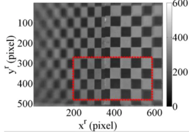
Figure 3: 3D calibration target captured by (a) the visible light and (b) the IR cameras. (c) NURBS model of the region of interest (see red boxes on both images) and the control points (red dots)
The pictures shot by the visible light (or left) camera and IR (or right) camera and the numerical model of the target are shown in Figure 3. It has to be emphasized that the IR image has undergone a change of digital levels since the white squares appear black on the row data. Further, it is worth remembering that the integration time of the IR camera is set to 800 µs, and no temperature variations are expected to occur. Therefore the full dynamic range is not exploited for this particular experiment. Because of the very long exposure to lighting, the sample temperature reaches a level of 39 °C checked to be constant during the experiment, with temperature measurements at different time intervals with the calibrated IR camera and a thermocouple measuring the temperature of the steel plate just below the open-book target.
3.
NURBS DESCRIPTION OF THE ANALYZED SURFACEEven if the cameras are operating in two different wavelength ranges, both are providing enough contrast between the “white” and “black” parts of the calibration target (see Figure 3).This is due to the fact that the emissivities of the black and white parts are different in both wavelength ranges. This property will allow for
SC calculations by resorting to a global approach. A NURBS [30] representation of the surface is defined in the parametric space (𝛼, 𝛽) ∈ [0,1]𝟐 so that any 3D point 𝐗 is described by
𝐗(𝛼, 𝛽) =∑ ∑ N𝑖,𝑝(𝛼)N𝑗,𝑞(𝛽)𝜔𝑖𝑗𝐏𝒊𝒋 𝒏 𝒋=𝟎 𝒎 𝒊=𝟎 ∑𝒎𝒊=𝟎∑𝒏𝒋=𝟎N𝑖,𝑝(𝛼)N𝑗,𝑞(𝛽)𝜔𝑖𝑗 (1) with ⩝ ∈ [0,1] ,N𝑖,0(𝛼)={ 10 otherwisewhen 𝛼𝑖≤ 𝛼 ≤ 𝛼𝑖+1 (2)
and 𝛼𝑖 are the component of the knot vector {𝛼0, … , 𝛼𝑖 , … , 𝛼𝑚}, considering 𝛼𝑖< 𝛼𝑖+1 [30] and
N𝑖,𝑝(𝛼) =
𝛼 − 𝛼𝑖
𝛼𝑖+𝑝− 𝛼𝑖N𝑖,𝑝−1(𝛼) +
𝛼𝑖+𝑝+1− 𝛼
𝛼𝑖+𝑝+1− 𝛼𝑖+1N𝑖+1,𝑝−1(𝛼) (3)
where N𝑖,𝑝 and N𝑗,𝑞 are mixing functions for each component and of the parametric space, 𝑛𝑝 = (𝑚 +
1)(𝑛 + 1) the number of control points (in the present case 𝑛𝑝= 15, see Figure 3(c)), (𝑝, 𝑞) the degrees of
the surface (here 1) and 𝐏𝐢𝐣= (XPij, YPij, ZPij) are the coordinates of the control points (or knots) of the
surface, and 𝜔𝑖𝑗 the corresponding weights (in the present case all weights are equal to 1, which reduces
the NURBS surface to a Bezier patch [30]).
4.
CALIBRATION PHASEA first calibration step of the stereo rig is performed, which consists of registering the images acquired with the IR and visible light cameras. Before performing the calibration of the stereo rig, the distortions of both imaging systems are estimated independently.
4.1 Distortions estimations
For both imaging systems the distortion corrections are performed by using integrated-DIC [39]. As numerical reference images (i.e., numerically generated for the fabrication of the calibration targets [39]) are used, gray level corrections are applied to enhance the estimation of the sought parameters [40]. The gray level correction (GLC) algorithm will also be discussed later on for the determination of projection matrices (see Section 4.2).
(a) (b)
(c)
Figure 4: Calibration target for distortion corrections. (a) Numerical reference and (b) corrected image with bilinear fields and a blurring kernel [40]. (c) Distorted image for the visible light camera
(the image definition is 1080 1920 pixels digitized with 4096 gray levels)
For the visible light camera the reference pictures before and after gray level readjustments are shown in Figure 4(a-b), which are registered with the deformed image (Figure 4(c)). The distortion estimations consist of radial, prismatic and decentering parameters [39]. The reference images are readjusted in terms of gray level by using a bilinear field (see Table 1) and one blurring kernel for both imaging systems [40].
Lens distortions induce displacement fields ux and uy shown in Figure 5. In the sequel they will be
referred to as distortion fields. To evaluate the quality of the registration DIC residuals, which are the gray level differences between the image in the reference configuration and that in the distorted configuration corrected by the distortion field, are also shown in Figure 5 for the visible light camera. As expected from the distortion model [32] the distortion fields are higher near the image borders. The levels are close to zero in the center and can reach 4 pixels (i.e., 40µm) on the edges for the displacement field along the x direction. The radial distortion parameter is equal to 16.8 pixels (when the characteristic length [39] is 1800 pixels) and the prismatic coefficients are -0.4 and 1.4 pixel along xl and yl directions. The root mean square (RMS) gray level residual is equal to 9.9% of the picture dynamic range to be compared with 35.5% when no GLCs are considered. The RMS value between the distortion fields obtained for the two calculations is 0.14 pixel for each displacement component. The remaining residuals are in large part due to local fluctuations (see Figure 4 and Figure 5(c)), which are not captured with the chosen correction fields.
(a) (b)
(c)
Figure 5: Distortion fields (a) ux and (b) uy expressed in pixels for the visible light camera. (c) Gray
level residual map at convergence. The dynamic range of the analyzed pictures is 4096 gray levels
The same method is used to estimate the distortions induced by the IR camera lens. The reference images before and after GLCs are compared with the distorted image in Figure 6. As the images are prone to blur, a Gaussian kernel is used in the gray level correction procedure [40].
(a) (b)
(c)
Figure 6: Calibration target for distortion corrections for the IR camera. (a) Numerical reference and (b) corrected image with bilinear fields and a blurring kernel [40]. (c) Distorted image (definition: 512
640 pixels digitized with 255 gray levels)
The distortion field amplitudes reach 2.4 pixels (Figure 7), which is equivalent to 144 µm in terms of physical dimensions. The dimensionless RMS gray level residual is equal to 4.6 % when GLCs are performed (to be compared with 31% when readjustments are not implemented). It is worth noting that blur is well described with the Gaussian kernel in the present case.
(a) (b)
(c)
Figure 7: Distortion fields (a) ux and (b) uy expressed in pixels for the IR camera. (c) Gray level
residual map at convergence
The acquired images, for SC purposes, are then corrected with the estimated distortion fields and are used to perform the following steps.
4.2 Projection matrices
An Integrated-SC algorithm [31] allows for the determination of the projection matrices by using a pseudo-kinematic basis. By working in the parametric space, it enables for dealing with two images of different resolutions and definitions. Consequently, the scale parameters introduced hereafter will be significantly different from each other. The pictured positions are related to the homogeneous coordinates by
{𝑠 𝑙𝑥𝑙 𝑠𝑙𝑦𝑙 𝑠𝑙 } = [𝐌𝐥]{𝐗̅} and {𝑠 𝑟𝑥𝑟 𝑠𝑟𝑦𝑟 𝑠𝑟 } = [𝐌 𝐫]{𝐗̅} (4)
target (see Figure 3(c)). An initial guess is necessary for the algorithm implemented herein. This step is performed by selecting 6 points on each image of known positions. A singular value decomposition of the system of equations (4) rewritten in terms of the unknown 3D positions is carried out and the corresponding projection matrices are determined.
In the following, it is proposed to account for the non-conservation of brightness between both imaging systems. The SC algorithm considering gray level conservation relaxation consists of minimizing the sum of squared differences over the considered region of interest (ROI) between the gray level pictures 𝑓𝑙 and 𝑓𝑟
𝛕 = ∫ [𝑓𝑟(𝐱𝐫(𝛼, 𝛽, [𝐌𝐫]) − 𝑎(𝐱𝐥(𝛼, 𝛽, [𝐌𝐥])) − (1 + 𝑏(𝐱𝐥(𝛼, 𝛽, [𝐌𝐥]))) 𝑓𝑙(𝐱𝐥(𝛼, 𝛽, [𝐌𝐥]) 𝐑𝐎𝐈 − ∑ 𝑐𝑡(𝐱𝐥(𝛼, 𝛽, [𝐌𝐥])) (𝐺𝑡∗ 𝑓𝑙) (𝐱𝐥(𝛼, 𝛽, [𝐌𝐥])) 𝑁 𝑡=1 ] 𝟐 𝑑𝛼𝑑𝛽 (5)
with respect to the components of the projection matrices and the parameterization of the brightness (𝑎) and contrast (𝑏) correction fields, as well as blurring kernels (Gaussian kernels 𝐺𝑡 in the present case) of width 𝑡
and weighting fields 𝑐𝑡 [40]. By implementing a Newton-Raphson scheme it is then possible to update the
corrected image 𝑔𝑛+1(𝐱𝐥) = 𝑎𝑛(𝐱𝐥) + 𝑑𝑎(𝐱𝐥) + (1 + 𝑏𝑛(𝐱𝐥) + 𝑑𝑏(𝐱𝐥)) ∙ 𝑓𝑙(𝐱𝐥) + ∑(𝑐 𝑡𝑛(𝐱𝐥) + 𝑑𝑐𝑡(𝐱𝐥))(𝐺𝑡∗ 𝑓𝑙)(𝐱𝐥) 𝑁 𝑡=1 (6)
after each iteration n as the result of the solution to a linear system
[𝐊𝐧]{𝐝𝐦} = {𝐫𝐧} (7)
where the corrections to the unknown amplitudes are gathered in the column vector {𝐝𝐦}
{𝐝𝐦}𝒕= {{𝐝𝐌}t, {𝐝𝐚}t, {𝐝𝐛}t, {𝐝𝐜}t} (8)
in which the column vector {𝐝𝐌} gathers all components of the corrections to the projection matrices but 𝑀34𝑙,𝑟, which are set to the value determined from the singular value decomposition. Its size is 22 × 1. The
column vector {𝐝𝐚} contains na amplitude corrections associated with the chosen brightness correction fields,
corrections associated with the parameterization of all the weighting fields of the Gaussian kernels. The (22+na+nb+Nnc) × (22+na+nb+Nnc) SC matrix reads
[𝐊𝐧] = ∫{𝐤𝐧}{𝐤𝐧}𝑡𝑑𝛼𝑑𝛽 𝑅𝑂𝐼
(9)
and the corresponding (22+na+nb+Nnc) × 1 residual vector
{𝐫𝐧} = ∫{𝐤𝐧}( 𝑓𝑟 − 𝑔𝑛)𝑑𝛼𝑑𝛽 𝑅𝑂𝐼
(10)
for which {𝐤𝐧} is defined for each evaluation point x of the parametric space as
{𝐤𝐧}𝒕= {{𝚿𝒍}𝑡, {𝚿𝒓}𝑡, {𝛗}𝑡, {𝛟}𝑡, {𝚽}𝑡} (11)
where {𝚿𝒍} is the column vector that gathers all 11 scalar products (𝝍𝑖𝑗𝑙 ∙ 𝛁𝑓)(𝐱), {𝚿𝒓} the corresponding column vector of the 11 scalar products (𝝍𝑖𝑗𝑟 ∙ 𝛁𝑔𝒏)(𝐱), {𝛗} the column vector containing na values of
interpolation fields 𝜑𝑘(𝐱) for GLCs [40], {𝛟} the column vector gathering nb products 𝜑𝑘(𝐱)𝑔(𝐱), and {𝚽} the
column vector containing Nnc products 𝜑𝑘(𝐱)(𝐺𝑡∗ 𝑔)(𝐱). The sensitivities 𝝍𝑖𝑗𝑙,𝑟 of 𝐱𝐥,𝐫 to the sought
components 𝑀𝑖𝑗𝑙,𝑟 of the projection matrices [31] are expressed as
𝝍𝑖𝑗𝑙,𝑟= ∂𝐱𝐥,𝐫 ∂𝑀𝑖𝑗𝑙,𝑟 𝑑𝑀𝑖𝑗𝑙,𝑟 (12) with {𝐱l,r }= { 𝑥𝑙,𝑟 =𝑀1𝑖𝑙,𝑟𝐗𝒊(𝛼,𝛽) 𝑀3𝑖𝑙,𝑟𝐗𝒊(𝛼,𝛽) 𝑦𝑙,𝑟 =𝑀2𝑖𝑙,𝑟𝐗𝒊(𝛼,𝛽) 𝑀3𝑖𝑙,𝑟𝐗𝒊(𝛼,𝛽)} (13)
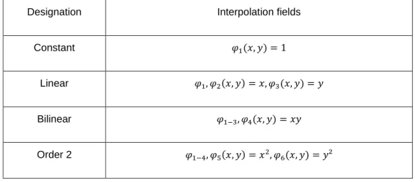
In the present case, low order polynomials are selected for the 𝜑𝑘 interpolation fields (Table 1). Last, all
Table 1: Interpolation fields used for gray level corrections and blur effects
Designation Interpolation fields
Constant 𝜑1(𝑥, 𝑦) = 1
Linear 𝜑1, 𝜑2(𝑥, 𝑦) = 𝑥, 𝜑3(𝑥, 𝑦) = 𝑦
Bilinear 𝜑1−3, 𝜑4(𝑥, 𝑦) = 𝑥𝑦
Order 2 𝜑1−4, 𝜑5(𝑥, 𝑦) = 𝑥2, 𝜑6(𝑥, 𝑦) = 𝑦²
It is now possible to perform an SC analysis to evaluate the projection matrices of both cameras.
4.3 Influence of gray level correction and distortion effects
The gray level conservation assumption between both images is investigated in terms of errors induced on the projection matrices. When the gray levels are assumed to be conserved, the RMS gray level residual is as high as 28.6 % of the dynamic range. When second order fields are considered and one blurring kernel it reduces to 0.9% (Figure 8).
(a) (b)
Figure 8: Gray level residual for the determination of the projection matrices (a) without and (b) with gray level corrections and blur (see main text)
In order to assess the influence of GLCs (without lens distortion corrections), the two left matrices corresponding to the visible light camera are shown without GLC
[𝐌𝐥] = [−0.360.4 0.0 −40.2 −0.8 0.0 −0.2 −71.5 0.0 687.8 718.8 0.7 ] ∙ 10 −3 and with GLC
[𝐌𝐆𝐋𝐂𝐥 ] = [ 59.7 −0.6 0.0 −41.7 −1.2 0.0 −0.1 −71.4 0.0 687.9 718.8 0.7 ] ∙ 10 −3
so that their absolute difference reads
[𝐚𝐛𝐬(∆𝐌𝐥)] = [0.70.2 0.0 1.5 0.5 0.0 0.1 0.1 0.0 0.0 0.0 0.0 ] ∙ 10 −3
Except for one component, the differences do not exceed 10-3. Therefore, the results are not very sensitive to the fact that the gray levels have been readjusted.
For the right matrix corresponding to the IR camera the projection matrices before corrections
[𝐌𝐫] = [−2.540.6 0.1 −90.1 −89.7 −0.2 −4.8 −3.3 0.0 511.8 879.0 −1.7 ] ∙ 10−3 and after GLCs [𝐌𝐆𝐋𝐂𝐫 ] = [ −28.6 1.2 0.0 −18.3 −1.1 0.0 −1.1 −33.3 0.0 534.0 845.4 −1.7 ] ∙ 10 −3
are significantly different
[𝐚𝐛𝐬(∆𝐌𝐫)] = [26.139.4 0.1 71.7 90.7 0.2 3.7 0.1 0.0 22.2 33.6 0.0] ∙ 10 −3
It is worth noting that the initial guess was closer to the matrices determined with GLC. It is concluded that GLCs should be accounted for.
The distortion effects are also investigated. The gray level difference between distorted and corrected images is calculated (Figure 9). The RMS residuals are respectively equal to 1.3% and 2.7% of the dynamic range for the visible light and IR cameras, which remain very low on average. The corresponding maps are more biased when reaching the edges and corners of the pictures.
The new projection matrix considering distortion corrections (DC) for the visible light (i.e., left) camera is [𝐌𝐃𝐂_𝐆𝐋𝐂𝐥 ] = [ 60.2 −0.2 0.0 −41.0 −1.3 0.0 −0.1 −71.4 0.0 687.7 719.0 0.7 ] ∙ 10 −3
and that for the IR (i.e., right) camera reads
[𝐌𝐃𝐂_𝐆𝐋𝐂𝐫 ] = [ −28.3 1.3 0.0 −17.6 −1.7 0.0 −0.9 −33.7 0.0 533.2 844.8 −1.7 ] ∙ 10 −3
When compared to the previously determined values while only assessing the effects of GLCs, their absolute differences are for the left camera
[𝐚𝐛𝐬(∆𝐌𝐃𝐂_𝐆𝐋𝐂𝐥 )] = [ 0.5 0.4 0.0 0.7 0.1 0.0 0.0 0.0 0.0 0.2 0.2 0.0 ] ∙ 10 −3
and for the right camera
[𝐚𝐛𝐬(∆𝐌𝐃𝐂_𝐆𝐋𝐂𝐫 )] = [ 0.3 0.1 0.0 0.70.6 0.0 0.2 0.4 0.0 0.80.8 0.0 ] ∙ 10−3
In comparison with the previous analysis, the differences are about one order of magnitude lower.
The GLCs and the distortion effects have been investigated for the projection matrices during the calibration step. It is shown that there is an effect on the sought parameters when GLCs are accounted for. In the present case the correction of distortions does not show significant differences in terms of projection matrix estimations. Let us also stress that in both of these projection matrices, there is a scale factor that is not determined by image registration, but rather by setting an absolute dimension of the target. At the present stage, only an approximate value has been used because a precise target metrology is not available. However, as shown below, the measurement of RBTs may compensate for such difficulty.
5.
RIGID BODY TRANSLATION MEASUREMENTThe calibration procedure allowed the projection matrices to be determined. The images shot by the IR and visible light cameras can be interpolated in the parametric space of the NURBS model. To measure displacement fields, the algorithm consists of simultaneously minimizing two global residuals, namely, those of the left pair of images and right pair of images with respect to the kinematic unknowns, which are the pole motions of the surface model. It is also proposed to reduce the number of degrees of freedom by assuming that the motion reduces to a rigid body translation via integrated SC.
5.1 3D displacement measurement
𝛕 = ∫[𝑓𝑙(𝐱𝐥(𝛼, 𝛽, 𝐏 𝐢𝐣) − 𝑔𝑙(𝐱𝐥(𝛼, 𝛽, 𝐏𝐢𝐣+ 𝐝𝐏𝐢𝐣)] 𝟐 𝑑𝑢𝑑𝑣 𝑹𝑶𝑰 + ∫[𝑓𝑟(𝐱𝐫(𝛼, 𝛽, 𝐏 𝐢𝐣) − 𝑔𝑟(𝐱𝐫(𝛼, 𝛽, 𝐏𝐢𝐣+ 𝐝𝐏𝐢𝐣)] 𝟐 𝑑𝛼𝑑𝛽 𝑹𝑶𝑰 (14)
where 𝐏𝐢𝐣 are the initial position of the control points of the NURBS surface (i.e., 3n𝑝 coordinates). The
displacement fields are then obtained by estimating the motions 𝐝𝐏𝐢𝐣 of the control points in the “deformed” images gl,r with respect to the reference images fl,r. Since the measurements are performed at room temperature, the gray and digital level conservation is assumed to remain satisfied up to acquisition noise and small illumination variations. A Newton-Raphson algorithm is implemented to minimize the previous functional. For a given iteration, the linear equations to solve read
[𝐂]{𝐝𝐩} = {𝛒} (15)
where the 3n𝑝× 3n𝑝 SC matrix is expressed as
[𝐂] = ∫ ({𝐬𝐥}{𝐬𝐥}𝑡+ {𝐬𝐫}{𝐬𝐫}𝑡) 𝑹𝑶𝑰
𝑑𝛼𝑑𝛽 (16)
with {𝐬𝒍,𝒓} the column vectors that gather all 3n𝑝 scalar products of the sensitivity fields 𝛛𝐱
𝐥,𝐫
𝛛𝐏𝐢𝐣 with the
corresponding picture contrast 𝛁𝑓𝑟,𝑙 for each evaluation point 𝐱𝐥,𝐫(𝛼, 𝛽) in the parametric space, {𝐝𝐩} the column vector containing all 3n𝑝 incremental motions of the considered control points, and the 3n𝑝 × 1 SC
column vector
{𝛒} = ∫({𝐬𝐥}(𝑓𝑙− 𝑔̃𝑙) + {𝐬𝐫}(𝑓𝑟− 𝑔̃𝑟)) 𝑹𝑶𝑰
𝑑𝛼𝑑𝛽 (17)
for the current iteration, namely, for the pictures 𝑔̃𝑙,𝑟 in the deformed configuration corrected by the current estimate of pole motions. In the present case, the algorithm is initialized by assuming that no motions have occurred.
5.2 Integrated approach
[𝐂𝑹𝑩𝑻] = [𝚪]𝒕[𝐂][𝚪] (18) where [𝚪] is a 3n𝑝 × 3 matrix [𝚪] = [ {𝟏} {𝟎} {𝟎} {𝟎} {𝟏} {𝟎} {𝟎} {𝟎} {𝟏}] (19)
with {𝟎} a column vector containing n𝑝 zeros, and {𝟏} a column vector containing n𝑝 ones. The reduced 3 × 1
SC residual vector then reads
{𝛒𝑹𝑩𝑻} = [𝚪]𝒕{𝛒} (20)
This new setting reduces the number of kinematic unknowns from 3n𝑝 to three translations to be determined
directly with no additional reprojection.
5.3 Measurement results
First, it is necessary to assess the resolution of the SC code. The displacement fields between two sets of images where no experimental RBT is applied are measured. The standard resolution is estimated via the standard deviation of the measured displacement fields, which is equal to 0.4 µm along the three perpendicular directions.
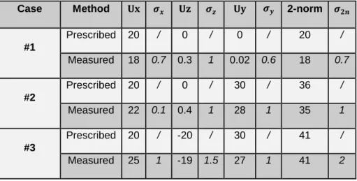
The target is first moved by using a manual 3-axis stage. The prescribed and measured RBTs are listed in Table 2. As the measurement results are displacement fields, the averages (Ux, Uy, Uz) are listed and the corresponding standard deviations (𝜎𝑥, 𝜎𝑦, 𝜎𝑧). Three different cases are analyzed, which consist of
translations along one, two and three directions. The maximum amplitude is equal to 41 µm. Let us mention that the translation stage has been only grossly aligned with the 3D frame used for the target representation. All results will be expressed in the stage frame for the prescribed displacements, and in the target frame for the measured displacements. For comparison purposes, the L2-norm of the displacements, which is independent of the considered frame, is also reported.
Table 2: Prescribed and measured rigid body motions expressed in µm Case Method 𝐔𝐱 𝝈𝒙 𝐔𝐳 𝝈𝒛 𝐔𝐲 𝝈𝒚 2-norm 𝝈𝟐𝒏
#1 Prescribed 20 / 0 / 0 / 20 / Measured 18 0.7 0.3 1 0.02 0.6 18 0.7 #2 Prescribed 20 / 0 / 30 / 36 / Measured 22 0.1 0.4 1 28 1 35 1 #3 Prescribed 20 / -20 / 30 / 41 / Measured 25 1 -19 1.5 27 1 41 2
According to the average values reported in Table 2, the displacement fields are well captured and the standard displacement uncertainties are very low, namely, in the micrometer range. The difference in terms of mean displacement component is mostly due to misalignments between the target frame and that of the 3-axis stage. However, when expressed in terms of the L2-norm, which is immune from such misalignments, the mean errors are lowered.
The remaining gaps may result from different sources. The displacement fields show a gradient near the borders that should not appear as only RBTs are applied. Different reasons can explain such effects. The first one is the presence of distortion on the images used for these first results, which are not corrected. These fluctuations can also be related to blur, which are more important near the image edges as the depth of field is low for both cameras (Figures 4 and 6). Finally the knot motions can be due to the fine discretization used, namely 1,000 by 1,000 evaluation points compared to the pattern of the calibration target (large squares covering large number of pixels).
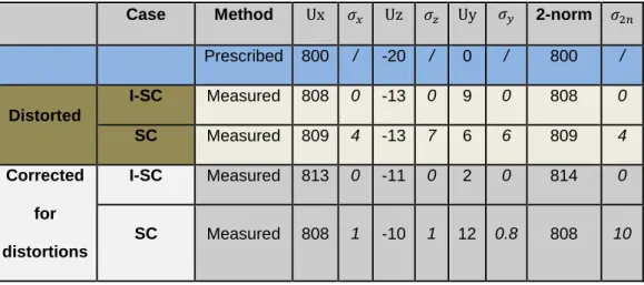
The comparison between SC and I-SC approaches is now studied. In addition the distortion effects are also investigated and the results are summarized in Table 3. Both approaches provide close results, namely, the RMS difference of the amplitudes is equal to 2 µm. The results are also very close to the prescribed RBTs. Similarly, the distortion corrections do not seem to significantly improve the final results for both methods. The effect of blur is not investigated herein, in order to minimize such effects the I-SC calculations will be used in the following discussions.
Table 3: Prescribed and measured rigid body motions expressed in µm Case Method Ux 𝜎𝑥 Uz 𝜎𝑧 Uy 𝜎𝑦 2-norm 𝜎2𝑛
Prescribed 800 / -20 / 0 / 800 / Distorted I-SC Measured 808 0 -13 0 9 0 808 0 SC Measured 809 4 -13 7 6 6 809 4 Corrected for distortions I-SC Measured 813 0 -11 0 2 0 814 0 SC Measured 808 1 -10 1 12 0.8 808 10
The L2-norm results with I-SC corrected for distortions overestimate the prescribed displacement by about 1.8 %. This small difference is due to the scale factor that was set with an approximate estimate of the absolute size of the calibration target. With the present procedure, more faithful estimates of the scale factors are obtained. The scale factor is readjusted by enforcing the L2-norm of the measured translation to be equal to the prescribed value (here 800 µm). As a way of validating the results, a second test case (i.e., smaller displacement) is also reported in Table 4. The resulting L2-norm is closer to the prescribed value (the relative error decreases from about 5 % to 1.5 %). Yet, the gap in terms of displacement components is high compared to their respective L2-norms. This is clearly the effect of the misalignment of the coordinate system.
Table 4: Prescribed and measured RBTs expressed in µm before and after correcting the scale factor by resorting to I-SC with distortion corrections
Scale factor Method Ux Uz Uy 2-norm Prescribed 800 -20 0 800 as calibrated Measured 813 -11 2 814 Readjusted Measured 800 -12 6 800 Prescribed 200 -20 0 201 as calibrated Measured 210 -16 2 211 Readjusted Measured 203 -23 2 204
RBTs are now prescribed with an automated stage in only one direction. Successive amplitudes have been applied along an out-of-plane direction. I-SC is selected for the sake of simplicity. As long as the prescribed motions are lower than 5 µm no displacement is detected. When a 5-µm amplitude is applied, the L2-norm of the measured translation is equal to 6.1 µm. This means that for this camera configuration and the observed object the absolute difference is about 1 µm, which is considered to be very low given the quality of the pattern [41] (i.e., the size of the elementary squares are much bigger than that of the pixels) and the physical pixel sizes (i.e., 60 µm and 10 µm for the IR and visible light cameras, respectively). When an amplitude of 81.0 µm is prescribed, the L2-norm of the measured translation is 81.1 µm, which remains very close. When higher levels are applied the discrepancy between measured and prescribed displacement increases.
This effect can be explained by the imperfect alignment between the model and the stage coordinates, as well as the above discussed scale factor that is not set from the calibration. Both artifacts can be corrected from the measured data. If each measured displacement component 𝑈𝑖𝑚𝑒𝑎𝑠 is adjusted as an affine
form of the prescribed displacement 𝑈𝑗𝑝𝑟𝑒𝑠 performed along an orthogonal direction
𝑈𝑖𝑚𝑒𝑎𝑠= 𝑎𝑖𝑈𝑗𝑝𝑟𝑒𝑠+ 𝑏𝑖 (21)
then a corrected displacement 𝑈𝑖𝑐𝑜𝑟𝑟 is estimated as the residual
𝑈𝑖𝑐𝑜𝑟𝑟= 𝑈𝑖𝑚𝑒𝑎𝑠− 𝑎𝑖𝑈𝑗𝑝𝑟𝑒𝑠− 𝑏𝑖 (22)
for i = x, y or z and i ≠ j (where the assumption of a misalignment angle has been used). In the present cases
i = x or y and j= z. For a scale factor readjustment the corrected displacement reads
𝑈𝑧𝑐𝑜𝑟𝑟 =
𝑈𝑧𝑚𝑒𝑎𝑠− 𝑏𝑧
𝑎𝑧
(23)
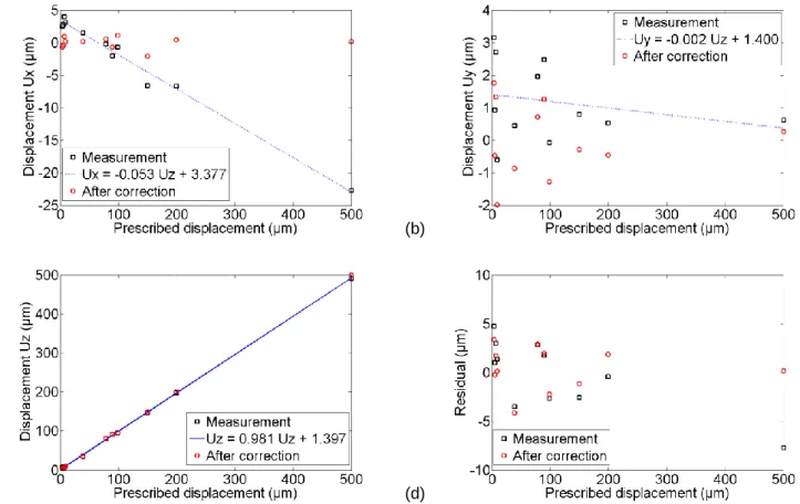
Figure 10 shows the original (i.e., raw) measured data, the linear regression, and the corrected displacement data. Figure 10(c) shows the measurement, the linear regression through the data, and the corrected displacement along the z axis, whereas the L2-norm residuals are shown in Figure 10(d). It can be seen that 𝑈𝑥𝑚𝑒𝑎𝑠 levels are impacted by the misalignment (Figure 10(a)) with an angle of 3.1° while 𝑈𝑦𝑚𝑒𝑎𝑠 components
5 µm for the different components. Last, the RMS error associated with L2-norm of the displacement decreases from 3.5 µm to 2.1 µm. The automated translation stage is accurate down to the micrometer level, which thus is not limiting here. Let us note that a mere correction for scale and alignment based on the two extreme measurements would provide a comparable result, and is much less demanding in terms of data processing. All the intermediate measurements then become validation points for the calibration procedure. Further, this procedure is an easy way to circumvent the difficulty of not having a micrometer metrology of the calibration target. It is worth noting that it was used to prove the feasibility of the proposed hybrid framework. The fact that the target is moving is, in a sense, a self-calibration procedure, which is very advantageous for, say, large structures but also in the present case. The uncertainties are assessed for the object of interest (i.e., here the calibration target). They have to be re-evaluated for the true experiment since a different (random) pattern would be used instead.
(a) (b)
(c) (d)
Figure 10: Measured translations along the X (a) and Y (b) directions versus the prescribed out-of-plane motions before and after corrections. The estimated RBTs along the Z axis and the residuals of
the L2-norm of the measured displacements against the prescribed motions are respectively plotted in subfigures (c) and (d)
The gray level residuals obtained for the two image pairs are shown in Figure 11 for the largest displacement (i.e., 500 µm); similar maps are observed for the other cases. The RMS gray level residuals normalized by the dynamic range of the reference picture are smaller for the visible light camera (0.3 to 1.5 %) when compared with the IR camera (0.8 to 8.31 %) when 3D displacements are measured. These small levels and the corresponding maps (Figure 11) indicate that the registration was successful. For the 3D displacement measurements, the GLCs are less crucial than in the calibration step since the registration is performed on pictures shot by the same imaging system (registration of image pairs acquired by the same imaging device, IR/IR and visible light/visible light, see Equation (14)). Conversely, when the temperature (that of the observed sample as well as that of the surrounding) varies, the reference and deformed IR images will experience digital level variations, which can be interpreted in terms of temperature fields by adding new variation fields, whose spatial fluctuations may, for example, be described by finite element discretization of the temperature field [25].
(a) (b)
Figure 11: Residual errors for the visible light camera (𝑓𝑙− 𝑔̃𝑙) expressed in gray levels (a) and IR
camera (𝑓𝑟− 𝑔̃𝑟) expressed in digital levels (b) when a 500-µm displacement was applied
6.
CONCLUSIONS AND PERSPECTIVESIsogeometric SC is developed on a hybrid stereo rig made of two different imaging systems, namely, one IR camera and one visible light camera. The calibration step is performed by using the NURBS model of the calibration target. Working in the parametric space of the 3D surface allows for easily handling two images of different definition and resolution. In the present case, the typical pixel size is about six times smaller for the visible light camera in comparison with the IR camera. SC analyses could be performed
precisely, its exact metrology to estimate the scale factors. The gray level readjustment, which accounts for brightness/contrast variations and blur, provides very low residual errors, namely, 1 % of the dynamic range (against 29 %). Its impact on the projection matrices is not negligible. At this stage the projection matrices are better estimated with such corrections. The distortion corrections have also been applied to both imaging systems. In the present case, no significant improvement is observed.
The displacement fields are measured with a micrometer standard uncertainty for a range of 40 µm and when the amplitude increases to 800 µm. The amplitudes of the translation vector are well captured even when the 3D model axes are not aligned with those of the translation stages, while the displacement components are altered by rotations. Both global SC and I-SC approaches provided similar results. No sensitivity to distortion corrections have been observed for this configuration. Using I-SC allowed for accelerating the computation time and avoiding spurious pole motions on the ROI edges (resulting either from the presence of blur, which induces a loss of information, or from too fine a discretization of the parametric space). By using I-SC, the initial calibration of the scale factors could be corrected by prescribing displacement with micrometric uncertainty.
I-SC was then used to measure out-of-plane motions using an automated stage prescribing micrometric displacements. For motion amplitudes below 5 µm the measurements are mostly corrupted by noise. Misalignment and absolute scale adjustments can be corrected for based on this displacement measurement for larger amplitudes. Final values of standard discrepancies between prescribed and measured displacements are in the range 2-3 µm for displacements amplitudes up to 800 µm.
All these results prove the feasibility of SC analyses with a hybrid system made of one IR camera and one visible light camera. The next step will be to account for digital level variations of the IR camera when temperature variations occur. This would allow for combined and totally synchronized measurements of 2D temperature fields and 3D displacement fields with only two cameras.
Blur due to defocusing, which was not addressed at this stage, should also be added in the analysis. Second, refined gray and digital level corrections should be implemented, in particular to account for local temperature variations induced by laser shocks. Further, samples on which laser shocks are applied are stainless steel plates with a pattern provided by natural pre-oxidation. The next challenges will then be to calibrate with 2D surfaces in order to be able to measure 3D displacement fields that occur very locally with amplitudes of a few micrometers. In order to have a better spatial resolution a G1-lens will be used for the IR camera (see Appendix A). All these new challenges will have to be met if the system is to be used to monitor such types of experiments [6].
7.
REFERENCES[1] A. Amiable, S. Chapuliot, S. Contentinescu, and A. Fissolo, “A computational lifetime prediction for a thermal shock experiment, Part I: Thermomechanical modeling and lifetime prediction,” Fatigue Fract.
Eng. Mater. Struct., vol. 29, pp. 209–217, 2006.
[2] A. Fissolo, S. Amiable, O. Ancelet, F. Mermaz, J. M. Stelmaszyk, A. Constantinescu, C. Robertson, L. Vincent, V. Maillot, and F. Bouchet, “Crack initiation under thermal fatigue: An overview of CEA experience. Part I: Thermal fatigue appears to be more damaging than uniaxial isothermal fatigue,” Int.
J. Fatigue, vol. 31, no. 3, pp. 587–600, Mar. 2009.
[3] A. Fissolo, C. Gourdin, O. Ancelet, S. Amiable, A. Demassieux, S. Chapuliot, N. Haddar, F. Mermaz, J. M. Stelmaszyk, A. Constantinescu, L. Vincent, and V. Maillot, “Crack initiation under thermal fatigue: An overview of CEA experience: Part II (of II): Application of various criteria to biaxial thermal fatigue tests and a first proposal to improve the estimation of the thermal fatigue damage,” Int. J. Fatigue, vol. 31, no. 7, pp. 1196–1210, Jul. 2009.
[4] L. Vincent, M. Poncelet, S. Roux, F. Hild, and D. Farcage, “Experimental Facility for High Cycle Thermal Fatigue Tests Using Laser Shocks,” Fatigue Des. 2013 Int. Conf. Proc., vol. 66, no. 0, pp. 669–675, 2013.
[5] C. Esnoul, L. Vincent, M. Poncelet, F. Hild, and S. Roux, “On the use of thermal and kinematic fields to identify strain amplitudes in cyclic laser pulses on AISI 304L strainless steel,” presented at the Photomechanics, Montpellier (France), 2013.
[6] A. Charbal, L. Vincent, F. Hild, M. Poncelet, J.-E. Dufour, S. Roux, and D. Farcage, “Characterization of temperature and strain fields during cyclic laser shocks,” Quant. InfraRed Thermogr. J.. DOI: 10.1080/17686733.2015.1077544, 2015.
[7] M. A. Sutton, J.-J. Orteu, and H. W. Schreier, Image Correlation for Shape,Motion and Deformation
Measurements. Springer, 2009.
[8] J.-J. Orteu, “3-D computer vision in experimental mechanics,” Opt. Meas., vol. 47, no. 3–4, pp. 282–291, Mar. 2009.
[9] F. Hild and S. Roux, “Digital Image Correlation,” in Optical Methods for Solid Mechanics : A Full-Field
Approach, Wiley-VCH, Berlin (Germany). P. Rastogi and Editor E. Hack (Edts.), 2012.
[10] S. Prakash, P. Y. Lee, and A. Robles-Kelly, “Stereo techniques for 3D mapping of object surface temperatures,” Quant. InfraRed Thermogr. J., vol. 4, no. 1, pp. 63–84, Jun. 2007.
[11] J. Rangel, S. Soldan, and A. Kroll, “3D Thermal Imaging: Fusion of Thermography and Depth Cameras,” presented at the 12th International Conference on Quantitative Infrared Thermography, Bordeaux, 2014. [12] G. Gaussorgues, La thermographie infrarouge, 4th ed. TEC&DOC, 1999.
[13] J.-J. Orteu, Y. Rotrou, T. Sentenac, and L. Robert, “An Innovative Method for 3-D Shape, Strain and Temperature Full-Field Measurement Using a Single Type of Camera: Principle and Preliminary Results,” Exp. Mech., vol. 48, no. 2, pp. 163–179, Apr. 2008.
[14] A. Chrysochoos and G. Martin, “Tensile test microcalorimetry for thermomechanical behaviour law analysis,” Mater. Sci. Eng. A, vol. 108, no. 0, pp. 25–32, Feb. 1989.
[15] D. Favier, H. Louche, P. Schlosser, L. Orgéas, P. Vacher, and L. Debove, “Homogeneous and heterogeneous deformation mechanisms in an austenitic polycrystalline Ti–50.8 at.% Ni thin tube under tension. Investigation via temperature and strain fields measurements,” Acta Mater., vol. 55, no. 16, pp. 5310–5322, Sep. 2007.
[16] P. Schlosser, H. Louche, D. Favier, and L. Orgéas, “Image Processing to Estimate the Heat Sources Related to Phase Transformations during Tensile Tests of NiTi Tubes,” Strain, vol. 43, no. 3, pp. 260– 271, Aug. 2007.
[17] A. Chrysochoos, B. Berthel, F. Latourte, A. Galtier, S. Pagano, and B. Wattrisse, “Local energy analysis of high-cycle fatigue using digital image correlation and infrared thermography,” J. Strain Anal. Eng.
Des., vol. 43, no. 6, pp. 411–422, Jun. 2008.
[18] A. Chrysochoos, “Thermomechanical Analysis of the Cyclic Behavior of Materials,” IUTAM Symp.
Full-Field Meas. Identif. Solid Mech., vol. 4, no. 0, pp. 15–26, 2012.
[19] L. Bodelot, L. Sabatier, E. Charkaluk, and P. Dufrénoy, “Experimental setup for fully coupled kinematic and thermal measurements at the microstructure scale of an AISI 316L steel,” Mater. Sci. Eng. A, vol. 501, no. 1–2, pp. 52–60, Feb. 2009.
[22] R. Seghir, L. Bodelot, E. Charkaluk, and P. Dufrénoy, “Numerical and experimental estimation of thermomechanical fields heterogeneity at the grain scale of 316L stainless steel,” Comput. Mater. Sci., vol. 53, no. 1, pp. 464–473, Feb. 2012.
[23] S. Utz, E. Soppa, K. Christopher, X. Schuler, and H. Silcher, “Thermal and mechanical fatigue loading - Mechanisms of crack initiation and crack growth,” presented at the Proceedings of the ASME 2014 Pressure Vessels & Piping Conference, PVP2014, Anaheim, California, USA, 2014, p. 10.
[24] T. Pottier, M.-P. Moutrille, J.-B. Le Cam, X. Balandraud, and M. Grédiac, “Study on the Use of Motion Compensation Techniques to Determine Heat Sources. Application to Large Deformations on Cracked Rubber Specimens,” Exp. Mech., vol. 49, no. 4, pp. 561–574, Aug. 2009.
[25] A. Maynadier, M. Poncelet, K. Lavernhe-Taillard, and S. Roux, “One-shot Measurement of Thermal and Kinematic Fields: InfraRed Image Correlation (IRIC),” Exp. Mech., vol. 52, no. 3, pp. 241–255, Mar. 2012.
[26] A. Maynadier, M. Poncelet, K. Lavernhe-Taillard, and S. Roux, “One-shot thermal and kinematic field measurements: Infra-Red Image Correlation,” in Application of Imaging Techniques to Mechanics of
Materials and Structures, Volume 4, T. Proulx, Ed. Springer New York, 2013, pp. 243–250.
[27] G. Besnard, J.-M. Lagrange, F. Hild, S. Roux, and C. Voltz, “Characterization of Necking Phenomena in High-Speed Experiments by Using a Single Camera,” EURASIP J. Image Video Process., vol. 2010, no. 1, 215956, 2010.
[28] R. Szeliski, Computer Vision: Algorithms and Applications. Springer, 2010.
[29] J.-E. Dufour, B. Beaubier, F. Hild, and S. Roux, “CAD-based Displacement Measurements with Stereo-DIC : Principle and First Validations,” Exp. Mech., vol. 55, no. 9, pp. 1657–1668, Nov. 2015.
[30] L. Piegl and W. Tiller, The NURBS Book, 2nd ed. Springer, 1997.
[31] B. Beaubier, J.-E. Dufour, F. Hild, S. Roux, S. Lavernhe, and K. Lavernhe-Taillard, “CAD-based calibration and shape measurement with stereoDIC,” Exp. Mech., vol. 54, no. 3, pp. 329–341, Mar. 2014.
[32] D. C. Brown, “Decentering distortion of lenses,” Photogrammetric Engineering, pp. 444–462, 1966. [33] D. C. Brown, “Close-range camera calibration,” Photogrammetric Engineering, pp. 855–866, 1971. [34] O. D. Faugueras and G. Toscani, “The Calibration Problem for Stereoscopic Vision,” in Sensor Devices
and Systems for Robotics, vol. 52, A. Casals, Ed. Springer Berlin Heidelberg, 1989, pp. 195–213.
[35] R. Y. Tsai, “Versatile camera calibration technique for high-accuracy 3D machine vision metrology using off-the shelf TV cameras and lenses,” pp. 323–344, 1987.
[36] C. S. Fraser, “Digital camera self-calibration,” ISPRS J. Photogramm. Remote Sens., vol. 52, no. 4, pp. 149–159, Aug. 1997.
[37] C. S. Fraser, “Automated Processes in Digital Photogrammetric Calibration, Orientation, and Triangulation,” Digit. Signal Process., vol. 8, no. 4, pp. 277–283, Oct. 1998.
[38] J. Salvi, X. Armangué, and J. Batlle, “A comparative review of camera calibrating methods with accuracy evaluation,” Pattern Recognit., vol. 35, no. 7, pp. 1617–1635, Jul. 2002.
[39] J.-E. Dufour, F. Hild, and S. Roux, “Integrated digital image correlation for the evaluation and correction of optical distortions,” Opt. Lasers Eng., vol. 56, pp. 121–133, 2014.
[40] A. Charbal, J.-E. Dufour, A. Guery, F. Hild, S. Roux, L. Vincent, and M. Poncelet, “Integrated Digital Image Correlation considering gray level and blur variations: Application to distortion measurements of IR camera,” Opt. Lasers Eng., vol. 78, pp. 75–85, Mar. 2016.
[41] G. Crammond, S. W. Boyd, and J. M. Dulieu-Barton, “Speckle pattern quality assessment for digital image correlation,” Opt. Lasers Eng., vol. 51, no. 12, pp. 1368 – 1378, 2013.
APPENDIX A: HYBRID STEREORIG AT HIGHER MAGNIFICATION
In order to have a better spatial resolution, a G1 lens may also be used for the IR camera (FLIR x6540sc, 640x512 pixels, pitch = 15µm). The observed sample imposes the latter to be positioned normal to its surface (see Figure A1) due to the low depth of field.
Figure A1: Hybrid stereo rig with the IR (with G1 lens) and visible light cameras where the motions are manually applied along 3 axes
The IR camera with a G1-lens is calibrated by following the same procedure as above. Since the previous 2D target does not provide sufficient contrast at room temperature, another one is used for the distortion corrections. A grid made of copper is deposited onto a black painted surface. The difference of emissivities (i.e., low for copper and high for the black paint) provides the required contrast. According to the manufacturer the pitch is 480 µm so that a simple grid is generated. The latter is used as a reference in the boxed region of interest (ROI) of Figure A2.
The measured distortion fields are illustrated in Figure A3. As observed with the visible light camera, they are vanishing in the image center and reach 1.5 pixel (or 22.5 µm) near the image borders. Even when expressed in pixels, these orders of magnitude are lower than those observed with the 50-mm lens, thereby proving that the quality of the G1-lens is higher than the 50-mm lens with the 12mm extension ring.
(a) (b)
Figure A3: Distortion fields (a) ux and (b) uy (expressed in pixel) for the IR camera with G1 lens
Once the pictures are corrected from the estimated lens distortions, it is possible to perform the next step, which consists of determining the projection matrices. When the gray levels are assumed to be conserved, the RMS gray level residual is as high as 25.1 % of the dynamic range. When a second order field (polynomial function of order 2) is considered and one blurring kernel it is reduced to 1.2%. The quality of the residual after GLC corrections (see Figure A4) is an additional proof of the quality of the estimates.
(a) (b)
Figure A4: Gray level residual for the determination of the projection matrices (a) without and (b) with gray level and blur corrections (see main text)
Similar remarks and conclusions can be drawn from the present study, namely, the initial guess is closer to the matrices determined with GLC and that such corrections should be considered for a better
The translational motions are performed by using a manual 3-axis stage. The prescribed and measured rigid body motions are listed in Table A1. In the present case, the integrated version (I-SC) is considered. According to the values reported in Table A1, the displacements are well captured. The difference in terms of displacement component is mostly due to misalignments between the target frame and that of the 3-axis stage.
Table A1: Prescribed and measured rigid body motions expressed in µm
Case Ux Uy Uz 2-Norm #1 Prescribed 30 0 0 30 Measured 26 -1 -8 27 #2 Prescribed 30 0 -30 42 Measured 31 -2 -28 42 #3 Prescribed 30 0 -50 58 Measured 34 -1 -47 58
Globally, the I-SC residuals normalized by the dynamic range of the reference pictures are smaller for the visible light camera (ranging from 0.6 to 1.2 %) when compared with the IR camera (0.6 to 2.1 %) when 3D displacements are measured. These low levels and the fact that the residual map is rather uniform (Figure A5(b)) when compared to the case with no GLCs (Figure A5(a)) show that the registration was successful.
(a) (b)
Figure A5: Gray and digital level residuals for the visible light (a) and IR (b) cameras for displacement measurements
![Figure 4: Calibration target for distortion corrections. (a) Numerical reference and (b) corrected image with bilinear fields and a blurring kernel [40]](https://thumb-eu.123doks.com/thumbv2/123doknet/13257095.396473/9.892.107.781.54.436/calibration-distortion-corrections-numerical-reference-corrected-bilinear-blurring.webp)
![Figure 6: Calibration target for distortion corrections for the IR camera. (a) Numerical reference and (b) corrected image with bilinear fields and a blurring kernel [40]](https://thumb-eu.123doks.com/thumbv2/123doknet/13257095.396473/11.892.89.790.59.565/calibration-distortion-corrections-numerical-reference-corrected-bilinear-blurring.webp)