Comparative study based on first principles to investigate unstrained and epitaxially strained Bi₂FeCrO₆ properties.

Université du Québec

INRS- ÉNERGIE, MATÉRIAUX ET TÉLÉCOMMUNICATIONS

Comparative study based on first principles to investigate unstrained

and epitaxially strained Bi

2

FeCrO

6

properties

Par Ali Almesrati

Mémoire ou thèse présentée pour l’obtention du grade de Maître ès sciences (M.Sc.)

Jury d’évaluation

Président du jury et Pr. Andreas Ruediger examinateur interne (INRS-EMT)

Examinateur externe Pr. Laurent Lewis

(Université de Montréal, Département de physique)

Directeur de recherche Pr. Alain Pignolet (INRS-EMT) Codirecteur de recherche Pr. Francois Vidal

(INRS-EMT)

Abstract

Using density functional theory, we have performed a comparative study between unstrained multiferroic Bi2FeCrO6 (BFCO) and BFCO epitaxially strained on SrTiO3

(STO) substrate. We have compared the predicted structural, magnetic, and electric properties in order to understand the effect of epitaxial strain. In this work, all calculations were performed using the LSDA+U formalism implemented in the VASP code and used a 8×8×8 Monkhorst-Pack grid of k- points and a cutoff energy of 500 eV. We have first investigated the properties of the unstrained system that has a rhombohedral symmetry and belongs to the R3 space group, with lattice parameters arh=5.47Å and αrh=60.09°. The lattice parameters of the BFCO unit cell obtained through

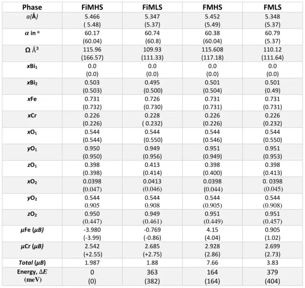
spin-polarized calculations and complete relaxation. The results revealed small differences with what has been reported in literature. The differences are chiefly in the contribution of Fe and Cr to the total magnetic moment, the energy of the fully optimized structure, as well as the position of some ions. The total magnetic moment per unit cell of the ferrimagnetic high spin (FiMHS) and ferromagnetic high spin (FMHS) configurations are 1.987 μB and 7.66 μB, respectively, while that of the ferrimagnetic low spin (FiMLS)

and ferromagnetic low spin (FMLS) configurations results in values of 3.8 μB and 1.88 μB,

respectively. For completeness, the ionic charges, as well as the density of state have been calculated. Despite slight differences, our results are in overall agreement with what has been reported in the literature.

Secondly, we have investigated the effect of the epitaxial strain on the electronic and magnetic properties of the BFCO system. To this end, the lattice parameters of the rhombohedral BFCO unit cell have been fixed to the STO parameters in the plane of the BFCO/STO interface and the out-of-plane lattice parameter has been varied. We found that FiMHS remains the ground state configuration of the BFCO system under the epitaxial constraint of STO. The influence of the epitaxial deformation imposed by the STO substrate mainly manifests itself in the ionic contribution to spontaneous polarization by inducing a change of 7.64 μC cm-2 _{for the the ground state (FiMHS), and}

in the unstrained case. The magnetic moments of the constrained and unconstrained BFCO are very similar, the main difference being observed for the FiMLS phase, with 1.905 μB instead of 1.880 μB. Finally, we have calculated the density of states. Comparing

with the case of the system without constraint, we found that the band gap remains practically unchanged for FiMHS, is reduced by 0.1 eV (-10%) for FMHS, and almost vanishes for FMLS and FiMLS.

Acknowledgement

Firstly, I would like to express my sincere gratitude to my supervisor Professor Alain Pignolet for his guidance, great support, and precious advices. I am especially thankful for the freedom he gave me to do this work.

I owe my deepest and honest thanks to my co-supervisor Professor François Vidal for his constant support, infinite patience, and his constructive suggestions which were essential in the development of this work.

I would like to take this opportunity to acknowledge the jury members for agreeing to read and evaluate this work.

There are not enough words to thank the Ph.D. candidate Mohamed Cherif for his support and encouragement.

Special thanks to Dr. Liliana Braescu who offered me insightful discussions and valuable suggestions throughout my research. I am also very grateful to Dr. Luca Corbellini who has been helpful in providing advice many times during.

Finally, I would like to thank all those who supported me during this journey: all of my family members and my friends.

Table of Contents

Acknowledgment………iii List oftables………...vii List of figures………viii List of abbreviation………...ix Introduction………..1 References………4

Chapter 1: Density Functional Theory……….6

1.1 Background………6

1.2 Schrödinger’s Equation for many body systems………...7

1.2.1 Born - Oppenheimer approximation (BOA)………...………….8

1.3 Thomas-Fermi model (TF)……….9

1.4 Hohenberg-Kohn Theorem (H-K theorem)………...…...………...10

1.5 Kohn-Sham Equations (KS)………..………...11

1.6 Local Density Approximation (LDA)………...………...14

1.6.1 Local Spin Density Approximation (LSDA)………..……...15

1.7 LDA plus Hubbard model (LDA+U)………...……….15

1.8 References………18

2.0 Introduction...19

2.1 The Perovskite structure...21

2.1.1 Single perovskites………...…………...21

2.1.2 Double perovskites………...……….22

2.2 Deviation from ideality and octahedral rotation………..……...23

2.2.1 Jahn-Teller effect (JT)………...24

2.3 Ferroic materials………...………....26

2.4 Ferroelectric materials………...………...27

2.5 Magnetic materials………...………....30

2.5.1 Diamagnetic and paramagnetic materials………...……...32

2.5.2 Ferromagnetic materials………32

2.5.3 Ferrimagnetism and Anti-ferromagnetism………33

2.6 Multiferroic materials...34

2.7 Magnetoelectric effect……….……….37

2.7.1 Direct and Inverse Magnetoelectric Effect………..………….38

2.7.2 Indirect or Elastically-mediated Magnetoelectric Effect………..39

2.8 Potential applications………...39

2.9 References………40

Chapter 3: Computational Details and Results………...…………..43

3.1 Vienna Ab Initio Simulation Package (VASP)………...………….43

3.2 Introduction to Bi2FeCrO6 (BFCO) crystal structure………...……...44

3.3 Calculations for unstrained BFCO………...………....46

3.3.1 Computing atomic charges………...49

3.4.1 SrTiO3 (STO) crystal structure………..50

3.4.2 Technical details………...…….51

3.5 Variation of the energy as a function of the out-of plane-cell size………….………....51

3.6 Calculations of the Electric Polarization………...58

3.7 Density of state (DOS) calculations for strained and unstrained BFCO……….……...62

3.8 References………66

LIST OF THE TABLES

Table 3.1 Summary of the electronic properties of the unstrained BFCO………...48

Table 3.2 The total charge of each ion in units of the elementary charge………...49

Table 3.3 Calculated parameters and properties of strained BFCO………..…….56

Table 3.4 Total charge of each ion in unit of the elementary charge………..………….57

Table 3.5 Contribution of each ion to ionic polarization...………..………....60

Table 3.6 Polarization results of strained and unstrained BFCO………..…...61

LIST OF FIGURES

Figure 2.1:

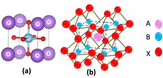
(a) Ideal perovskite structure of formula ABX3 (b Alternate) representations of perovskite

with the BO6 octahedra at the corner of a cube and the large cation A in the

middle………21

Figure 2.2:

Ideal cubic double perovskite of formula A2BB’O6...22

Figure 2.3:

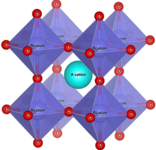
Schematic representation for an ideal perovskite cubic structure………23

Figure 2.4:

Jahn-Teller effect on octahedral copper (II) complex where the green atom represents Cu+2 and red atoms are usually oxygen………..………...25

Figure 2.5:

Hysteresis loop characteristic of a ferroelectric material, showing polarization P as a function of the applied electric field E ………..……….28

Figure 2.6:

Schematic potential well (Gibbs free energy G vs. Polarization P) of a ferroelectric system with first order phase transition for T>Tc, T=Tc, and T<Tc. the red arrows

indicate the polarization states ………...29

Figure 2.7:

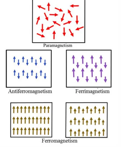
Classification of magnetic materials according to their magnetic dipole ordering..30

Figure 2.8:

Magnetic hysteresis curve of ferromagnetic material and evolution of the

macroscopic magnetization M as a function of magnetic field H……….33

Figure 2.9:

Schematics representation multiferroics (green color) combining the properties of ferroelctrics (Blue color) and of magnetic materials (yellow color) , i.e. exhibiting both magnetic and ferroelectric hysteresis loops………...35

Figure 3.1:

BFCO rhombohedral structure and ordering of the transition metals Cr and Fe along the <111> direction. 𝒂𝐁𝐅𝐂𝐎_𝐑 , Indicates the lattice constant of the

rhombohedron. 10 atoms of the unit cell are indentified

(Bi1,Bi2,Cr,Fe,O1,…O6)……….44

Figure 3.2:

Crystal field splitting diagram for Fe+3 and Cr+3 with spin orientations in the high-spin and low-high-spin cases………..45

Figure 3.3:

Cubic structure of STO with lattice constant = 3.905 Å…...………...51

Figure 3.4:

Sketch of the rhombohedra in a hilghly symmetric cubic BFCO…..………53

Figure 3.5:

Modifying BFCO lattice constant ( 𝑎⃗_BFCOR) to fit exactly STO lattice constant

(𝑎𝑆𝑇𝑂) ………53

Figure 3.6:

The relation between the energy and f. The total magnetic moment per unit cell and the quality of the fits by quartic polynomials are also shown……….54

Figure 3.7:

Energy vs. f for the four phases of BFCO (FIMLS, FMLS, FMHS, and FIMHS) and of the fit of quartic polynomials………..55

Figure 3.8:

Projected DOS of the FIMHS and FMHS phases of strained BFCO (left) and unstrained BFCO (right). Spins up and down are represented on the positive and negative vertical axis, respectively. The DOS calculations are performed with U = 3 eV and J = 0.8 eV………...64

Figure 3.9:

Projected DOS of the FIMLS and FMLS phases of strained BFCO (left) and unstrained BFCO (right). Spins up and down are represented on the positive and negative vertical axis, respectively. The DOS calculations are performed with U = 3 eV and J = 0.8 eV………...65

Figure 4.1:

Supercell represents BFCO thin film containing three layers of BFCO and two layers of STO as a substrate………...68

LIST OF ABBREVIATIONS

BFCO Bi2FeCrO6 DFT Density functional theory

STO SrTiO3

LSDA+U Local spin density approximation plus Hubbard model

VASP Vienna Ab Initio Simulation Package FiMHS Ferrimagnetic high spin

FMHS Ferromagnetic high spin FiMLS Ferrimagnetic low spin

FMLS Ferromagnetic low spin

DOS Density of states BFMO Bi2FeMnO6 BNMO Bi2NiMnO6 BFO BiFeO3 BCO BiCrO3 TF Thomas-Fermi HF Hartree-Fock

BOA Born-Oppenheimer approximation

LDA Local density approximation

PLD Pulsed laser deposition

JT Jahn-Teller (effect)

PAW Projector augmented wave (method)

BZK Brillouin zone k-points

RWIG Wigner –Seitz Radius

CFT Crystal Field Theory

LAO LaAlO3

Introduction

Nowadays, the ongoing development of theories leading to the design of numerical algorithms and of electronic structure software packages has enabled the study of quite complicated physical systems with high reliability and in a reasonable time. Ab initio density functional theory (DFT), which is built on the first principles of quantum mechanics, has proven to be an astonishing tool, very successful in material science as well as in other fields. The DFT formalism relies on the electron density, instead on the wave function, in order to determine the ground state properties of a system of electrons without the need of empirical adjustable parameters.

DFT has been widely used to investigate the properties of interest in many materials. As such, it has also been among the techniques used to predict the properties of a family of materials called multiferroics. The formal definition of a multiferroic material is the simultaneous presence of more than one ferroic order in the same phase. In most cases, multiferroic materials show a ferroelectric order (often accompanied by a ferroelastic order) and a ferromagnetic or antiferromagnetic order [1]_{. Such a multiplicity of} physiochemical properties in a single material, with promising potential applications (such as controlling the magnetic properties of the multiferroic material electrically), has attracted a significant attention. Therefore, theoretical and experimental studies are currently being dedicated to gain fundamental understanding of the magnetic and electric properties of single-phase multiferroic crystals. The valuable properties of multiferroics are mainly related to the presence of the magnetoelectric effect (interplay between electrical polarization and magnetization), which gives these materials their great significance in terms of the variety of applications they could potentially enable, particularly in electronic devices. Several bismuth-based double perovskites of the Bi2BB’O6 family, such as Bi2FeCrO6 (BFCO), Bi2FeMnO6 (BFMO), and Bi2NiMnO6

(BNMO) are promising candidates exhibiting multiferroism [2] [3] [4]_.

BFCO was designed by combining its parents, the Bi-based BiFeO3 (BFO) and BiCrO3

(BCO) in a unit cell. BFCO has attracted intensive attention in particular after the experimental observation of multiferroicity at room temperature exceeding the properties

predicted by DFT calculations [5]_{. The first DFT calculations to investigate BFCO} properties were done by Baettig et al., and they reported that the lowest energy structure belongs to the R3 symmetry group with a rhombohedral distorted unit cell, with 𝑎𝑟ℎ =

5.47 Å and 𝛼𝑟ℎ= 60.09o. The B-site of the rhombohedral structure is occupied by alternate

Fe3+ _{and Cr}3+ _{ions with a perfect ordering along the (111) direction. Ferromagnetism and}

insulating properties stem from superexchange interaction of the spatial spin arrangement of Fe-d5 _{and Cr-d}3 _{cations, while the ferroelectricity is attributed to the Bi}3+

with the stereochemically active 6s2 _{lone pair of electrons. An estimation of the magnetic}

Curie temperature of the BFCO system was provided by calculating the exchange coupling constant of nearest neighbors through the mean-field approximation. Baettig et al. work clearly highlighted promising multiferroic properties with electric polarization of 80 μC. cm−2 _{and magnetic moment of 2 μ}

B per formula unit (f.u.) for the ferrimagnetic

ground state configuration of BFCO [6][7]_{. Since then, the experimental efforts relied on} thin film deposition techniques, whereby strain engineering is used to enhance the multifunctional properties of BFCO epitaxial thin films. The growth of BFCO thin film was successfully obtained on SrTiO3 (STO) substrate with a measured magnetic moment

of 1.91 μB/f. u. and a remenant polarization of 60 μC. cm−2[5]. These experimental findings

are consistent with the DFT calculation of Ref. [6]_{, although those calculations were done} at 0 K while the ferroelectric and magnetic measurements were performed at room temperature. Calculations of Ref. [9]_{, performed using advanced computational} techniques, predicted a Curie temperature of ~450 K. It has been recognized that the properties of materials with a perovskite structure, in particular those with a double-perovskite structure, are strongly sensitive to the influence of epitaxial strain [10]_. Epitaxial strain is commonly used experimentally to control the thin film properties, and it can be simulated theoretically. When a thin film (single crystal) grows on the top of a crystalline substrate, it keeps the symmetry of the crystallographic plane forming the substrate surface and also tries to keep the lattice constants of this plane, and the overlayer is said to have grown epitaxially. The crystallographic structure of the monocrystalline overlayer thus depends on the arrangement of the atoms in the substrate as well as on it crystallographic orientation. For the case of the growth of BFCO film on STO, the structure of the film is deformed due to slightly different lattice parameters

(lattice mismatch) of the two materials. Hence, in heteroepitaxy (growth of a film of a different material than the substrate), the effects of strain are unavoidable and can influence significantly the physical properties of the investigated epitaxial thin films. The progress in materials modeling opens the possibility to simulate the experimentally observed strain effects. Epitaxial strain can be implemented in DFT calculations by fixing the in-plane lattice parameters (a and b) which are related to the substrate, whereas relaxation of the remaining structural parameters is permitted in accord with the global energy minimum under epitaxial constraint [7]_{. In this regard, the influence of epitaxial} strain on several Bi-based perovskite structures have been investigated. Unstrained bismuth ferrite BFO exhibits a polarization of 96 μC cm−2 _{with a very weak net}

ferromagnetic moment, whereas epitaxial strain calculations predicted a high intrinsic polarization up to 150 μC. cm−2 _{when the tetragonal BFO structure is strongly elongated}

out of the plane [10]_{. This predicted giant ferroelectricity was indeed experimentally}

observed [11]_{. Double perovskite BFMO is another single-phase multiferroic candidate} that has been investigated theoretically and experimentally demonstrated. Recently, experimental measurements at room temperature reported that BFMO-strained thin films have a magnetization value of 1.16 μB/f. u. [12]. The stable sate of the fully relaxed

BFMO thick film predicted from non-magnetic DFT calculations has a monoclinic symmetry. In addition, a self-consistent calculation carried out on strained tetragonal BFMO predicted that the total magnetic moment depends on epitaxial strain: for a particular c/a ratio of 1.27, the total magnetic moment was found to be 1.11 μ_B/f. u. while for c/a = 1.45 (experimental ratio of BFMO/STO films), the magnetic moment found was 1.05 μB/f. u. [13][14]. Regarding recent work on BFCO, magnetic and electronic properties

were computed by Goffinet et al. within the DFT framework [15]_{. Four possible magnetic} configurations were examined for 4 cases of spin ordering, namely FiMLS, FiMHS, FMLS and FMHS, i.e. an antiparallel spin arrangement (ferrimagnetic – FI) and a parallel spin arrangement (ferromagnetic – FM), for both high spin (HS) and low spin (LS) configurations of iron. The results showed that the FiMHS configuration represents the ground state of the BFCO system with a magnetic moment of 2 μB per unit cell (in

agreement with previous works), while the FMHS is predicted to have a slightly higher energy than the ground state. They found that reducing the volume of the unit cell leads

to a crossover between FiMLS and FiMHS as the lowest energy state (however, both states have the same magnetic moment of 2 μB). More recently, DFT was employed in order to

investigate the influence of epitaxial strain on BFCO by using a tetragonal supercell involving 20 atoms. Interestingly, a magnetic moment of 2 μB/f. u. was reported [16].

The main objectives of this work are to investigate the properties of epitaxially strained rhombohedral BFCO on a STO substrate within the framework of DFT calculations in order to compare the obtained results with those obtained for unstrained BFCO. As we mentioned previously, it is expected that BFCO properties are affected by the epitaxial strain and, toward this end, we imposed the value of the STO lattice parameter to the pseudo-cubic lattice parameter of rhombohedral BFCO in order to simulate the strained BFCO epitaxial thin film. In the simulation, we fixed the in-plane parameters and varied manually the out-of-plane parameter of the unit cell. We performed full relaxation within these constraints. In contrast, all the structural parameters of unstrained BFCO are fully relaxed. Electric and magnetic properties were investigated in both cases. At the end, we come up with a comparison between strained and unstrained BFCO.

References

1. H. Schmid, Ferroelectrics, 162,317 (1994)

2. S. Kamba1, D. Nuzhnyy, R. Nechache, K. Zaveta, D. Niznansky, E. antava, C.Harnagea, and A. Pignolet, Phys. Rev. B 77, 104111 (2008)

3. Lei Bi, A. R. Taussig, Hyun-Suk Kim, Lei Wang, G. F. Dionne, D. Bono, K. Persson, G. Ceder, and C. A. Ross, Phys. Rev. B 78, 104106 (2008)

4. M. N. Iliev, P. Padhan, and A. Gupta, Phys. Rev. B 77, 172303 (2008)

5. R .Nechache, C. Harnagea, L. P. Carignan, et al, J. Appl. Phys. 105, 061621 (2009) 6. P. Baettig, C. Ederer, N.A. Spaldin, Phys. Rev. B 72, 214105 (2005)

7. P. Baettig, N.A. Spaldin, Appl. Phys. Lett. , 86, 012505 (2005)

8. S. Picozziand, C. Ederer, J. Phys.: Condens. Matter, 21 303201 (2009) 9. Song Zhe-Wen, Liu Bang-Gui, Chin. Phys. B Vol. 22, No. 4, 047506 (2013) 10. A. J. Hatt, N. A. Spaldin, C. Ederer, Phys. Rev. B 81, 054109 (2010)

12. L. Bi, A. R. Taussig, H.-S. Kim, L. Wang, G. F. Dionne, D. Bono, K. Persson, G. Ceder, and C. A. Ross, Phys. Rev. B 78,104106 (2008)

13. T.Ahmed, A.Chen, D. A. Yarotski, S. A. Trugman, Q. Jia, and Jian-Xin Zhu, APL Materials 5, 035601 (2017)

14. M. Goffinet, J. Iniguez, and P. Ghosez, Phys. Rev. B 86, 024415 (2012) 15. P. C. Rout, A. Putatunda, and V. Srinivasan, Phys. Rev. B 93, 104415, (2016)

Chapter 1. DENSITY FUNCTIONAL THEORY

1.1 Background

The first vision of density functional theory (DFT) started from Thomas and Fermi (TF) in 1920. The TF model was designed to calculate the electron distribution inside the atom. In 1928, Dirac improved the TF work by adding exchange energy density. However, the theory of Thomas-Fermi-Dirac was inaccurate for most applications due to the weak representation of the kinetic energy as a function of the electron density and to the absence of electron correlation in the model. Ab initio (first principles) methods with various approximations and assumptions have been developed to study the properties of many-body-systems [1]_{. The Hartree-Fock (HF) method is the simplest ab initio method}

for treating interacting systems. This method assumes that the electron can affect the average potential created by the other electrons. In fact, considerable complications occur due to considering single electron orbitals and solving many wave functions. The difficulty of using HF calculations increases as the number of electrons goes up[2]_.

In 1964, Hohenberg and Kohn introduced the bases of DFT. Their main idea was to determine the electronic ground state energy of the system from the electron density. According to their work, the electron density of the ground state not only uniquely determines the total energy of the ground state but also all the other system’s properties. Since the electron density is a single three-dimensional distribution in space, there is no need to calculate the wave function of each electron in the system as in the HF method. In order to specify the energy of the ground state corresponding to the electron density, it is necessary to formulate a functional relating these two quantities.

The year after, Kohn and Sham introduced the exchange correlation functional, which relates the electron density to the ground state energy. The Kohn-Sham method is a mathematical model based on a non-interacting electrons system. In their approximated approach, the exchange correlation functional takes into account the quantum interaction between electrons [3].

The main objective of this chapter is to introduce the basics of DFT, starting from the resolution of the non-relativistic Schrödinger’s equation.

1.2

Schrödinger’s Equation for Many Body Systems

Resolving the Schrödinger’s equation for many body systems has been attempted since quantum mechanics emerged. Analytically, obtaining the exact solution for a system having more than two electrons is however impossible [4]_{. In quantum mechanics, all the} observable quantities can be obtained from the system’s wave function Ψ. In a stationary system, this wave function is calculated from the non-relativistic time-independent Schrödinger’s equation, which for a distribution of electrons and nuclei can be written generally as

{𝐻 − 𝐸}Ψ(𝑟, 𝑅) = 0 (1.1) where E is the total energy of the system and the Hamiltonian given by

𝐻 = 𝑇 + 𝑉_𝑒−𝑒 + 𝑉_𝑒−𝑛+ 𝑉_𝑛−𝑛 (1.2) Here r and R represent collectively the positions of the electrons and of the nuclei, respectively. In Eq. (1.2), T is the kinetic energy of the electrons and nuclei, 𝑉𝑒−𝑒 is the

potential energy due to electron-electron interaction, 𝑉𝑒−𝑛 is the potential energy of the

electron-nuclei interaction, and 𝑉𝑛−𝑛 is the nuclei-nuclei interaction. The wave function

Ψ(𝑟, 𝑅) depends on the positions and spin coordinates of all N nuclei and n electrons in the system.

In the following we use the atomic units ℏ = 𝑒 = 4𝜋𝜖0= 𝑚𝑒 = 1. For a normalized

distribution of electrons with coordinates 𝑟𝑖 and nuclei with charges 𝑍𝑎 and

coordinates 𝑅𝑎, the terms of Eq. (1.2) can be written (ignoring the spin and

spin-orbit interactions here for simplicity),

𝑇 = −1₂{∑ ∇_{𝜇 𝜇}2+ ∑ 1 𝑀𝑎 𝑎 ∇𝑎2}; 𝑉𝑒−𝑒 = + 1 2∑ 1 ⃓𝐫𝜇−𝐫𝑣⃓ 𝜇,𝑣(𝜇≠𝑣) ; 𝑉_𝑒−𝑛 = − ∑ 𝑍𝑎 ⃓𝐫𝜇−𝐑𝑎⃓ 𝜇,𝑎 ; 𝑉𝑛−𝑛 = + 1 2 ∑ 𝑍𝑎𝑍𝑏 ⃓𝐑𝑎−𝐑𝑏 𝑎,𝑏(𝑎≠𝑏) ;

The kinetic energy T involves a sum over all electrons (𝜇 = 1 → 𝑛) and nuclei (α = 1→ 𝑁 ). The electron-electron and nuclei-nuclei potentials are the sum over all combinations of distinct pairs. To avoid each pair from being counted twice, the potentials 𝑉𝑒−𝑒 and 𝑉𝑛−𝑛

are multiplied by 𝟏

𝟐 .

1.2.1 Born - Oppenheimer approximation (BOA)

The BOA is a simplification that has been used almost in all methods to solve Schrödinger’s equation for atomic systems. It is well known that the charge magnitude is the same for electrons and protons while the mass ratio of electron to the proton is 1/1836. Since the mass of the nuclei is much greater than the electron’s mass, electrons can move much faster than the nuclei. Hence, the electron distribution will change rapidly with the variation of the nuclei field [5]_{. Therefore, it is possible to consider the position of the} nuclei R as fixed relative to the electrons motion. Accordingly, BOA allows to decouple the total wavefunction into the electronic part and nuclear part. This is also called the adiabatic approximation. In this way, the total wave function for fixed nuclear arrangement, Ψ(𝑟, 𝑅), can be expressed as an expansion over the set of adiabatic electron wavefunctions 𝜑_𝑘(𝑟, 𝑅):

Ψ(𝐫, 𝐑) = ∑ 𝜒𝑘 𝑘(𝐑)𝜑𝑘(𝐫, 𝐑) (1.3)

where 𝜒𝑘(𝐑) is the expansion coefficients depending only on the parameter R.

The 𝜑𝑘(𝐫, 𝐑) 𝑠atisfy the following wave equation for electrons:

{−1

2∑ ∇𝜇 2

𝜇 + 𝑉𝑒−𝑒+ 𝑉𝑒−𝑛+ 𝑉𝑛−𝑛} 𝜑𝑘(𝐫, 𝐑) = 𝐸𝑘(𝐑)𝜑𝑘(𝐫, 𝐑) (1.4)

where we assumed that the kinetic energy of the nuclei is zero.

In order to obtain the nuclear wave function, we write the full Schrödinger Eq. (1.1) as {−1₂ ∑ 1

𝑀𝑛

𝑛 ∇𝑛2 + 𝐻𝑒} Ψ(𝐫, 𝐑) = 𝐸Ψ(𝐫, 𝐑) (1.5)

Where He is the electron Hamiltonian expressed by the terms in brackets in Eq. (1.4) (by

∑ 𝜑𝑘(𝐫, 𝐑) {− 1 2∑ 1 𝑀𝑛 𝑛 ∇𝑛2 + 𝐸𝑘(𝐑) − 𝐸} 𝜒𝑘(𝐑) 𝑘 = ∑ ∑ 1 2𝑀𝑛 𝑛 {𝜒𝑘(𝐑)∇𝑛2𝜑𝑘(𝐫, 𝐑) + 𝑘 2∇𝑛𝜒𝑘(𝐑)· ∇𝑛𝜑𝑘(𝐫, 𝐑) (1.6)

which is decoupled from the electronic movement. Considering Eq. (1.6) together with Eq. (1.4), one sees that the description of the nuclear and electronic movements can be made separately [6]_.

1.3 Thomas –Fermi (TF) Model

Thomas and Fermi considered an ideal system relying on the kinetic energy of non-interacting electrons. The TF model approximates the electron distribution in the atom as a homogeneous gas [7]_{. If electrons behave as independent fermionic particles at zero} Kelvin, the energy levels of the electrons in cubic potential well are given by

𝐸( 𝑛𝑥 , 𝑛𝑦 , 𝑛𝑧) = 𝜋2 2𝑙2 ( 𝑛𝑥 2_{+ 𝑛} 𝑦 2 _{+ 𝑛} 𝑧 2 _{) (1.7)}

where 𝑛𝑥 , 𝑛𝑦 , 𝑛𝑧 are integer numbers and l is the length of the cubic edge.

The Fermi energy corresponds to the highest energy level for N electrons in a volume 𝑉 = 𝑙3_{, respecting the Pauli principle, and is given by:}

𝜖𝐹(𝜌) = 1 2(3𝜋

2_𝜌)2/3 _(1.8)

where 𝜌 = 𝑁/𝑉 is the electron density. For this electron density, the kinetic energy density is given by ∫ 𝜖₀𝜌 _𝐹(𝜌′)𝑑𝜌′ =3 5𝜖𝐹(𝜌)𝜌 = 𝐶𝐹𝜌 5/3 _(1.9) where 𝐶𝐹 = 3 10( 3 8𝜋) 2/3 .

The total energy of a system, submitted to an external potential 𝑉𝑒𝑥𝑡(𝒓), thus depends only

on the electron density ρ and is given by the sum of the kinetic and potential energies 𝐸_𝑇𝐹 [𝜌] = 𝐶_𝐹∫[𝜌(𝐫) ]5⁄3_{𝑑𝐫 + ∫ 𝜌(𝐫) 𝑉𝑒𝑥𝑡}(𝐫)𝑑𝐫 + ∫ ∫𝜌(𝐫)𝜌(𝐫

′₎

Eq. (1.10) shows that the electron density can be used instead of the wavefunction to describe the total energy of the electronic system.

The TF model is accurate only if the system consists of one atom. Although the TF model fails to describe large systems, it is considered as the starting point to DFT (Hohenberg and Kohn theorem) [8]_.

1.4 Hohenberg-Kohn Theorem (H-K theorem)

The first H-K theorem states that for systems containing N electrons in an external potential V(r) (Coulomb potential usually generated by the nuclei), the external potential

V(r) is completely determined by the electron density 𝜌(𝒓) associated with the ground

state energy [9]_.

To prove that, consider the Hamiltonian of a many-body system: 𝐻 = − ∑𝑁 1₂

𝑖=1 ∇𝑖2+ ∑𝑁𝑖<𝑗 𝑈(𝐫𝑖 , 𝐫𝑗) + ∑𝑁𝑖=1 𝑉(𝐫𝑖) ≡ 𝑇 + 𝑈 + 𝑉 (1.11)

where T is the kinetic energy, U the energy of electron-electron interaction, and V is the external potential. The electron density is defined as

𝜌(𝐫) = 𝑁 ∫|𝛹(𝐫, 𝐫2, … , 𝐫𝑁)|2𝑑𝐫2… … . 𝑑𝐫𝑁 (1.12)

where Ψ is the electron wave function. Consider now a Hamiltonian 𝐻′ _{= 𝑇 + 𝑈 + 𝑉}′

where 𝑉 − 𝑉′ _{≠ 𝑐𝑜𝑛𝑠𝑡. The wave function of the ground state for 𝐻}′ _{is Ψ}′_{. Then we have}

the following inequality:

𝐸′_{= ⟨Ψ}′_|𝐻′_|Ψ′_{⟩ < ⟨Ψ|𝐻}′_{|Ψ⟩ (1.13)}

where

⟨Ψ|𝐻′_{|Ψ⟩ = ⟨Ψ|𝑇 + 𝑈 + 𝑉 + 𝑉}′_{− 𝑉|Ψ⟩}

= 𝐸 + ⟨Ψ|𝑉′_{− 𝑉|Ψ⟩}

Now, assume that the electron density ρ(r) is the same for both 𝐻 and 𝐻′_{. Then a similar}

inequality must hold when inverting the prime and nonprime quantities: 𝐸 < 𝐸′_{+ ∫ 𝜌(𝐫)[𝑉(𝐫) − 𝑉}′_{(𝐫)]𝑑𝐫}

Adding up the last two inequalities, one finds 𝐸′_{+ 𝐸 < 𝐸 + 𝐸′. This contradiction implies}

the impossibility of associating the same electron density ρ(r) to both external potentials 𝑉(𝒓) and 𝑉′(𝒓). Therefore, the external potential is uniquely determined by the electron density ρ(r), as stated in the first H-K theorem.

The second H-K theorem states that the ground state energy can be obtained from a variational principle, i.e. the density that minimises the total energy is the exact ground state density. The proof is also straightforward. We can represent the energy as the functional

𝐸[𝜌(𝐫)] = ⟨Ψ|𝑇 + 𝑈|Ψ⟩ + ⟨Ψ|𝑉|Ψ⟩ = 𝐹[𝜌(𝐫)] + ∫ 𝜌(𝐫)𝑉(𝐫)𝑑𝐫 (1.14) where 𝐹[𝜌(𝐫)] is a universal functional depending only on the electron density ρ(r). The variational principle states that:

⟨Ψ′_{|𝑇 + 𝑈 + 𝑉|Ψ}′_{⟩ > ⟨Ψ|𝑇 + 𝑈 + 𝑉|Ψ⟩}

We thus obtain:

𝐸[𝜌′_{(𝐫)] > 𝐸[𝜌(𝐫)]}

which implies that the density that minimises the total energy is the exact ground state density and proves the theorem.

1.5 Kohn-Sham (KS) Equations

Since the kinetic energy of the system of interacting electrons is unknown, Kohn and Sham proposed to replace the system of interacting electrons by a system of non-interacting electrons evolving in an effective potential, imposing that the electron density in the ground state is the same for both systems [10][11]_{. This amounts to replace the} Hohenberg-Kohn functional (1.14)

𝐸_𝐻𝑆[𝜌] = 𝐹[𝜌] + ∫ 𝜌(𝐫)𝑉(𝐫)𝑑𝐫 by the following one

𝐸𝐾𝑆[𝜌] = 𝑇𝐾𝑆[𝜌] + 𝐽[𝜌] (1.15)

where is 𝑇𝐾𝑆[𝜌] is the non-interacting kinetic energy and

𝐽[𝜌] = 𝑉 + 𝑈 + (𝑇 − 𝑇𝐾𝑆) Therefore: 𝐸_𝐾𝑆[𝜌(𝐫)] = − ∑ ⟨Ψ_𝑖|1 2∇𝑖 2_|Ψ 𝑖⟩ 𝑖 + 1 2 ∫ ∫ 𝜌(𝐫)𝜌(𝐫′) |𝐫−𝐫′_| 𝑑𝐫𝑑𝐫′ + 𝐸𝑋𝐶[𝜌(𝐫)] + ∫ 𝜌(𝐫)𝑉(𝐫) 𝑑𝐫 where the Ψ𝑖 form a set of functions (called orbitals) so that

𝜌(𝐫) = ∑ 𝑓_𝑖|Ψ_𝑖(𝐫)|2

𝑖

where fi is the number of electrons in the orbital i (normally fi = 2).

In 𝐸_𝐾𝑆[𝜌], the first term is the kinetic energy and the second term is the Hartree term that takes into account the repulsion of the electron cloud. The term 𝐸𝑋𝐶[𝜌] is the

exchange-correlation term, which represents everything that is not taken into account by the other terms. The exchange term is a quantum mechanical effect producing a pseudo force between electrons that results from their undistinguishable nature. The correlation term describes the departure from the non-interacting electron assumption.

The orbital functions Ψ_𝑖 are obtained by minimizing the energy 𝐸_𝐾𝑆[𝜌] under the orthonormal constraints ∫ Ψ_𝑖∗_{(𝐫) Ψ}

𝑗 (𝒓)𝑑𝐫 = 〈Ψ𝑖| Ψ𝑗〉 = 𝛿𝑖𝑗. This is done using the

variational method of Lagrange multipliers

𝛿{𝐸[𝜌(𝑟)] − ∑ 𝜆_{𝑖𝑗 𝑖𝑗} (∫ Ψ𝑖∗(𝒓) Ψ𝑗(𝒓)𝑑𝒓 − 𝛿𝑖𝑗)} = 0 (1.16)

where the operator 𝛿 denotes an arbitrary variation of Ψ𝑖. In this expression, the 𝜆𝑖𝑗 are

the Lagrange multipliers such that 𝜆𝑖𝑗 = 𝛿𝑖𝑗𝜖𝑗 due to the orthonormality condition of the

Ψ_𝑖. One thus has to solve the following variation equation for 𝜌(𝒓) :

𝛿{𝐸[𝜌(𝐫)] − ∑ 𝜖𝑖 𝑖 ∫ Ψ𝑖∗(𝐫)Ψ𝑖(𝐫) 𝑑𝐫 } = 0 (1.17)

𝛿 ∑ ∫ Ψ_𝑖∗ 𝑖 (𝐫)∇_𝑖2_Ψ 𝑖(𝐫) 𝑑𝐫 = 2Re [∑ ∫ 𝛿Ψ𝑖∗(𝐫)∇𝑖2 𝑖 Ψ_𝑖(𝐫)]

where Re denotes the real part of the argument. Furthermore, 𝛿 ∑ ∫ Ψ_𝑖∗ 𝑖𝑗 (𝐫)Ψ_𝑖(𝐫) 1 |𝐫 − 𝐫′_| Ψ𝑗 ∗_(𝐫′_)Ψ 𝑗 (𝐫′)𝑑𝐫 𝑑𝐫′ = 4Re [∑ ∫ 𝛿Ψ_𝑖∗ 𝑖𝑗 (𝐫)Ψ𝑖(𝐫) 1 |𝐫 − 𝐫′_|Ψ𝑗∗(𝐫′)Ψ𝑗 (𝐫′)𝑑𝐫 𝑑𝐫′] In addition, 𝛿 ∑ ∫ Ψ_𝑖∗ 𝑖 (𝐫)Ψ𝑖(𝐫)𝑉(𝐫)𝑑𝐫 = 2Re [∑ ∫ 𝛿Ψ𝑖∗ 𝑖 (𝐫)Ψ𝑖(𝐫)𝑉(𝐫)𝑑𝐫] and, 𝛿𝐸_𝑋𝑐[𝜌(𝐫)] = 𝛿𝐸𝑋𝑐 𝛿𝜌(𝐫) 𝛿 ∑ Ψ𝑖 ∗ 𝑖 (𝐫)Ψ_𝑖(𝐫) = 𝛿𝐸𝑋𝐶 𝛿𝜌(𝐫) 2Re [∑ 𝛿Ψ𝑖 ∗ 𝑖 (𝐫)Ψ_𝑖(𝐫)]

Eq. (1.17) thus becomes

∑{∫ 𝛿Ψ_𝑖∗(𝐫)[−1 2 𝑖 ∇_𝑖2+ ∑ ∫ Ψ_𝑗∗ 𝑗 (𝐫′) 1 |𝐫 − 𝐫′_|Ψ𝑗(𝐫′)𝑑𝐫′+ 𝛿𝐸𝑋𝐶 𝛿𝜌(𝐫) + 𝑉(𝐫) − 𝜖_𝑖 ]Ψ_𝑖(𝐫)𝑑𝐫} = 0 This is satisfied for an arbitrary variation 𝛿Ψ𝑖∗ only if

[−1 2∇𝑖 2_{+ 𝑉} 𝐾𝑆 (𝐫)]Ψ𝑖(𝐫) = 𝜖𝑖Ψ𝑖(𝐫) (1.18) where 𝑉𝐾𝑆 (𝐫) = ∫ 𝜌(𝐫′) |𝐫−𝐫′_|𝑑𝐫 ′₊𝛿𝐸𝑋𝐶 𝛿𝜌(𝐫)+ 𝑉(𝐫) (1.19)

is the K-S potential. The total energy is given by 𝐸 = ∑ 𝜖𝑖 𝑖 + 𝐸𝑋𝐶− ∫

𝜌(𝐫)𝜌(𝐫′₎

|𝐫−𝐫′_| 𝑑𝐫𝑑𝐫

′_{− ∫}𝛿𝐸𝑋𝑐

The K-S Eq. (1.18), is solved in a self-consistent way for the wavefunctions Ψ_𝑖 and their eigenvalues 𝜖𝑖. This consists in starting from an initial guess for 𝜌(𝐫), then to calculate

𝑉_𝐾𝑆(𝐫) and then to solve the Kohn-Sham equation for the Ψ_𝑖(𝐫). Then a new 𝜌(𝐫) is calculated and all the operations are repeated until convergence is obtained.

Although the approach of Kohn and Sham is exact, so far the exchange correlation functional 𝐸𝐾𝑆[𝜌] is unknown, and therefore it is necessary to apply approximations to

this functional. The Local Density Approximation (LDA) discussed in the next section is the simplest approximation.

1.6 Local Density Approximation (LDA)

In the K-S equation the exchange-correlation term 𝛿𝐸𝑋𝐶

𝛿𝜌(𝐫) remains to be determined. Hence,

resolving this difficulty is crucial. Toward this end, a simple approximation was presented by K-S in 1965. This approach is known as LDA for energy exchange and correlation. These authors showed that if 𝜌 varies extremely slowly with position then 𝐸𝑋𝐶 energy can

be expressed by [12][13]

𝐸_𝑋𝑐𝐿𝐷𝐴_{[𝜌] = ∫ 𝜌(𝐫) 𝜀}

𝑋𝐶(𝜌)𝑑𝐫 (1.20)

The potential entering the Kohn-Sham equation associated with this functional is 𝑉_𝑋𝐶𝐿𝐷𝐴= 𝛿𝐸𝑋𝐶𝐿𝐷𝐴

𝛿𝜌 = 𝜀𝑋𝐶(𝜌(𝐫)) + 𝜌(𝐫)

𝜕𝜀𝑋𝐶(𝜌)

𝜕𝜌

In LDA, the functional 𝜀𝑋𝐶(𝜌) is expressed as the exchange energy plus the correlation

energy of a homogeneous electron gas with density𝜌

𝜀_𝑋𝐶(𝜌) = 𝜀_𝑋(𝜌) + 𝜀_𝑐(𝜌) (1.21) The exchange term for a homogeneous electron gas is known analytically to be

𝜀𝑋(𝜌) = − 3 4 ( 3 𝜋) 1 3 ⁄ 𝜌1⁄3. (1.22)

The correlation energy per particle of a homogeneous electron gas 𝜀𝑐(𝜌) is not known

using Quantum Monte Carlo (QMC) methods and then fitted into an analytical form. For example, the simple Chachiyo 2016 fit function [14] _reads

𝜀𝐶(𝜌) = 𝑎 ln (1 + 𝑏 𝑟𝑠+

𝑏

𝑟_𝑆2)

Here a and b are fitting parameters which can also be determined from the known limiting cases.

1.6.1

Local Spin Density Approximation (LSDA

)

For spin-polarized systems, the exchange-correlation functional 𝐸𝑋𝐶 now depends on the

spin up and spin-down density, 𝜌↑ _{and 𝜌}↓_{, respectively. The potentials entering the K-S}

equation for exchange and correlation are now

𝑉_𝑋𝐶↑ = 𝛿𝐸𝑋𝐶[𝜌 ↑_{, 𝜌}↓_] 𝛿𝜌↑ 𝑉_𝑋𝐶↓ = 𝛿𝐸𝑋𝐶[𝜌 ↑_{, 𝜌}↓_] 𝛿𝜌↓

for spin up and spin down, respectively. The exchange term is simply expressed in terms of the spin unpolarised functional as

𝐸𝑋[𝜌↑, 𝜌↓] = 1

2(𝐸𝑋[2𝜌 ↑_{] + 𝐸}

𝑋[2𝜌↓]) (1.24)

For the correlation energy density, it is necessary to introduce a different scheme to approximate the functional. The idea is to start from the energy of the fully polarized homogeneous system and then introduce the relative spin polarization

𝜁 = 𝜌↑−𝜌↓

𝜌↑_+𝜌↓

If 𝜁 = 0 we have the spin-unpolarized case, which means that the electron gas is paramagnetic. If 𝜁 = ±1 the electron gas is fully spin polarized, corresponding to the ferromagnetic case.

Although LDA is widely used, it does not work at all to describe strongly correlated system since it fails at predicting a band gap. For such systems, one has to use the LDA+U approach.

1.7 LDA plus Hubbard model (LDA+U)

Mott insulators are an important class of material whose insulating properties result from strong electron-electron interactions (strongly correlated system) of orbitals d or f. BFCO falls into this category. LDA cannot describe Mott insulators since it is based on a simple one-electron theory. A way to correct the failure of LDA is to take explicitly into account the interaction between d (or f) electrons through a Hubbard-like model, which describes the transition between conducting and insulating systems. In this model, electrons are separated into two systems (for simplicity, we will restrict the discussion to the spin-independent case) [15]

(i) delocalized s and p electrons, which can still be described by using an orbital-independent one-electron potential (LDA);

(ii) localized d or f electrons taking into account Coulomb d-d interaction. In the Hubbard-like model, the corrected LDA functional reads

𝐸𝐿𝐷𝐴+𝑈 = 𝐸𝐿𝐷𝐴+ 𝑈 ∑𝑖≠𝑗𝑛𝑖𝑛𝑗/2 −

𝑈𝑁(𝑁−1)

2 (1.25)

where U is the Coulomb repulsion parameter, ni are the d-orbital occupancies (i.e. the

number of electrons occupying a given d orbital i) and 𝑁 = ∑ 𝑛𝑖.

The second term of Eq. (1.25) takes into account the interactions between electrons in d orbital while the last term is called the double counting term which needs to be subtracted from the second term. The exchange parameter, usually denoted J, which describes the exchange interaction of electrons on neighboring sites as a consequence of the fermionic nature of the electrons, can be incorporated in the corrected LDA functional by replacing

U by Ueff = U – J. In some more accurate formulations, U and J appear in separate terms

[16]_.

Energies of the orbitals are the derivatives of Eq. (1.25) with respect to ni

𝜖_𝑖𝐿𝐷𝐴+𝑈 = 𝜕𝐸𝐿𝐷𝐴+𝑈

𝜕𝑛𝑖 = 𝜖𝑖

𝐿𝐷𝐴_{+ 𝑈 (}1

2− 𝑛𝑖) (1.26)

Case 1: If 𝑛_𝑖 = 0, orbitals are unoccupied and the orbital energy of LDA changes by +U/2. Case 2: If 𝑛𝑖 ≥ 1, then orbitals are occupied and the orbital energy shifts by at least –U/2

The potential entering in the K-S equation, 𝑉𝑖(𝐫) = 𝛿𝐸 𝛿𝑛𝑖(𝐫) = 𝑉𝐿𝐷𝐴(𝐫) + 𝑈 ( 1 2− 𝑛𝑖) (1.27) which is orbital dependent, thus provides a description for lower and upper Hubbard bands with the energy separation between them equal to the Coulomb parameter U.

1.8 References

1. R. M., Dreizler Gross E.K.U. Introduction. In: Density Functional Theory. Springer, Berlin, Heidelberg (1990)

2. D. R. Hartree. Proc. Camb. Philos. Soc., 24, 89 (1927)

3. V. Sahni,The Hohenberg-Kohn Theorems and Kohn-Sham Density Functional Theory. In: Quantal Density Functional Theory. Springer, Berlin, Heidelberg, (2004)

4. K. Capelle , A bird's-eye view of density-functional theory, Brazilian Journal of Physics (2006)

5. M. Born; J. Robert Oppenheimer , Zur Quantentheorie der Molekeln “On the Quantum Theory of Molecules” (1927)

6. http://www.diss.fuberlin.de/diss/servlets/MCRFileNodeServlet/FUDISS_derivate_00000 0012723/Accardi_2012.pdf

7. http://www.math.mcgill.ca/gantumur/math580f12/ThomasFermi.pdf

8. E. H. Lieb, and B. Simon: The Thomas-Fermi theory of atoms, molecules and solids, Adv. in Math 23 (1977)

9. P. Hohenberg and W. Kohn. Phys. Rev., 136:864B (1964) 10. W.Kohn and L.J.Sham. Phys. Rev., 140A:1133 (1965)

11. W. Koch and M. C. Holthausen. A Chemist’s Guide to Density Functional Theory. Wiley, New York, (2000)

12. C. Fiolhais ,F. Nogueira ,M. Marques, A Primer in Density Functional Theory, Springer (2003)

13. Parr, G .Robert; Yang, Weitao, Density-Functional Theory of Atoms and Molecules, Oxford: Oxford University Press (1994)

14. T. Chachiyo, J. Chem. Phys. 145 (2): 021101 (2016)

15. U. von Barth , L. Hedin, J. Phys. C: Solid State Phys (1972)

16. V. I. Anisimov, I. V. Solovyev, M. A. Korotin, M. T. Czyzyk, and G. A. Sawatzky, Phys. Rev. B 48, 16929 (1993)

Chapter 2. FERROIC and MULTIFERROIC MATERIALS

2.0 Introduction

Historically, a magnetoelectric effects have been observed as early as 1888 by Wilhelm Röntgen, who observed that dielectrics moving through an electric field became magnetized [1] _{Then in 1894, and based on symmetry analysis only, Pierre Curie without} using the term ‘multiferroic’ opened this field of investigation in predicting that an electric polarization of a molecule would be obtained by applying an external magnetic field. Conversely, a magnetic moment would be induced by an external electric field [2]_.

In 1926, the terminology “magnetoelectric” (ME) was used for the first time by Debye to describe this phenomenon, and it was then mathematically described in their famous theoretical physics book series by L. D. Landau and E. Lifshitz in 1957, where they showed that, for certain symmetries and magnetic structures, a magnetoelectric response would be observed [3]_{. A few years later, in 1959, according to symmetry considerations, the form} of the linear magnetoelectric effect in anti-ferromagnetic Cr2O3 was predicted by

Dzyaloshinskii [4]_{. A year later, Astrov confirmed this prediction by observing} experimentally that magnetization can be controlled by applying an electric field [5]_. Despite the fact that interest in magentoelectrics persisted over the next 45 years, over 80 magnetoelectric materials being discovered, a renewed surge of interest started again in 2005, together with a renewed interest in multiferroics [6]_.

Despite the mystery surrounding the presence of two ferroic (or more than two) orders in a single phase, a growing interest in these enigmatic materials resurfaced since the terminology of “multiferroic magnetoelectric” materials was introduced by Schmid in 1994 [7]_{. Thereafter, in 2000, Nicola A. Hill explained why ferromagnetic ferroelectric} coexistence is so rare [8]_{. In 2003, a qualitative progress in this field was achieved when} the group of Ramesh was able to obtain a high ferroelectric polarization through growing a single perovskite BiFeO3 epitaxially. The discovery of a magnetoelectric coupling in

Terbium manganites (TbMnO3, TbMn2O5) followed shortly after [9] [10]. In BFCO the Bi+3

to the partially occupied subshell d5 _{and d}3 _{of Fe}+3 _{and Cr}+3_{, respectively} [11]_{. Using} first-principles calculations within the LSDA+U formalism, the lowest energy of BFCO was found to belong to the R3 space group. DFT calculations show that the most stable state of BFCO corresponds to the ferrimagnetic high spin (FIHS) configuration and that changing the volume of the rhombohedral unit cell, while preserving the cell shape, BFCO exhibits a crossover between the ferrimagnetic high-spin and the ferrimagnetic low spin phases, which becomes more energetically favorable at low volumes [13]_{. An estimation of} the magnetic arrangement vs. temperatures of BFCO was obtained by calculating the exchange coupling constant of the nearest neighbors through the mean-field approximation and first-principles calculations [11]_{. It was found not to exceed Néel} temperature TN equals to 100 K.

Experimentaly, epitaxial thin films of BFCO grown on SrTiO3 (STO), synthesized using

pulsed laser deposition (PLD), clearly presented multiferroic properties at room temperature [12]_{. This finding confirmed in part the theoretical predictions of Ref.} [11]_. DFT calculations show the most stable state of BFCO corresponds to the ferrimagnetic high spin configuration and that changing the volume of the unit cell, BFCO exhibits a crossover between two ferrimagnetic phases [13]_.

This chapter contains a short introduction to perovskite structures and a general presentation of ferroic materials. The last part of the chapter is devoted to multiferroic materials and their potential applications.

2.1 The Perovskite Structure

2.1.1 Single Perovskites

The perovskites have a chemical formula ABX3, where A and B are both metallic cations

and X is an anion (usually an oxygen atom). The structure of the perovskites can be described by its unit cell. There are two different ways to describe the ideal high-symmetry cubic perovskite unit cell: (i) The large A atoms are located on the corner of a cube, a smaller B atoms is located in the center of the cube and X atoms (very often oxygen atoms) are located in the center of each face of the cube, so that they form an octahedron with the

B atom in its center, as shown in Figure 2.1a. (ii) Alternately, the unit cell of the perovskite structure can be described with the small B atoms at the corner of a cube, each B atom being surrounded by an octahedron of X atoms, and the large A atom in the center of the cube, as shown in Figure 2.1b [14]_.

Figure 2.1. (a) Ideal perovskite structure of formula ABX3 (b) Alternate representations of perovskite

with the BO6 octahedra at the corner of a cube and the large cation A in the middle.

In the ideal case of a non-polar phase, the single-perovskite structure has a cubic symmetry. Most of the polar phases having a single perovskite structure are distorted in

order to have a polar axis along which the spontaneous polarization can develop, and thus have a tetragonal, an orthorhombic or a rhombohedral symmetry.

2.1.2 Double Perovskites

In this work we are interested in more complex perovskite structures called double-perovskites. This type of perovskite can be seen as the periodic arrangement of two single perovskite ABO3 and AB’O3 unit cells with the same cation A and distinct cations B and B’ positioned alternately in the 3 directions of space, which is shown in Figure 2.2. It can been seen as a rock-salt structure (like NaCl) arrangement of BO6 and B’O6 oxygen

octahedra with A cations in the remaining spaces. For the ideal double perovskites, the existence of the two cations B and B’ in the rock-salt structure causes a reduction of the symmetry of the single perovskite from Pm-3m to Fm-3m, and their distorted structures possess either a rhombohedral or a trigonal symmetry. The properties of the perovskite systems, the magnetic properties for instance, are usually related to the structural characteristics of the perovskites, such as the octahedra distortions and other displacements of the ions forming the double perovskite structure [15] [16]_.

2.2 Deviation from the ideal cubic structure and octahedra

rotations

Under particular conditions of temperature and pressure, deviations from the ideal cubic perovskite can be computed through the so-called “tolerance factor” by utilizing the experimental values of the ionic radii of A, B and X.

Consider Figure 2.3 and the following atom positions:

I. B-site occupies each corner of the unit cell at position (0, 0, 0).

II. An oxygen atoms close to the B-cations taking the position (1/2, 0, 0).

III. The cation A is located in the center of the unit cell with atomic coordinate (1/2, 1/2, 1/2).

Figure 2.3 schematic representation for an ideal cubic perovskite

One sees that the A-O distance equals 1 √2

⁄ while B-O is equal to 1 2 ⁄ .

Assuming that the lattice parameter of the unit cell is determined by the ionic radii, for a perfectly closed packed perovskite, the relation between the atomic radii is given by the following equation [18]

𝑅𝐴+ 𝑅𝐵 = √2(𝑅𝐵+ 𝑅𝑋)

where 𝑅𝐴, 𝑅𝐵and 𝑅𝑋 are the ionic radius of A, B cations and X anion, respectively.

The tolerance factor, which was introduced by Goldschmidt in order to quantify the deviation from an ideal perovskite structure, is defined as [19]_:

𝑡 =

𝑅𝐴+𝑅𝐵

√2(𝑅_𝐵+𝑅_𝑋)

with t = 1 for an ideal cubic perovskite structure.

If 0.9 < 𝑡 ≤ 1, we have an ideal cubic perovskite phase, for example SrTiO3. If t > 1 (A too

large, or B too small), then the structure becomes tetragonal or hexagonal. For 0.71 < t < 0.9 (A ions too small to fit into B ion interstices), the structure is either orthorhombic or rhombohedral. Values of t smaller than 0.71 result in crystal structure that are not perovskite anymore (e.g. FeTiO3 has a trigonal ilmenite structure). Values outside the

range for ideal cubic perovskite structure lead to oxygen octahedra rotations. Rotating the oxygen octahedra (BO6) plays a fundamental role in determining various perovskite

properties. To reach a state having a lower energy, perovskite structures have to undergo various types of distortions. The most important are those involving: (i) ionic displacements, in which the transitions elements move out from their equilibrium position and (ii) rotations of the octahedra and/or changes in the octahedra bond lengths.

2.2.1 Jahn-Teller effect

In the ground state, if electronic orbitals are degenerated, the system can adopt another geometric configuration with lower overall symmetry by removing degeneracy in order to further minimize the energy and thus stabilizing the structure. This is called Jahn-Teller (JT) effect. Fundamental cause of distortion in perovskite structure can be understood through two factors: (i) the existence of B-site that undergo through first and second order JT effect. (ii) The stereochemical activity of the lone pair that may present in the cation on A -site. To clarify the first, Let us consider an oxygen

octahedron with a metal cation in the center. Therefore d-orbitals will split up into t2g and eg orbitals.

The first distortion occurs when the degeneracy is lifted through the stabilization (lowering energy) of d-orbitals, allowing an elongation of B-O bond along the z-axis (lowering energy) and compression of other ligands (higher in energy).

More in details, d-orbitals will split up into t2g and eg orbitals (Figure 2.4). In the case

of undistorted symmetric octahedra, we have two orbitals of higher energy (𝑑𝑧2, 𝑑_𝑥2_−𝑦2) which are together called eg. In addition, there are three orbitals of lower energy

(𝑑_𝑥𝑦 , 𝑑_𝑥𝑧, 𝑑_𝑦𝑧) collectively known as t2g. In the case of Cu surrounded by 6 oxygen

atoms, eg orbitals are not equally filled as 𝑑_𝑧2 is fully occupied while 𝑑_𝑥2_−𝑦2 is partially filled, as shown in the middle of Figure 2.4.

Figure 2.4. Jahn-Teller effect on octahedral Cu+2 _{complex, where the green atom represents Cu}+2

and red atoms are oxygen.

In that case, the repulsion between the two electrons in 𝑑_𝑧2 leads to a symmetry distortion, resulting in an axial elongation along the z-direction. Therefore, the bond lengths between the metal and the ligand atoms in the z direction are longer. As a result of the elongation, orbitals in the z direction have lower energy due to the lowering of the energy of orbitals involving a z component, as shown on the right side of Figure 2.4. Second order JT distortions occur when there is a small energy gap between a filled HOMO (highest occupied molecular orbital) and the LUMO (lowest unoccupied molecular orbital). Such distortions can be seen in the change of O-B-O bonds which leads

The stereochemical activity of lone pair element (like Bi+3_{, Sb}+3_{) can cause a structural}

distortion. In other words, in the presence of 6s lone pair electrons, a crystalline field, affect the arrangement of regular polyhedron that surrounds the cation A. Hence, cation A undergoes a distortion which leads to a variation in the lengths and the angles of O-B-O bonds and a lowering of the energy.

Until now, we have introduced briefly the perovskite structure, as well as their distortions due to the JT effect. Since multiferroics exhibit, by definition, two primary ferroic orders within a single phase, it is important to explain the concept of ferroic materials and their classifications.

2.3 Ferroic Materials

Magnetic material and piezoelectric/pyroelectric/ferroelectric/electric materials, i.e. materials exhibiting a magnetic moment and materials exhibiting an electric polarization have long been considered as different and separate classes of materials. The fact that a material could possess both a ferroelectric and a magnetic ordering simultaneously was first introduced theoretically by Landau and Lifshitz in 1959 [21]_{. The concept of} ferroelastic material (material exhibiting a spontaneous strain, whose configuration can be switched by means of an applied stress), as well as a unified symmetry description of ferroelectric, ferroelastic and ferromagnetic materials, together with the first use of the term ‘ferroic’ to describe the new class of material including them all, was presented by K. Aizu shortly after [22]_{. Ferroic materials are classified into ferroelectrics, ferroelastics} and ferromagnetics, according to their ordering parameters as well as how they response to an external field. Interestingly, these materials show change in their properties at a critical value of temperature called Curie temperature Tc, and a material symmetry breaking can occur. Ferroic materials are characterized by the existence of domains, each of them having a homogenous crystalline structure and two or more stable states that can be distinguished by the values of some spontaneous macroscopic tensorial physical properties (e.g. polarization or magnetization having different spatial orientation). This spontaneous macroscopic physical property can be switched by means of an appropriate field (e.g. an electric field for ferroelectrics or a magnetic field for ferromagnetics), the

switching between stable states producing some domain dynamics that involves domain walls motion, giving rise to some hysteresis [23]_.

2.4 Ferroelectric materials

Ferroelectricity was discovered in Rochelle salt by Valasek in 1921 [24]_{. Generally} speaking, ferroelectric materials are dielectrics presenting a spontaneous polarization vector even in the absence of an external electric field. This polarization must have the capability to be reversibly switchable from one state to another, which requires at least two stable states. The reason of ferroelectricity is the presence of a permanent electric dipole moment, the spontaneous polarization being due to the different positive and negative charges barycenters. If the crystal is centrosymmetric (the space group has an inversion center), no polarization occurs because the contributions from the positive charges cancel out for symmetry reasons, and so do the contribution of negative charges. In addition, if the material is subjected to an external electric field, switching of the polarization in the stable state the closest to the direction of the external electric field occurs, and cycling polarization between its 2 stable states (by cycling the electric field) lead to a hysteretic behavior, as illustrated in Figure 2.5 [25]_{. The physical origin of the} hysteretic behavior is the mechanical and electric energy losses that are represented by the imaginary components of the elastic compliance and dielectric permittivity.

Figure 2.5. Hysteresis loop characteristic of a ferroelectric material, showing the spontaneous polarization P as a function of the applied electric field E.

It is notable that, as the electric field E increases positively, the polarization increases up to a certain limit called saturated polarization Ps. Then, as E decreases to zero, the

polarization reaches a particular value called remnant polarization Pr . Conversely, as E

further increases negatively, the polarization rises negatively to saturate at –Ps. Then, as

E goes back to zero, P reaches the remnant polarization –Pr. As E further increases

positively, P vanishes at a field called coercive electric field Ec.

In the ferroelectric phase of so-called displacive ferroelectrics (in contrast to order-disorder ferroelectrics, not discussed here), the lowest energy structure of a ferroelectric materials below TC corresponds to a structure where the ions are displaced from their

high-symmetry centrosymmetric positions. By definition, at temperature T = TC, the

polarization suddenly disappears for a ferroelectric material with a first order transition, and gradually diminishes as T approaches TC for a ferroelectric material with a second

order transition. This results, above TC, in a paraelectric phase with centrosymmetric

symmetry.

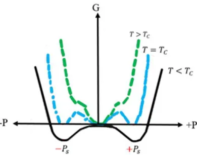
The phase transition can be understood when remembering that the stable state is the state with the lowest Gibbs free energy and looking at the Gibbs free energy versus polarization curves for temperatures above TC, equal to TC and below TC, where the two

polarization states +Ps and –Ps take place, as shown in Figure 2.6 for a ferroelectric materials with first order phase transition [26]_.

Another important characteristics of ferroelectrics is the existence of domains. In ferroelectric materials, there are microscopic domains, and within each of these domains, lined up electric dipoles are uniformly oriented along one of the crystalline directions permitted for the polarization. The application of an external electric field will orient the polarization of all domains in the direction closest to the applied field and polarize the bulk material as a whole. In general, applying a quite high electric field (of the order of hundreds of kV/cm) is necessary in order to reach the polarization saturation, i.e. the situation where all domains have the same orientation of the polarization. When removing the external electric field, most domains tend to keep their polarization oriented in the same direction, producing an effect of memory. The interface region that separates two adjacent domains is called domain wall. the domain wall motion and the energy losses related to this motion also contribute to the hysteretic behavior and to the shape of the hysteresis loop. [27]_.

Figure 2.6. Schematic potential well (Gibbs free energy G vs. Polarization P) of a ferroelectric system with first order phase transition for T>Tc, T=Tc, and T<Tc.

2.5 Magnetic Materials

Magnetism is a well-known phenomenon in nature which has attracted the attention of people since immemorial time. Magnetism is a quantum- mechanical phenomenon which occupies a central position in material science. The entities which produce magnetization and magnetize the material are known as spins. Spin is an additional degree of freedom in electronic, atomic and molecular systems. Magnetism mainly results from electrons of the atoms and molecules. Materials can be magnetically categorized into different classes: diamagnetic, paramagnetic, ferromagnetic, antiferromagnetic, and ferrimagnetic, as illustrated in Figure 2.7 [28]_.

In fact, differences in magnetic properties stem from the competition between the effect of thermal agitation and the exchange interaction. Exchange interaction is a quantum-mechanical effect occurring between identical particles. The exchange interaction depends strongly on the spin states Si and Sj of two interacting electrons according to

Heisenberg’s Hamiltonian [29] _:

𝐻 = − ∑ 𝐽_𝑖𝑗

𝑖<𝑗

𝑺_𝑖. 𝑺_𝑗

where 𝐽𝑖𝑗 is the magnetic exchange integral between 𝑆𝑖 and 𝑆𝑗.

When 𝐽_𝑖𝑗 is positive, the interaction is ferromagnetic, while when it is negative the interaction is antiferromagnetic.

2.5.1 Diamagnetic and paramagnetic materials

I. Diamagnetic materials have a zero net magnetic moment in the absence of

magnetic field. This property arises in because the electrons in their atomic orbitals are paired with spins in opposite directions. When a diamagnetic material is placed in a uniform magnetic field, it acquires a weak magnetism in the opposite direction to that of the applied magnetic field. While removing the magnetic field, magnetization disappears. It is characterized by its negative magnetic susceptibility of order 10−5 _{which is temperature independent.}

II. Paramagnetic materials possess unpaired spins oriented randomly. When the

material is subjected to an external magnetic field, the magnetic moments line up in the same direction as the field. They present a small positive susceptibility. As soon as the magnetic field is removed, the individual unpaired spins moments assume again a random orientation and the net material’s magnetic moment vanishes. Thermal agitation causes a randomization in the arrangement of the individual magnetic dipole moments so that, when the temperature increases, paramagnetic properties weaken [30]_.