A
3D
INSULIN SENSITIVITY PREDICTION MODEL ENABLES MORE PATIENT-
SPECIFIC PREDICTION AND MODEL-
BASED GLYCAEMIC CONTROLAuthors:
- Vincent Uyttendaelea,b [email protected] (corresponding author)
- Jennifer L. Dicksona [email protected]
- Kent W. Stewarta [email protected]
- Thomas Desaiveb [email protected]
- Balazs Benyoc [email protected]
- Noemi Szabo-Nemedid [email protected]
- Attila IIlyesd [email protected]
- Geoffrey M. Shawe [email protected]
- J. Geoffrey Chasea [email protected]
aDepartment of Mechanical Engineering, University of Canterbury, Private Bag 4800, Christchurch,
New Zealand.
bGIGA – In silico Medicine, University of Liège, Allée du 6 Août 19, Bât. B5a, 4000 Liège, Belgium. cBudapest University of Technology and Economics, Department of Control Engineering and
Information Technology, Budapest, Hungary
dKalman Pandy County Hospital, Dept of Intensive Care, Gyula, Hungary
eChristchurch Hospital, Dept of Intensive Care, Christchurch, New Zealand and University of Otago,
0.0 Abstract:
Background: Insulin therapy for glycaemic control (GC) in critically ill patients may improve outcomes by reducing hyperglycaemia and glycaemic variability, which are both associated with increased morbidity and mortality. However, initial positive results have proven difficult to repeat or achieve safely. STAR (Stochastic TARgeted) is a model-based glycaemic control protocol using a risk-based dosing approach. STAR uses a 2D stochastic model to predict distributions of likely future changes in model-based insulin sensitivity (SI) model-based on its current value, and determines the optimal intervention.
Objectives: This study investigates the impact of a new 3D stochastic model on the ability to predict more accurate future SI distributions, which would allow more aggressive insulin dosing and improved glycaemic control.
Methods: The new 3D stochastic model is built using both current SI and its prior variation to predict future SI distribution from 68629 hours of clinical data (819 GC episodes). The 5th-95th percentile range
of predicted SI distribution are calculated and compared with the 2D model.
Results: Results show the 2D model is over-conservative compared to the 3D case for more than 77% of the data, predominantly where SI is stable (|%ΔSI| ≤ 25%). These formerly conservative prediction
ranges are now ~30% narrower with the 3D model, which safely enables more aggressive insulin dosing for these patient hours. In addition, distributions of predicted SI within the 5th – 95th percentile range are
much closer to the ideal value of 90% for more patients with the 3D model.
Conclusions: The new 3D model better characterises patient specific metabolic variability and patient specific response to insulin, allowing more optimal insulin dosing to increase performance and safety.
Keywords: Critical Care, Insulin Sensitivity, Glycaemic Control, Blood Glucose, Hyperglycaemia, Insulin.
1.0 Introduction:
Critically ill patients in intensive care units (ICUs) often experience abnormally elevated blood glucose (BG) concentrations (hyperglycaemia), as a stress response to illness and injury [1-3]. Hyperglycaemia, glycaemic variability, and hypoglycaemia are all independently associated with increased morbidity and mortality [3-10]. Glycaemic control (GC) using insulin therapy has shown beneficial outcomes, reducing organ failure and costs [11-18]. However, other studies failed to reproduce these results [19-24], and all but two studies [25] had increased risk of hypoglycaemia with tight control. GC has been hard to achieve both safely and effectively (e.g. [26]). Fixed or ad hoc protocols are still typically used in hospitals, but fail to capture and fully account for patient variability impacting performance and safety [27]. This issue has led to the emergence of more complex, model-based GC protocols [28-30].
STAR (Stochastic Targeted) is a clinically-validated model-based GC framework, capable of adapting treatment to patient-specific insulin requirements while managing the risk of hypo glycaemia [25, 31-33]. STAR uses a patient-specific time-varying model-based insulin sensitivity (SI) to estimate patient metabolic condition. Likely future changes in SI are assessed using population-based stochastic models [34]. The 5th-95th percentile interval of BG outcomes is calculated from the 5th-95th percentile interval in
SI outcomes, allowing forward prediction of likely BG outcomes for any given insulin-nutrition
intervention. STAR thus selects an insulin-nutrition treatment to best overlap the clinically specified target BG range, while also managing and mitigating hypoglycaemic risk [32, 35], a unique risk-based dosing approach.
The stochastic model currently used by STAR forecasts future SI (SIn+1) distributions based on the identified current SI value (SIn). A Markov process is used, where outcome SIn+1 only depends on input
SIn [34]. This study expands this existing 2D stochastic approach by adding the most recent change in
SIn as an input parameter for forward prediction of outcome SIn+1. The new 3D model will now predict future SIn+1 based on current SIn and the percentage change in SI from SIn-1 to SIn. The old 2D model and the new 3D model are compared to assess the new model’s ability to tighten SI prediction ranges for tighter forward prediction of future BG. Better forward prediction of SI allows better characterisation of future metabolic variability, thus improving patient-specific glycaemic control without compromising
safety. Narrower future SI prediction ranges enable more targeted insulin dosing for these patients who are more stable. This study also assesses whether more stable patients have less future metabolic variability.
2.0 Material and Methods:
2.1 Glucose-insulin model and insulin sensitivity
The ICING (Intensive Control Insulin-Nutrition-Glucose) physiological model describing glucose-insulin dynamics is defined [25, 36, 37]: 𝐺̇ = −𝑝𝐺. 𝐺(𝑡) − 𝑆𝐼. 𝐺(𝑡) 𝑄(𝑡) 1 + 𝛼𝐺. 𝑄(𝑡) +𝑃(𝑡) + 𝐸𝐺𝑃 − 𝐶𝑁𝑆 𝑉𝐺 (1) 𝐼̇ = 𝑛𝐾. 𝐼(𝑡) − 𝑛𝐿 𝐼(𝑡) 1 + 𝛼𝐼. 𝐼(𝑡) − 𝑛𝐼(𝐼(𝑡) − 𝑄(𝑡)) + 𝑢𝑒𝑥(𝑡) 𝑉𝐼 + (1 − 𝑥𝐿) 𝑢𝑒𝑛(𝐺) 𝑉𝐼 (2) 𝑄̇ = 𝑛𝐼(𝐼(𝑡) − 𝑄(𝑡)) − 𝑛𝐶 𝑄(𝑡) 1 + 𝛼𝐺𝑄(𝑡) (3)
Where G(t) is the blood glucose level (mmol/L), I(t) is the plasma insulin concentration (mU/L), Q(t) is the interstitial insulin concentration (mU/L), P(t) is the glucose appearance in plasma from enteral and parenteral dextrose intake (mmol/min), and SI is insulin sensitivity (L/mU/min). Other parameters, rates and constants are given in [25, 36, 37] and can be found in the Additional File 1.
Model-based insulin sensitivity (SI) is patient-specific and time varying, characterising patient-specific glycaemic system response to glucose and insulin administration. SI is identified hourly from clinical BG, and insulin and nutrition input data, using an integral-based fitting method [38, 39]. This approach is robustly identifiable [40].
STAR currently uses a cohort-based 2D stochastic model to forecast future SI. As shown in Figure 1, for any current SI (SIn), the probability of SI (SIn+1) at 1-3 hours in future is determined based on a clinical data model using kernel density methods [34]. Future SI distributions used in conjunction with Equations 1 – 3 can be used to derive likely future BG distributions for a specific insulin and nutrition intervention. The 5th percentile BG prediction is used to ensure safety, limiting the maximum risk of BG
Figure 1 - Future insulin sensitivity (SIn+1) is forecasted from current insulin sensitivity (SIn). The distribution of future SI is used to predict likely BG outcomes for a given insulin-nutrition treatment intervention.
2.2 Patients and cohorts
This study uses data from 3 clinical ICU data cohorts totalling 819 GC episodes (606 patients) and 68629 hours of treatment [13, 25]:
1. Patients treated using STAR in Christchurch Hospital ICU, New Zealand, from June 2011 to May 2015.
2. Patients treated using SPRINT in Christchurch Hospital ICU, New Zealand, from July 2005 to May 2007
3. Patients treated using STAR in Kalman Pandy Hospital ICU, Hungary, from December 2011 to May 2015.
Demographics are summarised in Table 1.
Table 1 – Summary of patient demographics for the three cohorts. Results are given as median [IQR] where relevant.
SPRINT Christchurch
STAR
Christchurch STAR Gyula
# episodes 442 330 47 # patients 292 267 47 # hours 39838 22523 6268 % male 62.7 65.5 61.7 Age (years) 63 [48, 73] 65 [55, 72] 66 [58, 71] APACHE II 19.0 [15.0:24.5] 21.0 [16.0:25.0] 32.0 [28.0:36.0] LOS - ICU (days) 6.2 [2.7,13.0] 5.7 [2.5,13.4] 14.0 [8.0,20.5]
2.3 Analysis
SI level is fit on an hour-to-hour basis for each patient [38], and the forward SI variability (%ΔSI) is
defined as the hour-to-hour percentage change in SI:
%∆𝑆𝐼𝑛= 100 ×
𝑆𝐼𝑛− 𝑆𝐼𝑛−1
𝑆𝐼𝑛−1
The existing 2D stochastic model uses the input SIn to determine the outcome distribution of SIn+1. This
study builds a new 3D model to determine the outcome distribution of SIn+1 based on input of
patient-specific current metabolic state, SIn, and SI variability to current time, %ΔSIn.
A total of 66991 data triplets (%ΔSIn, SIn, SIn+1) are created from the original 68629 hours of treatment, where the number of triplets is lower because no triplets are created for the first and last hour of data. The data triplets were binned with bin sizes of %ΔSI = 10% and SIn = 0.5e-4. These bins are limited to a range of %ΔSI = [-100%, 200%] and the 1st-99th percentile range in identified SI ([1.0e-7, 2.1e-3]
L/mU/min) values, bringing the total number of triplets considered to 65051, as those few outside these ranges are excluded, corresponding to 97.1% of the original 66991 triplets.
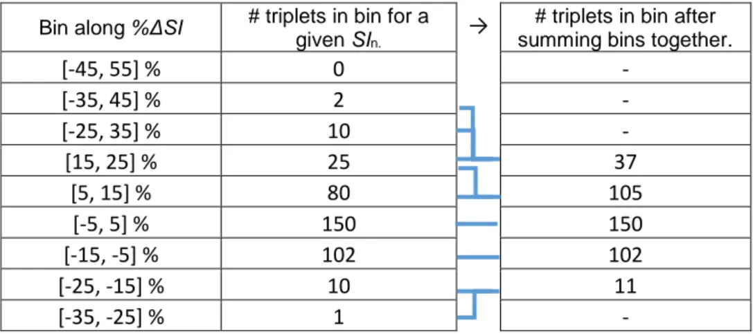
The minimum number of data points required for adequate data density in each bin was arbitrarily defined to be 100 data triplets to ensure any distributions were not influenced by outliers. To improve data density and smooth model extremes, bins not meeting this criterion are summed together along the %ΔSI axis at the same SIn level, allowing data triplets to influence neighbouring bins where there is insufficient data density. The summation process is described below, and an example is shown in Table 2.
Starting from the bin centred at 0% and going down, and at the bin centred at 10% and going up: 1. Check data density.
b. If the number of triplets < 100 add the triplets from the ‘outer’ adjacent bin(s) until data density is reached. If summation of bins still results in a failure to reach the data density, stop here.
2. Repeat step 1 until the model limits are reached.
Table 2 – Example of data density before and after the merging bin process, where the joined lines show the bins that are merged to create the final surface.
Bin along %ΔSI # triplets in bin for a
given SIn.
→
# triplets in bin after summing bins together.
[-45, 55] %
0
-
[-35, 45] %
2
-
[-25, 35] %
10
-
[15, 25] %
25
37
[5, 15] %
80
105
[-5, 5] %
150
150
[-15, -5] %
102
102
[-25, -15] %
10
11
[-35, -25] %
1
-
The 5th, 50th, and 95th percentiles of SIn+1 are computed for each bin. These values define a
non-parametric 5th – 95th percentile distribution range and median likely outcome of future variation of SI
values based on a specific current SIn level and the previous change %ΔSIn. They are interpolated linearly between bins to give a percentile surface.
To compare this new 3D model to the previous 2D model, the percentage change in the 5th, 50th, and
95th percentiles are analysed, as well as the percentage change in the 5th – 95th percentile prediction
range width used in STAR GC to select insulin dose in Figure 1. This width effectively determines the outcome BG range for a given intervention. Hence, a narrower width allows better prediction performance.
This analysis will identify regions of the model that are either conservative or have higher risk of hyper- and hypo- glycaemia. A narrowing of the 5th – 95th percentile range in the 3D model compared to the
are tighter. In contrast, wider 5th – 95th percentile range than in the 2D stochastic model indicates
increased risks, when using the 2D model, and insulin is more conservatively dosed based on this new information.
2.4 Validation
A preliminary validation of the model is carried out by assessing its ability to predict SI in clinical data episodes longer than 24 hours. The two models are compared by evaluating the per-patient percentage of SI outcomes falling into the model-predicted 5th – 95th the 25th – 75th percentile ranges for each model.
Ideally, all episodes have exactly 90% and 50% within these ranges indicating a cohort derived model that is also perfect for each patient episode. Overall, this metric gives a measure of the model’s ability to capture clinically observed patient-specific changes in insulin sensitivity [41], as well as quantifying the cohort-derived model’s level of patient-specificity. The overall goal of this comparison is a more patient-specific stochastic model.
To validate model consistency in a cohort different from which it was developed, cross simulations were used. A 3D model was built from SI traces from a randomly selected group of episodes comprising of 70% of all episodes, and tested on the remaining 30%. Per-patient percent time in the 25th – 50th and
5th – 95th percentile ranges are computed, as well as the ratio between the widths of the 5th – 95th
percentile prediction ranges for both models. This process is repeated 50 times using episodes with at least 24 hours of clinical glycaemic control data. Significant variability in results indicates a model based on too little data and/or dominated by selected patients or episodes. Consistent results indicate the model is built of enough data and/or is not skewed by outlying data. This analysis thus assesses model robustness to its underlying data.
3.0 Results:
3.1 3D model for forward prediction of SI:
The number of data triplets (%ΔSIn, SIn, SIn+1) per bin is shown in Figure 2, before and after bin merging to improve data density. The triangular shape of binned data suggests greater variability at lower SI where changes constitute a larger percentage change relative to absolute SI value. Yellow areas represent bins with enough data density (at least 100 data triplets) and thus the bins which will be used to build the model. These bins represent 62316 (95.8%) of the original 65051 triplets.
Figure 2 – Number of data triplets (%ΔSIn, SIn, SIn+1) per bin, before (a) and after (b) merging side bins (along y-axis). Bins in
yellow reach minimum data density and will be used to build the 3D model.
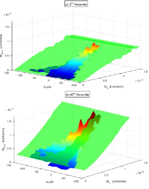
The new interpolated 3D model is shown in Figure 3 and compared to the original stochastic model (green) for the 5th (a) and 95th (b) percentiles. The previous 2D model forms a plane in the new 3D
0 0.5 1 1.5 2 x 10⁻³ -200 -100 0 100 200 300 SI n (L/mU/min) a) % SI 0 0.5 1 1.5 2 x 10⁻³ -200 -100 0 100 200 300 SI n (L/mU/min) b) % SI 0 10 20 30 40 50 60 70 80 90 100 110+
model space as it is constant across all %ΔSI. Where the new 3D model sits above the 95th percentile
or below the 5th percentile planes indicates where the 2D model was too narrow. The reverse case of
above the 5th and/or below the 95th percentile indicates the 2D model was over conservative and the
3D model 5th – 95th percentile prediction range is narrower.
The percentage change in the 5th, 50th and 95th percentiles prediction of SIn+1 is shown in Figure 4. Two
main regions can be identified:
1. A conservative region, mainly between %ΔSIn = ± 25%. The 5th percentile is higher than the
previous 2D model, while the 95th is lower, regardless of SIn, describing thus a narrower 5th –
95th percentile range in the forward prediction of SIn+1. This region represents 77.2% of the data
triplets.
2. A non-conservative region outside %ΔSIn = ± 25%. The 5th percentile is lower and the 95th is
higher, indicating higher resulting risks of hyper- and hypo- glycaemia than predicted by the 2D model. 0 0.5 1 1.5 x 10⁻³ -100 -50 0 50 100 150 SIn (L/mU/min) a) % SI 0 0.5 1 1.5 x 10⁻³ -100 -50 0 50 100 150 SIn (L/mU/min) b) % SI 0 0.5 1 1.5 x 10⁻³ -100 -50 0 50 100 150 SIn (L/mU/min) c) % SI -40 -20 0 20 40 60 80 100+ 5th Percentile 50th Percentile 95th Percentile
Figure 4 – Percentage change in the 5th (a), 50th (b), and 95th (c) percentiles between the original 2D stochastic model and the new 3D model.
Summarising Figure 4, the percentage change in the 5th – 95th percentile prediction range is shown in
Figure 5. In the 2D model’s conservative region, a significant decrease of ~25-40% in this range is observed for the 3D model, suggesting the new model allows more aggressive insulin treatment than the previous model and thus provides improved information for dose selection. For the non-conservative region, increases in SI of up to 80% or more are observed, allowing the model to more safely predict and cope with large changes in SI in regions of high metabolic variability (high %ΔSI). The reduced width green region contains 51871 data triplets (79.7%) of the total.
Figure 5 – Percentage change in the width of the 5th-95th percentile range when the new 3D model is compared to the previous 2D model. Green and red areas suggest overly conservative and under conservative behaviour respectively within the 2D model.
3.2 Self Validation
The predictive power of the new model is tested on 587 episodes of minimum 24 hours, representing a total of 63508 triplets. In total, 2.7% of these data triplets were in the initial exclusion definition and thus 97.3% of SIn+1 predictions fell within the model. Of these included values, 90.4% of SIn+1 predictions were within the 5th – 95th percentile prediction range, and 52.6% fell within the 25th – 75th percentile
range, which is very close to the expected values of 90% and 50%, respectively. The 5th – 95th percentile
interval is more critical due to its use in dosing (Figure 1). The larger error in the 25th - 75th percentile
interval versus the 5th – 95th percentile interval indicates a small mismatch in the distribution shapes
across SIn. 0 0.5 1 1.5 x 10⁻³ -100 -50 0 50 100 150 SIn (L/mU/min) % SI -40 -20 0 20 40 60 80 100 % % % % % % % %
Figure 6 presents a histogram of per-patient percentage forward prediction in the 25th-75th and 5th-95th
percentile bands, showing the accuracy at a per-patient level, rather than an overall cohort level. Table 3 shows the corresponding per-patient median [IQR] percentage time in these bands. The per-patient median [IQR] percentage time in the 25th – 75th percentile prediction range is higher in the previous 2D
model (60.3% [47.8%, 71.5%] vs. 51.2% [42.9%, 59.2%]), while the percentage time in the 5th – 95th
percentile prediction range is similar (93.6% [85.7%, 97.3%] vs. 90.7% [84.4%, 94.6%]) between the 2D and 3D models. However, as seen in Figure 6, the per-patient distributions are tighter to the ideal values (50% and 90%) for the 3D model, reducing over-conservatism.
More importantly, there was a significant reduction in the width of the 5th-95th percentile ranges for each
patient, with the 3D model reducing this width by median 28.9% [21.6%, 33.0%] per bin. These results suggest the new 3D model is able to account for changes in SI equally well in comparison to the 2D model, but with significantly narrowed prediction range for many hours of care. This outcome should allow safe application of more aggressive insulin treatments for more stable patients. An example comparison of the predictive power of the two models is shown in Figure 7.
Table 3 – Per-patient predictive power comparison between old and new stochastic model. Results are given as median [IQR].
2D Model 3D model Median per-patient % prediction within 25th-75th percentile range 60.3% [47.8%, 71.5%] 51.2% [42.9%, 59.2%] Median per-patient % prediction within 5th-95th percentile range 93.6% [85.7%, 97.3%] 90.7% [84.4%, 94.6%] Median per-patient % reduction
in 5th-95th percentile range
width
Figure 6 – Per-patient predictive power within the 25th-75th percentile prediction range (left) and within the 5th-95th percentile prediction range (right) of new (blue) and old (red) models.
Figure 7 – Excerpt from a patient showing fitted SI (blue) as well as 5th and 95th percentile prediction for the new 3D model (green) and the old 2D model (red). The new model predictive range is generally narrower than the old model.
0 0.2 0.4 0.6 0.8 1 1.2 0 10 20 30 40 50 60 70 80 90 100 Per-patient % SI n+1 within 50 th - 75th predictions # P a ti e n ts 0 0.2 0.4 0.6 0.8 1 1.2 0 20 40 60 80 100 120 140 160 180 200 Per-patient % SI n+1 within 5 th - 95th predictions 3D Model 2D Model 3D Model 2D Model 30 40 50 60 70 80 90 100 110 1 2 3 4 5 6 7 8 9 10 11 x 10-4 time (h) S I le ve l (L /m U /m in ) SI profile 90% CI - 3D model 90% CI - 2D model
Table 4 compares prediction outcomes for patients who had increased and decreased time in prediction ranges, respectively. A total of 101 episodes increased percentage time in the 5th – 95th percentile
prediction range by ~5% (87.3% [80.0%, 92.7%] vs. 82.3% [71.8%, 88.9%] for the 2D and 3D models respectively). Conversely, for the remaining 486 episodes, the new model shows slightly lower performance (91.1% [85.7%, 95.0%] vs. 94.6% [88.9%, 97.6%]). However, the percentage time in range for these patients has been brought closer to the intended 90%, ensuring the 3D model treats patients more consistently across the cohort.
Table 4 – Per-patient predictive power comparison between old and new stochastic model for two groups: 101 patients whose % prediction increased with the new model and 486 patients whose % prediction decreased. Results are given as median [IQR].
2D Model 3D model
Median % prediction within 5th
-95th percentile range for 101
patients who increased time in range.
82.3% [71.8%, 88.9%] 87.3% [80.0%, 92.7%]
Median % prediction within 5th
-95th percentile range for 486
patients who decreased time in range.
94.6% [88.9%, 97.6%] 91.13% [85.7%, 95.0%]]
3.3 Cross validation:
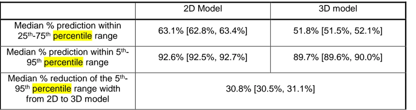
Cross-validation was carried out using patient episodes 24 hours or longer, and results are shown in Table 5. Compared to the original 2D stochastic model, the new 3D model has consistent, 12% absolute lower median [IQR] percentage forward prediction in the 25th-75th and 5th-95th percentiles ranges (3D:
51.8% [51.5%, 52.1%] vs. 2D: 63.1% [62.8%, 63.4%] and 89.8% [89.6%, 90.0%] vs. 92.5% [92.4%, 92.6%]). Additionally, the 5th-95th percentile range width from 2D to 3D model is reduced by median
30.8% [30.5%, 31.1%]. These results suggest both models generalise well to other ICU patients when developed from an independent, but similar cohort of patients, matching similar tests across cohorts [25].
Table 5 – Cross-validation per-patient results for old 2D stochastic model and the new 3D model, on all SI values from episodes of minimum 24 hours. Results are given as median [IQR].
2D Model 3D model
Median % prediction within
25th-75th percentile range 63.1% [62.8%, 63.4%] 51.8% [51.5%, 52.1%]
Median % prediction within 5th
-95th percentile range 92.6% [92.5%, 92.7%] 89.7% [89.6%, 90.0%]
Median % reduction of the 5th
-95th percentile range width
from 2D to 3D model
4.0 Discussion:
4.1 Discussion of main results
Forecasting changes in insulin sensitivity underpins the ability of STAR to respond in a patient-specific manner to potential future changes in patient glycaemic control requirements, resulting in safe and effective control strategies. If the distributions of forecast likely SI changes are narrower, then control can be further improved, with tighter control in more stable patients, and better avoidance of hypo-glycaemia in patients that exhibit high glycaemic variability. In this study, current probabilistic forecasting methods have been extended to include the change in SI (%ΔSI) as an input predictor for future SI alongside current SI.
The previous 2D stochastic model is shown to be conservative for ~77% of the data, where the %ΔSIn is within ± 25% change. While conservatism results in wider prediction ranges in likely BG outcomes, thus reducing the risk of hypoglycaemia, it also inhibits the controllers’ ability to reduce BG to the normal range using more aggressive control dosing. This issue particularly affects patients who tend to remain stable, but are mildly hyperglycaemic as a result. Hence, such conservatism, while safe, has a potentially negative clinical impact, as well.
Compared to the 2D stochastic model, a region that is over-conservative equally implies a region that is under-conservative. This under-conservative region means there are less stable patients, outside |%ΔSI| ≤ 25%, who have increased hypoglycaemic risk from relatively over-aggressive dosing, resulting from prediction bands that are too narrow. This trade off of conservatism is seen in Figures 4 and Figure 5, and offers unintended increased risk for these patients in using the 2D model.
The new model utilises change, %ΔSI, as an additional model input to better predict a more patient-specific future SIn+1, with narrowed prediction ranges for 77% of hours, and overall similar ability to meet the expected 90% of SI outcomes within the 5th-95th percentile prediction range. The new model is thus
more patient-specific, and better predicts likely BG outcomes. These results should translate into more aggressive insulin dosing where patients are more stable and SI outcomes are more certain, and less
aggressive, lower insulin doses in patients who are more variable. Greater patient-specificity also reduces risk for more variable patients. This model could thus lead to tighter and less variable control with greater safety from hypoglycaemia, and thus improved outcomes [18, 42].
Both the self-validation and the cross-validation tests have shown the predictive power of this new model to be more consistent, with closer to 90% of forward prediction of SI within the 5th-95th percentile
range. These results align well with the expected 90% of SI outcomes falling within this prediction range. However, in comparison to the previous 2D model, the new 3D model achieves this performance with overall narrower and tighter prediction distributions for 77% of hours. A median reduction in the 5th-95th
percentile prediction range width of approximately 30% was achieved with the 3D model, indicating the 3D model is better able to predict future SI outcomes, and thus safely allowing significantly increased insulin dosing.
The new 3D model thus treats patients more consistently across the patient cohort. Previously, with the 2D model, some patients within the cohort had much more than 90% of their SI outcomes within the 5th
– 95th percentile prediction range, and others much less (Figure 6). While greater conservatism is
advantageous for avoiding extreme BG outcomes, it also implies an over conservatism and inability of the model to meet its design specifications (90% of SI within the 5th -95th percentile range). Equally, it
prevents aggressive dosing and better control where it could be warranted for specific patients, and is thus less patient-specific than the new 3D model. Given the improved 5th - 95th percentile range
performance of the new 3D model, it is clear it is better able to consider patients more consistently across the cohort with the added %ΔSI model input.
Cross simulation tested the ability of the model to predict SI in patients that were not used to build the model. Cross validation results were very consistent and close to expected values from the whole-cohort analysis, suggesting that the model would generalise well to ICU patients from different protocols and/or units. It also indicates the model is not dominated by smaller outlying subsets of patients.
This result also reflects previous results where similar and consistent SI variability was seen across 3 different ICU cohorts in 3 different countries [25, 43]. This previous analysis uses slightly different patient cohorts from those presented here, and includes an additional cohort not used here. Thus, these results suggest the model generalises well to other ICU patients and cohorts, when the model is built from an independent, but overall similar cohort of mixed medical ICU patients.
4.2 Limitations
One limitation of this analysis is the binning process, which creates a discretized 3D space, where percentile surfaces were linearly interpolated between bins. Kernel-density methods, used to build the previous 2D stochastic model [34], could also be applied to generate smoother prediction percentile surfaces with respect to data density. However, this approach introduces assumptions around the shape of data density distributions and the effect of surrounding data on percentile surfaces. In this analysis, bin sizes were chosen to balance increased resolution against sufficient data density, as well as to first prove the concept.
The bin width of 10% in %ΔSI was chosen based on a previous analysis, which assessed the impact of BG measurement error on SI [44]. Given over 68,000 hours of patient data are used to build the new 3D model, the percentile surfaces of the full model are likely to be sufficiently reflective of SI dynamics, as data density was typically sufficient across typical areas of interest. Thus, limitations due to data size and density are likely to be minimal.
A further possible limitation of the model is that ~7% of data points fell outside the model range, having been discarded as outliers in regions of insufficient data density. These unusually large changes in SI or extremely high SI levels are thus not included in the model, and may reflect inaccuracies in data recording or patient-specific deviations from model-dynamics. It is also possible these points highlight times of extreme glycaemic change or measurement error, where the best clinical practice could be to discontinue insulin for an hour and come back and re-measure. In essence for these, outlying, potentially unexplained events, discontinuing insulin for a short period is a safe course of action. Within the STAR framework, the clinical usage would be to utilise the original proven 2D model, using the
safest and most conservative intervention [31, 43, 45]. Hence, points that fall in this range could be used to warn of outlying events that might not otherwise be noted, and be used to take no or more conservative action.
Overall, the new 3D model shows similar predictive performance and much tighter predictive bound when compared to the previous model. Cross-validation shows the new predictive model, constructed from bin sizes likely reflective of SI dynamics, to accurately predict SI for data not used to develop the model. These improvements in prediction should translate to tighter glycaemic control, without compromising safety from hypoglycaemia. Future work will investigate kernel-density methods to generate smoothed model surfaces, as well as exploring the management of outliers and their clinical significance.
5.0 Conclusions
Insulin sensitivity plays a major role in any model-based glycaemic control protocol and insulin sensitivity forecasting is particularly important for managing dynamic ICU patients. It thus plays a leading role in the model-based STAR protocol. In particular, it enables a patient-specific approach to achieve better control and the use of forward stochastic prediction models enables safety and performance to be explicitly balanced in determining optimal insulin dosing.
This study has shown the positive impact of identifying prior change in a proven model-based insulin sensitivity metric on the prediction of likely future insulin sensitivity distribution ranges. A new 3D model was developed, achieving similar predictive power as the previous model, while significantly reducing the width of the 5th-95th percentile prediction range for more than 77% of the hours of data. This outcome
ensures that over three-quarters of patient hours will be treated less over-conservatively. Equally, it also ensures that the remaining quarter of patient hours are not treated aggressively (under-conservatively), and thus improves safety. Both outcomes will improve the performance, safety and patient specificity of glycaemic control, and thus patient outcomes.
6.0 Abbreviations
%ΔSI Hour-to-hour percentage change in SI
APACHE Acute Physiology and Chronic Health Evaluation
BG Blood Glucose
GC Glycaemic Control
ICING Intensive Control Insulin-Nutrition-Glucose
ICU Intensive Care Unit
LOS Length of stay
SI Insulin Sensitivity
SPRINT Specialised Relative Insulin Nutrition Tables
STAR STochastic-TARgeted
7.0 Acknowledgements
The authors declare no competing interests.
VU drafted the manuscript and carried out the main analysis and results. JLD, KS, TD, and JGC expertise input in the field was necessary for results interpretation and discussion. Clinical data and clinical interpretation of the results were provided by GMS, BB, NSN, and AI. All authors had input into the redaction process.
8.0 Funding sources
The authors acknowledge the support of the EUFP7 and RSNZ Marie Curie IRSES program, the MedTech CoRE and TEC, the NZ National Science Challenge 7, Science for Technology and Innovation, the European Erasmus+ Student Mobility program, and the FRIA – Fund for Research Training in Industry and Agriculture grant.
9.0 References
![Table 1 – Summary of patient demographics for the three cohorts. Results are given as median [IQR] where relevant.](https://thumb-eu.123doks.com/thumbv2/123doknet/5443480.128079/6.892.181.712.911.1148/table-summary-patient-demographics-cohorts-results-median-relevant.webp)