HAL Id: hal-03182667
https://hal.archives-ouvertes.fr/hal-03182667
Submitted on 26 Mar 2021
HAL is a multi-disciplinary open access
archive for the deposit and dissemination of
sci-entific research documents, whether they are
pub-lished or not. The documents may come from
teaching and research institutions in France or
abroad, or from public or private research centers.
L’archive ouverte pluridisciplinaire HAL, est
destinée au dépôt et à la diffusion de documents
scientifiques de niveau recherche, publiés ou non,
émanant des établissements d’enseignement et de
recherche français ou étrangers, des laboratoires
publics ou privés.
Detection and Imaging of Magnetic Field in the
Low-Frequency Regime Using a Ferromagnetic Thin
Film Coated With a Thermo-Fluorescent Layer
Hugo Ragazzo, Daniel Prost, Jean-François Bobo, Stéphane Faure, Alexis
Chevalier
To cite this version:
Hugo Ragazzo, Daniel Prost, Jean-François Bobo, Stéphane Faure, Alexis Chevalier. Detection and
Imaging of Magnetic Field in the Low-Frequency Regime Using a Ferromagnetic Thin Film Coated
With a Thermo-Fluorescent Layer. IEEE Transactions on Magnetics, Institute of Electrical and
Electronics Engineers, 2021, 57 (3), �10.1109/TMAG.2020.3045137�. �hal-03182667�
ferromagnetic thin film coated with a thermo-fluorescent layer
H. Ragazzo
1, D. Prost
1, J-F. Bobo
2, S. Faure
3, A. Chevalier
41 ONERA/DEMR, Université de Toulouse, F-31055 Toulouse, France 2 CNRS/CEMES, Université de Toulouse, F-31055 Toulouse, France 3 LPCNO/INSA, Université de Toulouse, F-31055 Toulouse, France
4 CNRS/Lab-STICC, UMR 6285 Brest, France
Abstract— A novel and original method of LF magnetic field imaging is presented, that uses a magnetic thin film coated with fluorescent dye. Due to high permeability and consequent hysteresis losses, the film is heated by the field. As the fluorescence of the coated material is temperature-dependent, magnetic field mapping can be obtained in a short time and on a large surface by recording images with a S-CMOS camera. This principle had been previously presented in the microwave regime, for both electric and magnetic fields imaging; here we propose first results in the low frequency regime (kHz frequency range).
Index Terms— Magnetic field imaging, thermography, thermo-fluorescence, magnetic coil
I. INTRODUCTION
We propose a novel method for low frequency field measurement and imaging based on thermofluorescence. After having introduced the principles of this technique and the experimental set-up, we show that magnetic field cartography can be obtained almost instantaneously on a relatively large surface, by registering the fluorescent signal of a lighted magnetic thin film.
The characterization of electromagnetic fields emitted by various sources is an important issue, whether for civil or defense applications (magnetic coils, antennas, telecommunications, radar, civil and military aeronautics, medicine, etc.). Electromagnetic field measurement can be performed by a single probe for spatially localized results. For the visualization of the spatial distribution of magnetic fields, historically obtained from iron filings deposited on a sheet of paper, several known techniques are available [1 - 3]. Scanning systems using a moving probe are a frequent commercial solution [4]. Direct imaging of a static magnetic field has evolved with Faraday magneto-optical imaging [5] and, on a small scale, with Lorentz or holographic techniques in electron microscopy [6]. Near field measurement of integrated circuits and very large scale integration (VSLI) devices can be addressed using small probe scanning with spatial resolution of a few hundreds of microns or less [6,7]. This resolution is indeed well suited for EMC and EMI measurements and is thus recommended by international standard (IEC61967 and IEC62132) [8]. For dynamic field observation, the appropriate methods are based on stroboscopic imaging for real-time evolution of magnetic field through magnetization changes of a ferromagnetic sensor down to sub-ns scale (see for example the review by M.R. Freeman et al. [10]. However these techniques are rather complicated and time-consuming for routine characterization. It is more difficult to obtain a mapping of the magnetic field in a relatively short time. A competitive
Corresponding author: daniel.prost@onera.fr
method consists in imaging magnetic thermal losses induced by the magnetic field on a sensing foil, to obtain 2D maps of the magnetic field. This technique has been developed at ONERA for many years and is called “EMIRTM” for ElectroMagnetic InfraRed, [11].
Recently we have developed a new method that uses fluorescence thermography (called “EMVI”: ElectroMagnetic Visible Imaging) [12, 13]. Both methods use thin films which are heated by the EM field. EMIR directly records thermal frames to get field maps, whereas EMVI needs temperature dependent fluorophore coating on the film to provide visible imaging of the fluorescent light. Although this coating (and the light source exciting the fluorescence) is an additional constraint, and even if the sensitivity is reduced compared to EMIR method, the EMVI method takes advantage of the fact that it does not require a costly infrared camera and lenses. In addition, due to the respective visible vs. infrared wavelengths, EMVI offers improved spatial resolution.
To specially map the magnetic field, a high permeability ferromagnetic thin film is used which will be heated by the field because of hysteretic losses. This film can be made by patterning a ferromagnetic metallic film [14, 15]; another option is to use a commercial absorber composed of ferromagnetic micro pellets in a polymer matrix, such as Flex-Tokin thin films from TOKIN Corp. Company [16]. When those films are put into an alternating magnetic field, the amount of heat A dissipated during one cycle equals the area of the hysteresis loop [17] :
A = - µ M H dH (1)
With M(H) the magnetization of the ferromagnetic particles. Then for a given frequency f we have the specific absorption rate (SAR) :
Page 2 of 6
————————————————————————————————————–
SAR = A.f (2)
The fluorescent coating is a thin rhodamine-B layer embedded in epoxy resin, which presents linear temperature-dependent properties: therefore, having illuminated the film (with LED source), magnetic field-dependent fluorescence images are provided in the visible range. Then, a S-CMOS camera records the variation of fluorescence intensity. To improve the sensibility, accuracy and dynamic of the EMVI measurement, we use the lock-in thermography technique. The principle is to modulate the EM source at low frequency and evaluate only the oscillating part, at the same frequency, of the detected signal [18, 19].
We have shown in a precedent paper how this technique can give field cartographies in microwaves domain [20]. Here we show the capacity of this method to cartography magnetic field at much lower frequency (kHz). We choose a simple and known system to demonstrate this: a magnetic flat-coil. This kind of coil is used in many systems like induction cooker.
In section II we detail the experimental set up and flat coil characteristics. Section III is devoted to different characterizations of the sensitive film: we investigate the chemical composition, the shape of the ferromagnetic micro-particles, the permeability and the thickness of the film. In section IV we show the images of the magnetic field of the flat-coil that thermo-fluorescence can provide. Those are compared with numerical simulations, and the effect of an effective anisotropy observed in the thin film will be discussed and fixed. Finally, we comment about different advantages of this technique and possible development.
II. FLAT COIL AND EXPERIMENTAL SET UP
A. Flat coil characteristic
As mentioned above, the EMVI method has been demonstrated in the microwave frequency range. We choose here a kHz coil to test the wideband capacity of EMVI. Moreover, this flat-coil is simple to simulate and the distribution of the magnetic field is almost uniform below the coil. Our flat coil has the following characteristics (see Fig. 1):
• Outside diameter: 95 mm • Inside diameter: 6 mm • 20 turns with 2-mm² Litz wire • Self-inductance: L = 0.605 µH
(a) (b)
Fig. 1. a) Flat-coil; b) dimensions and film location.
The resonance frequency of the coil is driven by the LC circuit, and we have (with C ≅ 500 nF and L ≅ 700 nH :
f = √ = 271 kHz (3)
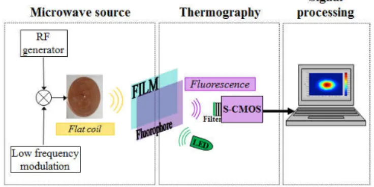
B. Experimental set up
Fig. 2 is the schematics of the EMVI set up. The coil is supplied at its resonant frequency (f0 = 271 kHz), with a low frequency square modulation at 0.2 Hz.
The thermo-fluorescent film is located 5 mm above and parallel to the flat-coil. The fluorescence is excited by a LED array delivering a 470 nm monochromatic light, with a measured power density of almost 3.2 mW.cm-2. The S-CMOS camera is located 20-cm in front of the film. We add a low-pass 580 nm filter in order to collect only the fluorescence signal ; as the emitted magnetic field heats the film, the temperature-dependent fluorescence intensity of the rhodamine-B is affected (this is the principle of the method of measurements). The lock-in thermography method is used, that is to say that the fluorescent frames recorded by the camera are demodulated (at 0.2 Hz) to eliminate continuous thermal phenomena (conduction in the film, convection) [21]. Considerations related to image processing led us to record nearly 10 periods with 20 images per second (almost 1000 images), giving a total acquisition time of less than one minute. This allows reaching a thermal resolution of less than 50 mK.
Fig. 2. EMVI setup schematics.
III. CHARACTERIZATION OF THE FILMS
A. Microstructure characterization
The commercial absorber films (TOKIN Flex Suppressor) are magnetic composites made by blending micro sized magnetic material powders in a polymer base. Their good electromagnetic absorption properties lie in their structure where ultra-thin magnetic metal foils of the micron order overlap each other in the same direction. Three thicknesses are available for the selected TOKIN’s films: 300 µm, 100 µm and 30 µm. In a first step, we have used scanning electron microscope to investigate the size, shape and orientation of the micro-particles of the films. We present results of the thicker film which exhibits the best image contrast. Fig. 3 shows scanning electron microscope images of the 300-µm TOKIN’s film.
Coil Film
5 mm
Φin 6 mm
————————————————————————————————————–
µV 800 V curr 86 pA Mag 1 000x WD 6.6 mm Det ETD HFW 207 µm (a) (b)Fig. 3. (a) Surface scanning electron microscope image and (b) Optical microscope image of 300-µm TOKIN’ film (mag. x 5).
In Fig. 3 (a), we have in dark grey the polymer and in light grey the particles. Particles are randomly dispersed micron sized flakes embedded in the polymer matrix. Easy axis of the magnetization stands therefore in the plane of the flakes. This leads to an macroscopic easy-axis of magnetization in the plane of the foil. We also observed the sample with optical microscope, exhibiting transversal lines due to the lamination process (Fig. 3 (b)). The lamination process can be a potential cause for an additional in-plane anisotropy, which leads to different behaviors in two perpendicular in-plane directions. We confirm this point by the magnetic measurement presented in section B.
For our measurements, we only used 30-µm thick TOKIN’s film. Indeed the 300 and 100-µm thick films absorb too much of the magnetic energy and would have been too much intrusive. These thicker films were indeed found to change the resonance frequency of the flat coil while the 30-µm film had no significant effect. Furthermore, the shape anisotropy of these films composed of ferromagnetic pellets may alter the spatial distribution of the magnetic field to be probed as a shield. All these reasons justify our choice of the 30-µm film.
B. Magnetic losses Characterization
As the EMVI method takes advantage of the absorbed electromagnetic power that heats the material, it is important to analyze the magnetic losses of the films. Two types of losses occur simultaneously in magnetic materials: i) the hysteresis process and ii) the dispersion process due to the domain wall
motion and spin resonance [22]. Thus, the electromagnetic power absorbed in the material will depend on both the amplitude and the frequency of the magnetic field.
Fig. 4 (a) shows the static hysteresis loops measured for two perpendicular orientations of the 30 µm TOKIN’s films. Coercivity is very low; films show very soft magnetic properties. The magnetic behavior depends on the orientation of the sample that indicates the presence of an anisotropy. Since there is no preferential grain orientation, the lamination process probably causes this anisotropy as shown in Fig. 3 (b) with the observed transversal streak of lines.
In order to take into account the frequency effects on the magnetic losses, we investigated the dynamic hysteresis loop at 270 kHz, close to the resonance frequency of the flat coil. A specific hysteresis meter based on the transformer method and lock-in amplifiers was used to measure the magnetization M of the sample under a dynamic magnetic field H [23]. The apparatus allows tuning both the frequency and the magnitude of the magnetic field. Fig. 4 (b) shows the dynamic hysteresis loops measured at 270 kHz for the maximal field’s strength allowed by the apparatus at this frequency for the two orientations of the 30-µm TOKIN’s films. Again, the behavior depends on the orientation. The magnetic susceptibility (M/H slope) is different depending on the orientation; moreover, the surfaces of the loops are different. The specific absorption rate is greater in the parallel direction than in the perpendicular one. Thus, the film will heat more in the parallel direction.
(a)
(b)
Fig. 4. (a) Static magnetization and (b) Dynamic magnetization curve of a 30-µm TOKIN’s film square sample for two orientations. 50 µm
Page 4 of 6
————————————————————————————————————–
C. Study of the thickness of the fluorescent layer The magnetic thin film is coated with a fluorescent layer whose thickness has been measured using confocal microscopy. It is important to control this thickness (the fluorescence layer) because perturbing thermal effects induced in our sample are function of this thickness, in particular thermal diffusion. A thermal wave with a frequency (ω) has a thermal diffusion length (D), which can be expressed as:
D = %'(&) (4)
Where k is the thermal conductivity (W.m-1.K-1), Cp is the specific heat capacity (J.kg-1· K-1), and ρ the density (kg.m-³). In the case of TOKIN film, D is about 100-500-µm for a modulation between 0.1 and 3 Hz.
If e < D with e the thickness of the sample (magnetic + fluorescent layers), we are in the case of a 2D film approximation and the heat equation can be simplified [13]:
ρC+,-,. = P012 t 4 65∗ T 4 T69: (5)
With T the temperature (K), Pabs the incident magnetic power absorbed by the film (W), h the heat transfer coefficient (W.m2.K-1) between the film and the environment, and T
env the temperature of the environment (K).
The fluorescent layer is composed of a fluorophore diluted in ethanol, and then embedded in epoxy resin. rhodamine-B was chosen for two reasons: its absorption spectrum is separated from its emission spectrum, and its fluorescence intensity presents a linear behavior with heating (of 1.8 %.K-1 in our temperature range [13]). An average thickness of 29 µm was measured for the fluorescent layer (using confocal measurement), standing from 20 µm to 32 µm. Therefore, the total thickness is about 59 µm. We therefore stay in the case of 2D film approximation (e < D). In other words, we consider that the temperature is homogeneous in the total (TOKIN magnetic film + fluorescent layer) thickness: when the magnetic film is heated by the field, the fluorescent layer temperature increases with a negligible delay (compared to the low frequency modulation). It follows that on the steady state, where the phase shift is neglected, the heating amplitude at the modulation frequency ω is proportional to the magnetic absorbed power and given by [13]:
T;<== >?@6
%A5BC )6ωB (6)
IV. RESULTS AND DISCUSSION
A. Images and simulation of the magnetic field of the flat-coil
We therefore visualized the magnetic field with the 30-µm thick film coated with 28 µm of RhB-epoxy fluorophore. The feeding current intensity in the flat-coil is: DEFGH = 14 J and the modulation frequency: KLFM= 0.2 OP. The film was located 5 mm away from the surface of the coil (see Fig. 1). The measured variation of fluorescence intensity, ∆Ifluo, is
normalized by the mean fluorescence intensity <Ifluo>. This
normalization avoids inaccuracies due to fluorophore thickness variations.
(a)
(b)
(c)
Fig. 5. Mapping of the magnetic field Bxy tangential component of the
flat-coil (a) EMVI Mapping, (b) EMVI Mapping averaged over four images with a film rotation of 0°, 90°, 180° and 270°, (c) Analytical calculation of the tangential component of the magnetic field.
————————————————————————————————————–
Using the Biot-Savart law, applied on numerically segmented coil, we can easily calculate the tangential component of the magnetic field of the flat-coil.As expected, Fig. 7 (c) shows that the calculated tangential component of the magnetic field is equal to zero at the center and has a radial distribution above the coil.
Instead of getting the calculated isotropic field pattern of the Fig. 5 (c), we first observe a difference in measured intensity along the x and y axis in Fig. 5 (a). This is consistent with the anisotropy observed on the magnetic measurements in section III. To fix this issue, since the film has a perpendicular magnetic anisotropy, we performed four measurements with successive rotation of 90, 180, and 270° around its center. Fig.
5 (b) shows the demodulated fluorescence intensity image averaged over those four measurements: the anisotropy has thus disappeared on Fig. 5 (c).
Fig. 6. Comparison measured and calculated magnetic field profiles on x-axis (magenta) and y-axis (green) and black dotted lines on Fig. 5 (b) and (c).
As the fluorescence depends on magnetic energy, the magnetic field is proportionally linked to the square root of the fluorescence intensity. The corresponding coefficient kH can be determined by comparing simulation and measurement. We thus have:
H = k %∆RSTUV
WRSTUVX (7)
where kH depends on the heat capacity, the modulation frequency, the thickness of the sample and the magnetic losses of the film. We obtain herekH = 6.53 10-3 A.m-1.K-1/2..
Fig. 6 shows a comparison of profiles taken along two perpendicular directions on the averaged EMVI image (Fig. 5 (b)) and analytical calculation image (Fig. 5 (c)). The film anisotropy is properly suppressed by averaging the fluorescence signal. At the center of the coil we observe a discrepancy between the measurement and the calculation. We observe a weak heating of the coil during the experimentation due to Joule effect. We assume that the coil’s heating adds a heat source by convection that is at the origin of the weak component at the center of the coil. The coil’s heating time scale is similar to the modulation frequency of the current
inside the coil and therefore adds a parasite contribution to the demodulated signal.
B. Remark on the light environment
For thermo-fluorescence measurement, it is obviously better to stay in a dark room, to avoid daylight noise perturbations. This aspect could be problematic for applications. For this reason, we performed measurements under external lighting, and compared with previous (dark room) measurement in order to evaluate the sensitivity to that external noise. The measurement was achieved in shed light from neon and natural light. We stayed in the same experimental conditions to allow comparison: the feeding current intensity in the flat-coil is also: DEFGH= 14 J and the modulation frequency: KLFM= 0.2 OP.
(a) (b)
Fig. 7. Image of magnetic field of a flat-coil (a) in dark room, (b) under light.
The measured power density of the light in front of the camera in the two environments (dark room and lit room) shows a huge difference: we have more than two orders of magnitude:
• Pdark = 0.52 µW.cm-2 • Plight = 90.5 µW.cm-2
Using two sources of green LED spots, we increased the power density of the excitation light, and therefore the amplitude of the fluorescence signal (up to a few mW.cm-2). This allowed us to decrease the exposition time of the camera and to be less sensitive to external light. By this way, the noise due to natural light can be minimized. We compared the signal-to-noise ratio (SNR), calculated from the power spectrum, of every pixel. The SNR follows a normal distribution. In the case of the SNR under external light we obtain a mean value of 12.5 dB (with standard deviation = 2.5 dB); without external light, the SNR is only slightly degraded since we have a mean value of 14 dB (with standard deviation = 3 dB).
To conclude we consider that the EMVI measurement is only slightly degraded under shed light (compared to dark room conditions), and remains operational as a magnetic field mapping measurement method.
V. CONCLUSION
Magnetic field imaging was performed for the first time in the 100 kHz range using thermo-fluorescent thermography. It makes it possible to obtain 2D cartography of the field in a few
Page 6 of 6
————————————————————————————————————–
minutes, independently of the size of the film, which can be faster than using a scanning process with a point probe. As the process is also well suited to microwave regime, this original method could have many applications.
The magnetic film and fluorescent coating were deeply investigated using several characterization techniques (microscopy, confocal measurement, magnetic characterization), showing an anisotropic magnetic behavior. However, the anisotropy issue was fixed by averaging measurements in the different directions.
Last, we showed that even if a dark room environment is preferable, thermo-fluorescent images could be obtained in a lit room without strong degradation of the results.
REFERENCES
[1] J. Lenz, A.S. Edelstein, “Magnetic sensors and their applications,” IEEE Sensors Journal, vol. 6, no. 3 , pp. 631-649, June 2006, doi: 10.1109/JSEN.2006.874493.
[2] D. Tomasi, H. Panepucci, “Magentic fields mapping with the phase reference method,” Magnetic Resonance Imaging, vol. 17, no. 1, pp. 157–160, Feb. 1999.
[3] M. Blagojevic, D. Mancic, “The system for magnetic field mapping based on the integrated 3D Hall sensor,” 24th Telecommunications Forum
(TELFOR), 2016.
[4] SENIS, “All-in-One Standard Magnetic Field Mapper MMS-1A-R”,
https://www.senis.ch/.
[5] V. Kochergin, “Magnetic Field and Electrical Current Visualization System,” US patent, no. US6,934,068B2, 2005.
[6] K. Slattery and Wei Cui, "Measuring the electric and magnetic near fields in VLSI devices," 1999 IEEE International Symposium on Electromagnetic Compatibility. Seattle, WA, USA, 1999, pp. 887-892 vol.2, doi: 10.1109/ISEMC.1999.810172.
[7] K. P. Slattery, J. W. Neal and Wei Cui, "Near-field measurements of VLSI devices," in IEEE Transactions on Electromagnetic Compatibility, vol. 41, no. 4, pp. 374-384, Nov. 1999, doi: 10.1109/15.809825. [8] International Electrotechnical Commission: IEC-61967 (Integrated
circuits - Measurement of electromagnetic emissions), IEC-62132 (Integrated circuits - Measurement of electromagnetic immunity). [9] E. Snoeck, C. Gatel, L. M. Lacroix, T. Blon, S. Lachaize, J. Carrey, M.
Respaud, B. Chaudret, “Magnetic Configurations of 30 nm Iron Nanocubes Studied by Electron Holography,” Nano Lett. 2008, vol. 8, no.12, pp. 4293–4298.
[10] M.R. Freeman, A.K. Hiebert, “Stroboscopic microscopy of magnetic dynamics,” Spin Dynamics in Confined Magnetic Structures I - Topics in Applied Physics, vol. 83, ed. B Hillebrands and K Ounadjela (Berlin: Springer) pp. 93–126, 2002.
[11] P. Levesque, L. Leylekian, “Capteur vectoriel de champs électromagnétique par thermographie infrarouge,” French Patent, no. 9816079, 1998.
[12] S. Faure, J.F. Bobo, J. Carrey, F. Issac and D. Prost, “Sensitive component for device for measureing electromagnetic field by thermofluorescence, corresponding measurement and manufacturing methods,” based on French Patent Application, no. 1758907, 2017. [13] S. Faure, J-F. Bobo, D. Prost, F. Issac, and J. Carrey, “Electromagnetic
Field Intensity Imaging by Thermofluorescence in the Visible Range,” Phys. Rev. Applied, vol. 11, p. 054084, Mar. 2019.
[14] J. Vernieres, J.F. Bobo, D. Prost, F. Issac, F. Boust, “Ferromagnetic microstructured thin films with high complex permeability for microwave applications,” J. of Appl. Phys., vol. 109, p. 07A323, Mar. 2011.
[15] J. Vernieres, J.F. Bobo, D. Prost, F. Issac, and F. Boust, “Microwave magnetic field imaging using thermo-emissive ferromagnetic microstructured films,” IEEE Trans. Magn., vol. 47, no. 9, pp. 2184-2187, Sept. 2011, doi: 10.1109/TMAG.2011.2138150.
[16] https://www.tokin.com/english/product/pdf_dl/flex.pdf.
[17] J. Carrey, B. Mehdaoui, and M. Respaud, “Simple models for dynamic hysteresis loop calculations of magnetic single-domain nanoparticles: application to magnetic hyperthermia optimization,” J. Appl. Phys., vol. 109, 083921, Apr. 2011.
[18] S. Huth, O. Breitenstein, A. Huber and U. Lambert, “Localization of gate oxide integrity defects in silicon metal-oxide-semiconductor structures with lock-in IR thermography,” J. Appl. Phys., vol. 88, 4000, Sep. 2000. [19] G. breglio, A. Irace, L. Maresca, M. Riccio, G. Romano and P. Spirito,”Infrared thermography applied to power electron devices investigation,” Facta Universitatis, Series: Electronics and energetics, vol. 28, no. 205, Jan. 2015.
[20] H. Ragazzo, S. Faure, J. Carrey, F. Issac, D. prost and J.F. Bobo,”Detection and imaging of magnetic field in the microwave regime with a combination of magnetic losses material and thermofluorescence molecules,” IEEE Trans. Magn., vol. 55, no. 2, pp. 1-4, Feb. 2019, Art no. 6500104, doi: 10.1109/TMAG.2018.2860520.
[21] D.L. Balageas, P. Levesque, and A. Déom, “Characterization of electromagnetic fields using lock-in IR thermography,” Thermosense XV, SPIE vol. 1933, pp. 274-285, Apr. 1993.
[22] J. B. Goodenough, “Summary of losses in magnetic materials,” IEEE Trans. Magn., vol. 38, no. 5, pp. 3398-3408, Sept. 2002, doi: 10.1109/TMAG.2002.802741.
[23] T. Shirane and M. Ito, “Measurement of hysteresis loop on soft magnetic materials using lock-in amplifier,” IEEE Trans. Magn., vol. 48, no. 4, pp. 1437-1440, April 2012, doi: 10.1109/TMAG.2011.2174147.