HAL Id: hal-01152443
https://hal.archives-ouvertes.fr/hal-01152443
Submitted on 20 May 2015
HAL is a multi-disciplinary open access archive for the deposit and dissemination of sci-entific research documents, whether they are pub-lished or not. The documents may come from teaching and research institutions in France or abroad, or from public or private research centers.
L’archive ouverte pluridisciplinaire HAL, est destinée au dépôt et à la diffusion de documents scientifiques de niveau recherche, publiés ou non, émanant des établissements d’enseignement et de recherche français ou étrangers, des laboratoires publics ou privés.
fiber-reinforced composite materials in the case of
debonded fibers
Yahya Berrehili, Jean-Jacques Marigo
To cite this version:
Yahya Berrehili, Jean-Jacques Marigo. The homogenized behavior of unidirectional fiber-reinforced composite materials in the case of debonded fibers. Mathematics and Mechanics of Com-plex Systems, International Research Center for Mathematics & Mechanics of ComCom-plex Systems (M&MoCS),University of L’Aquila in Italy, 2014, 2 (2), pp.181-207. �hal-01152443�
S’ESSA NON PASSA PER LE MATEMATICHE DIMOSTRAZIONI LEONARDO DA VINCI
Mathematics and Mechanics
of
Complex Systems
msp
vol. 2
no. 2
2014
YAHYABERREHILI AND JEAN-JACQUESMARIGO
THE HOMOGENIZED BEHAVIOR OF
UNIDIRECTIONAL FIBER-REINFORCED COMPOSITE MATERIALS IN THE CASE OF DEBONDED FIBERS
Vol. 2, No. 2, 2014
dx.doi.org/10.2140/memocs.2014.2.181 M\M
THE HOMOGENIZED BEHAVIOR OF
UNIDIRECTIONAL FIBER-REINFORCED COMPOSITE MATERIALS IN THE CASE OF DEBONDED FIBERS
YAHYABERREHILI AND JEAN-JACQUESMARIGO
This paper is devoted to the analysis of the homogenized behavior of unidirec-tional composite materials once the fibers are debonded from (but still in contact with) the matrix. This homogenized behavior is built by an asymptotic method in the framework of the homogenization theory. The main result is that the homog-enized behavior of the debonded composite is that of a generalized continuous medium with an enriched kinematics. Indeed, besides the usual macroscopic displacement field, the macroscopic kinematics contains two other scalar fields. The former one corresponds to the displacement of the matrix whereas the two latter ones correspond to the sliding and the rotation of the debonded fibers with respect to the matrix. Accordingly, new homogenized coefficients and new cou-pled equilibrium equations appear. This problem is addressed in a linear elastic three-dimensional setting.
1. Introduction
The use of unidirectional fiber-reinforced composite materials does not cease to grow in various domains and particularly in the domains of aerospace and aero-nautics. This is due to their various properties and especially to their interesting mechanical behavior in terms of their specific effective stiffness in the direction of the fibers. (Throughout the paper, the word effective is a synonym of homogenized or macroscopic.) The effective elastic behavior of such composites is now well known and well modeled by the homogenization theory as long as the fibers are assumed to be perfectly bonded to the matrix [Léné 1984; Michel et al. 1999; Sánchez-Palencia 1980; Suquet 1982].
However, since their mechanical performance is considered optimal when the components remain bonded, it remains to evaluate the loss of performance when
Communicated by Pierre Seppecher.
This work was partially supported by the French Agence Nationale de la Recherche (ANR), under grant epsilon (BLAN08-2_312370) “Domain decomposition and multi-scale computations of singu-larities in mechanical structures”.
MSC2000: 35C20, 35J20, 74B05, 74G10, 74Q15.
Keywords: homogenization, composite materials, debonding.
the fibers are debonded. Of course, if one considers that the elastic behavior is due to the matrix alone, the specific stiffness drops drastically. But this type of estimate simply gives a lower bound to the stiffness and one must define more precisely the effective behavior of completely or partially debonded unidirectional composites. Many works have been devoted to this task; see for instance [Bouchelaghem et al. 2007; Caporale et al. 2006; Gonzàlez and LLorca 2007; Greco 2009; Jendli et al. 2009; Kulkarni et al. 2009; Kushch et al. 2011; Léné and Leguillon 1982; Marigo et al. 1987; Matouš and Geubelle 2006; Moraleda et al. 2009; Teng 2010]. In general, these studies consist in replacing the perfect bond of the interface by some “cohesive law” or simply in removing the fibers when the debonding is complete.
In any case, the calculation of the new homogenized mechanical coefficients is per-formed by considering the usual elementary problems set on the unit cell without reconsidering the general procedure of homogenization. However, when following the two-scale asymptotic approach, it appears that the argument used to obtain that the zero-order displacement field does not depend on the microscopic variable is no longer valid. Therefore, in the zone where the fibers are debonded, the macroscopic displacement field must be replaced by another “macroscopic” displacement field, corresponding to the independent displacement of the fibers [Berrehili and Marigo 2010]. Consequently, one must also construct the macroscopic problem which gives this additional field. That is the purpose of this paper.
Specifically, the paper is organized as follows. The next section is devoted to the setting of the problem: one considers a composite structure , constituted by a periodic distribution of elastic unidirectional fibers whose direction is e3 and
embedded in an elastic matrix. In a part c of the fibers are assumed to be
bonded to the matrix whereas in the complementary part d they are assumed to be
debonded but still in contact without friction with the matrix. We then formulate the elastostatic problem which contains the small parameter ✏ related to the size of the microstructure and which governs the displacement fieldu✏ and the stress field ✏.
The third section is devoted to the asymptotic analysis, i.e., the behavior ofu✏
and ✏ when ✏ goes to 0. Following a two-scale approach, we first postulate thatu✏
and ✏ can be expanded in powers of ✏, the coefficientsui(x, y) and i(x, y) of
the expansion being periodic functions of the microscopic coordinates y. We then obtain a sequence of variational equations in terms of the ui and the i. These
equations are sequentially solved to finally obtain the effective behavior of the composite in its bonded and debonded parts. In the fourth section, we study the properties of the effective model and, in particular, the properties of the effective coefficients provided by the solutions of linear elastic problems posed either on the bonded or on the debonded cell. Then, some examples are treated. We finally conclude giving some perspectives.
The set of real numbers, the set of n-dimensional vectors and the set of symmetric second-order n-dimensional tensors are, respectively, denoted byR,Rn andMns. Vectors and second-order tensors are indicated by boldface letters, like u and for the displacement field and the stress field. Their components are denoted by italic letters, like ui and i j. Fourth-order tensors as well as their components are
indicated by sans-serif letters, likeAorAi jkl for the stiffness tensor. Such tensors
are considered as linear maps acting on second-order tensors. The application of Ato " is denotedA", with componentsAi jkl"kl. The inner product between two
vectors or two tensors of the same order is indicated by a dot, like a · b which stands for aibi or · " for i j"i j. The symbol ⌦ denotes the tensor product and
⌦s denotes its symmetric part; i.e., 2e1⌦se2= e1⌦ e2+ e2⌦ e1.
In our frequent use of multiple scaling techniques, we adopt the related nota-tion. For instance,x = (x1,x2,x3)always denotes a macroscopic coordinate while
y = (y1,y2) represents a microscopic one. Since the fibers are oriented along
the directione3, we distinguish the longitudinal coordinate x3 from the transversal
coordinatesx0= (x1,x2). Latin indices run from 1 to 3, while Greek indices run
from 1 to 2. When a spatial (scalar, vectorial or tensorial) field depends both onx and y, the partial derivative with respect to one of the coordinates appears explicitly as an index: for example,divx and "x(v)denote, respectively, the divergence of the stress tensor field and the symmetric gradient of the vector field v with respect tox, while divy and "y(v)are the corresponding derivatives with respect to y:
divx (x, y) = @ i j @xj (x, y)ei, divy (x, y) = @ i @y (x, y)ei, (1) "x(v)(x, y) = ✓ @vj @xi(x, y) + @vi @xj(x, y) ◆ ei⌦sej, (2) "y(v)(x, y) = ✓ @v↵ @y (x, y) + @v @y↵ (x, y) ◆ e↵⌦se + @v3 @y↵ (x, y)e↵⌦se3. (3)
On a surface I across which a field f is discontinuous, we denote by [[ f ]] its jump discontinuity.
2. Statement of the problem
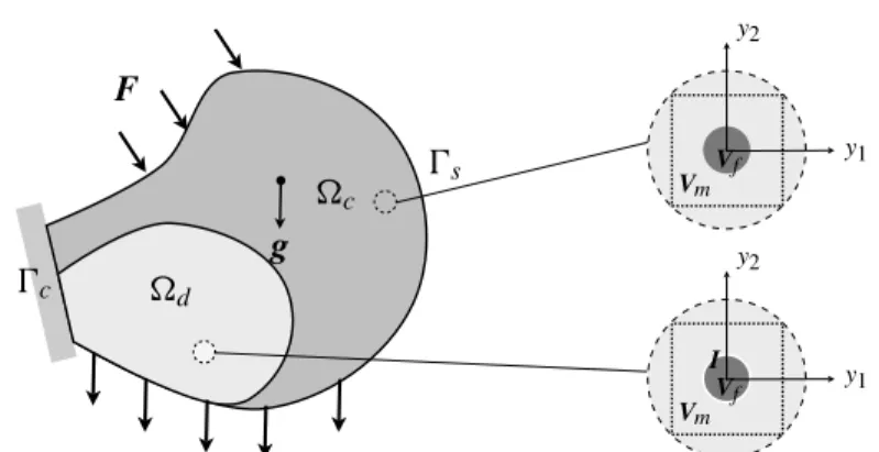
We consider a heterogeneous elastic body whose natural reference configuration is a bounded open domain ofR3with a smooth boundary @. We denote by (e1,e2,e3)the canonical basis ofR3and by (x1,x2,x3)the coordinates of a point x 2 . The body is made of two isotropic linearly elastic materials, called the fibers and the matrix, whose Lamé coefficients and mass density are, respectively, ( f, µf, ⇢f)and ( m, µm, ⇢m). The fibers are aligned in the directione3and have
F 0c d g c 0s y2 y1 Vf Vm y2 y1 I Vf Vm
Figure 1. The composite structure and the two periodic cells.
matrix, ✏a and ✏b being the two vectors of the plane (e1,e2)characterizing the periodicity. The number of fibers is large so that the dimensionless parameter ✏ characterizing the fineness of the microstructure (for instance, the ratio between the spatial period and the size of the structure) is small. The domain occupied by the fibers is ✏
f, that occupied by the matrix is ✏m, while the set of all interfaces
between fibers and matrix is I✏. Accordingly, one has
= ✏f [ I✏[ ✏m. (4)
The fibers are perfectly bonded in a part c of and debonded in the
complemen-tary part d; see Figure 1. Both parts contain a large number of fibers and will
be considered as given and independent of ✏. Moreover we assume that in d the
fibers remain in contact with the matrix but can slip without friction. Accordingly, denoting by
I✏
c = c\ I✏, Id✏ = d\ I✏, (5)
respectively, the bonded and debonded interfaces, the interface conditions in terms of the displacement and the stress fields read as
⇢ [[u]] = 0, [[ ]]n = 0 on I✏
c,
[[u]] · n = 0, [[ ]]n · n = 0, n^n = 0 on I✏ d.
(6) In (6),n is the outer normal to the fiber at an interface and the brackets denote the jump of the involved field across the interface. The conditions on I✏
c mean that
the displacement and the vector stress are continuous; the conditions on I✏
d mean
that the normal displacement and the normal stress are continuous while the shear stress vanishes.
Remark 1. In the above conditions on the interface between the fibers and the matrix after debonding, we assume that contact always occurs without friction. This allows us to treat linear elastic problems and then the analysis is simplified.
It would be easy to follow the same procedure by assuming that the fibers are no longer in contact with the matrix after debonding. It is more difficult to consider unilateral frictionless contact conditions where the contact conditions depend on the sign of the normal stress. That leads to nonlinear (but still elastic) problems where the superposition principle can no longer be used. Much more difficult is the case where the contact occurs with friction. Then the effective behavior is no longer elastic and one must introduce internal variables. All these more elaborated cases are outside the scope of this didactic paper and will be the subject of future works.
The body is submitted to a specific body force density g (independent of ✏). The part 0c of the boundary @ is fixed while the complementary part 0s= @ \ 0c is
submitted to a surface force density F (independent of ✏).
We are now in a position to set the problem which governs the response of the body at equilibrium under the given loading. For a fixed ✏ > 0, the problem consists in finding a displacement field u✏ and a stress field ✏, such that:
Equilibrium: ⇢div ✏+ ⇢fg = 0 in ✏f, div ✏+ ⇢ mg = 0 in ✏m, (7) Constitutive relations: ⇢ ✏ = f divu✏ + 2µf"(u✏) in ✏f, ✏= mdivu✏ + 2µm"(u✏) in ✏m, (8) Compatibility: 2"(u✏)= ru✏+ rTu✏ in ✏ f [ ✏m, (9) Boundary conditions: ⇢ u✏✏ = 0 on 0c, n = F on 0s, (10) Interface conditions: ⇢ [[u✏]] = 0, [[ ✏]]n = 0 on I✏ c, [[u✏ n]] = 0, ✏n = nn✏ n, [[ nn✏ ]] = 0 on Id✏. (11) In (8), is the identity tensor with i j= 1 when i = j and i j= 0 when i 6= j. This
set of equations constitutes a linear boundary value problem which can be written in a variational form as follows.
Let#✏ be the linear space of kinematically admissible displacement fields; i.e.,
#✏= v 2 H1(\ I✏
d;R3): [[v]] · n = 0 on Id✏, v= 0 on 0c , (12) letf✏ be the continuous linear form associated with the applied forces; i.e.,
f✏(v)= Z ✏f ⇢fg · v dx + Z ✏ m ⇢mg · v dx + Z 0s F · v d0 for v 2#✏, (13)
and leta✏ be the bilinear continuous form associated with the elastic energy; i.e.,
a✏(u, v) = Z ✏f Af"(u) · "(v) dx + Z ✏ m Am"(u) · "(v) dx. (14)
In (14),Af andAm stand for the fourth-order elasticity tensors of the fibers and the matrix, respectively; i.e.,
Ai jklf,m= f,m i j kl+ µf,m( ik jl+ il jk). (15)
Thenu✏ must satisfy the variational problem
findu✏ 2#✏ such thata✏(u✏, v)=f✏(v)for all v 2#✏, (16)
and ✏ is the associated stress field given in terms of the strain field by (8). The
existence and the uniqueness of the solutionu✏ of (16) is guaranteed provided that
the boundary 0c is such that there does not exist any (nonzero) rigid displacement
which is kinematically admissible. Specifically, let us denote by 5✏ the set of
displacement fields which are both kinematically admissible and corresponding to a null strain field; i.e.,
5✏= {v 2#✏: "(v) = 0 in \ I✏
d}. (17)
By standard arguments, we have:
Proposition 1. Under the condition that5✏ = {0} and that the density of forces
g and F are smooth enough, the variational problem (16) admits a unique solu-tionu✏.
The necessary and sufficient condition above for the existence and the unique-ness of the solution depends in general both on 0c and d. However, the existence
of a solution is guaranteed if5✏= {0}, that is, if no rigid displacements are allowed.
We will assume henceforth that this condition is satisfied. 3. Asymptotic analysis
This section is devoted to the behavior ofu✏, the unique solution of (16), when ✏
goes to 0. For that we use a formal double-scale asymptotic method like in [Abdel-moula and Marigo 2000; Allaire 1992; Bensoussan et al. 1978; David et al. 2012; Marigo and Pideri 2011]. The goal is not to obtain rigorous results of convergence, but simply to formally construct the “limit” problem.
3.1. The assumed asymptotic expansion of u✏. By virtue of the unidirectional
character of the fibers, one can choose a two-dimensional domainV as the rescaled periodic cell characterizing the spatial distribution of the fibers; see [Bouchelaghem et al. 2007; Léné 1984; Marigo and Pideri 2011]. The fiber part and the matrix part of this cell are, respectively, the open setsVf andVm of the (y1,y2)plane, while the interface is I = @Vf \ @Vm. Accordingly, one has
Moreover, the rigidity tensor and the mass density fields can be read as A✏(x) =A✓ x0 ✏ ◆ withA(y) = ⇢ Af if y 2 Vf, Am if y 2 Vm, (19) ⇢✏(x) = ⇢✓ x 0 ✏ ◆ with ⇢(y) =⇢⇢f if y 2 Vf, ⇢m if y 2 Vm. (20)
This allows us to write problem (16) in the equivalent form findu✏2#✏ such that
Z \I✏ d A✏"(u✏)·"(v) dx = Z ⇢✏g·v dx+ Z 0s F·v d0 for all v 2#✏. (21)
Following the classical two-scale procedure in homogenization theory of periodic media [Allaire 1992; Bensoussan et al. 1978], we assume thatu✏ can be expanded
as follows: u✏(x) = 1 X i=0 ✏iui ✓ x,x0 ✏ ◆ , (22)
where the fieldsui are defined in ⇥ V and V-periodic (with respect to the
mi-croscopic variable y). As far as their regularity with respect to y is concerned, one can discriminate according to whetherx belongs to c or d. Specifically, if
x 2 c, thenui(x, · ) must be continuous across I, while if x 2 d, then uin(x, · )
only must be continuous across I.
Using the chain rule, the strain field admits the expansion "(u✏)(x) = 1 X i= 1 ✏i ✓ "y(ui+1) ✓ x, x0 ✏ ◆ + "x(ui) ✓ x, x0 ✏ ◆◆ , (23)
where "x(v)and "y(v)denote, respectively, the symmetrized gradient of the dis-placement field v with respect to the macroscopic and microscopic coordinates; see (2)–(3).
3.2. Equations at various orders. Let us choose a two-scale smooth displacement field v✏(x) = v(x, x0/✏), V-periodic and such that v(x, y) = 0 when x 2 0
c, as
an element of#✏ and let us insert it into (21) as the test field. After inserting the
asymptotic expansion ofu✏ into (21) and identifying the terms at the same power
of ✏, one obtains a sequence of variational problems for the ui, the first three of
which are given below. (One formally replaces simple integrals over by multiple integrals over ⇥ V in the spirit of the double-scale approach [Allaire 1992].)
(1) At order ✏ 2: 0 = Z c Z VA"y(u 0)· " y(v)dydx + Z d Z V\IA"y(u 0)· " y(v)dydx. (24)
(2) At order ✏ 1: 0 =Z c Z VA"y(u 0)· " x(v)dydx + Z d Z V\IA"y(u 0)· " x(v)dydx + Z c Z VA "y(u 1)+ " x(u0) · "y(v)dydx + Z d Z V\IA "y(u 1)+ " x(u0) · "y(v)dydx. (25) (3) At order ✏0: Z c Z VA "y(u 2)+" x(u1) ·"y(v)dydx+ Z d Z V\IA "y(u 2)+" x(u1) ·"y(v)dydx + Z c Z VA "y(u 1)+" x(u0) ·"x(v)dydx+ Z d Z V\IA "y(u 1)+" x(u0) ·"x(v)dydx = Z Z V⇢g·v dydx+ Z 0s Z V F·v dyd0. (26)
In (24)–(26), Aand ⇢ stand for the V-periodic functions of y introduced in (19) and (20). Moreover, these variational equalities must hold for any smooth v(x, y) which vanishes when x 2 0c as a function ofx, which is V-periodic in y,
continuous across I when x 2 c and whose normal component vnis continuous
across I when x 2 d.
3.3. The form of u0. By choosing v = u0in (24) (which is licit) and owing to the
positivity of the elasticity tensorsAf andAm, one deduces that "y(u0)= 0 in c⇥ V and in d⇥ (V \ I).
Let us discriminate the case when x 2 c and that whenx 2 d.
(1) When x 2 c, since "(u0)(x, y) = 0 for all y 2 V , u0must be a rigid
displace-ment with respect to y. Recalling that u0(x, y) 2R3and that y = (y
1,y2), using
(3) leads to
u0(x, y) = u(x) + !(x)e
3^y for all y 2 V,
where u(x) 2R3 and !(x) 2R. (Note that the rotations of axes e1 and e2 are automatically eliminated becauseu0is independent of y
3.) But sinceu0must be
V-periodic, one gets also !(x) = 0. Finally, we have obtained that
forx 2 c: u0(x, y) = u(x) for all y 2 V. (27)
This result is the classical property of the homogenization theory which states that the leading term of the asymptotic displacement field expansion does not depend on the microscopic coordinates. However, this property holds true only because the fiber is perfectly bonded to the matrix, as we will see hereafter.
(2) Whenx 2 d, one has separately "y(u0)(x, · ) = 0 in Vf and inVm. Therefore,
u0(x, y) must be a rigid displacement field with respect to y in the matrix part V m
and a priori another rigid displacement field in the fiber part Vf of the cell V.
Accordingly,u0(x, y) must read as
u0(x, y) =⇢um(x) + !m(x)e3^y for all y 2 Vm, uf(x) + !f(x)e3^y for all y 2 Vf,
whereum(x) and uf(x) are inR3, !m(x) and !f(x) are inR. Sinceu0must be
V-periodic, one still gets !m(x) = 0. Let us write now the continuity of u0nacross I. We can take the center of the (circular) fiber cross-section as the origin of the (y1,y2)plane without loss of generality. Accordingly,n = y/R = cos ✓e1+sin ✓e2
for y 2 I. Therefore, [[u0]] · n = 0 on I reads as
cos ✓(um(x) uf(x)) · e1+ sin ✓(um(x) uf(x)) · e2= 0 for all ✓ 2 [0, 2⇡],
from which one immediately deduces thatuf(x) = um(x) + (x)e3. Finally, we
have obtained that
for x 2 d: u0(x, y) =
⇢ u(x) for all y 2 V
m, u(x) + (x)e3+ !(x)e3^y for all y 2 Vf. (28) For future reference, let us denote by5d the set of theV-periodic displacement
fields w such that "y(w)= 0 in V \ I and [[wn]] = 0 on I; i.e.,
5d= ⇢ w: w( y) = ⇢ a for y 2 Vm, a + e3+ !e3^y for y 2 Vf, a 2 R3, 2R, !2R . (29) Thusu0(x, · ) 25
d when x 2 d. This result differs from the usual property of
the homogenization theory. Indeed, because of the debonding of the fiber from the matrix, the leading term of the asymptotic displacement field expansion depends here on the microscopic coordinates. Moreover, two new macroscopic scalar fields appear in the effective kinematics of the composite. Specifically, the vector field u represents the macroscopic displacement of the matrix while the scalar fields and ! represent the longitudinal sliding and the relative rotation of the fibers with respect to the matrix. We have obtained a generalized continuous medium.
Let us summarize all results obtained in this subsection:
Proposition 2. The first-order displacement u0(x, y) takes two different forms
ac-cording to whetherx is in cor in d. Specifically,
forx 2 c: u0(x, y) = u(x) for all y 2 V,
forx 2 d: u0(x, y) =
⇢ u(x) for all
y 2 Vm,
u(x) + (x)e3+ !(x)e3^ y for all y 2 Vf.
body is that of a generalized continuous medium where appear the sliding and the rotation of the fibers with respect to the matrix.
Remark 2. The macroscopic displacement fields u, and ! can be defined in the whole domain but and ! must vanish in c. Moreover, those fields have to be
sufficiently smooth in order that the effective elastic energy be finite. Their smooth-ness will be specified once the effective behavior is obtained. In the same way, the boundary conditions thatu, and ! have to satisfy on 0c will be specified later.
3.4. The elementary cell problems. Inserting (27) and (28) into (25) leads to 0 = Z c Z VA "y(u 1)+ "(u) · " y(v)dydx + Z d Z V\IA "y(u 1)+ "(u) + "( e 3)+ "x(!e3^y) · "y(v)dydx. (30) Assuming at this stage that the fields u, and ! are known, (30) will allow us to determine u1in terms of the gradient ofu, and !. For that, we have still to
discriminate between the domains cand d.
(1) Let us first choose v such that v(x, y) = '(x)w(y) with ' 2$(c)(the set of indefinitely differentiable functions with compact support in c) and w 2*c,
where*cdenotes the Hilbert space of vector fields which areV-periodic and whose
components are in H1(V); i.e.,
*c= {w 2 H1(V;R3): w is V-periodic}. Then (30) becomes: at almost allx 2 c and for all w 2*c,
Z
V A(y)"y(u
1)(x, y) · "(w)(y) dy + "(u)(x) ·Z
V A(y)"(w)( y) dy = 0.
Hence, by linearity,u1can read as
forx 2 c: u1k(x, y) = "(u)i j(x) ki j(y) + ¯uk(x) for all y 2 V, (31) where, for i, j 2 {1, 2, 3}, the vector fields i j are the elements of*
c solving the
so-called cell problems Z VApqrs"( i j) pq"(w)rsdy + Z V Ai jrs"(w)rsdy = 0 for all w 2 *c. (32) In (31), ¯u(x) remains undetermined at this stage.
(2) Let us now choose v such that v(x, y) = '(x)w(y) with ' 2$(d)and w 2*d,
where
Then (30) becomes: at almost allx 2 d and for all w 2*d, 0 =Z V\IA(y)"y(u 1)(x, y) · "(w)(y) dy + "(u)(x) · Z V\IA(y)"(w)( y) dy + "( e3)(x) · Z Vf Af"(w)(y) dy + "(!e2)(x) · Z Vf y1Af"(w)(y) dy "(!e1)(x) · Z Vf y2Af"(w)(y) dy.
Hence, by linearity,u1can read as
forx 2d: u1(x, y)="(u)i j(x)⇠i j(y)+@ @xi(x)D
i(y)+@!
@xi(x)W
i(y)+ ¯u(x, y)
for all y 2 V \ I, (33) where ¯u(x, · ) is an element of5d that remains undetermined at this stage, and the vector fields ⇠i j, Di andWi, for i, j 2 {1, 2, 3}, are the elements of*
d solving the
following new cell problems: Z V\IApqrs"(⇠ i j) pq"(w)rsdy+ Z V\IAi jrs"(w)rsdy =0, (34) Z V\IApqrs"(D i) pq"(w)rsdy+ Z Vf A3irsf "(w)rsdy =0, (35) Z V\IApqrs"(W i) pq"(w)rsdy+ Z Vf (e3^y)·eqAiqrsf "(w)rsdy =0. (36)
In (34)–(36) equality holds for all w 2*d.
Let us study each of these cell problems.
• Each i j is uniquely determined up to a translation which can be fixed by
imposing that RV i jdy =0. It corresponds to the microscopic response of the
representative volume element submitted to the macroscopic strain tensorei⌦sej.
In other words, the i j are given by the classical microscopic problems appearing
in the homogenization theory [Allaire 1992; Bensoussan et al. 1978]. By virtue of the symmetries of the rigidity tensorsAf andAm, one has i j= ji and hence there exist exactly six independent cell problems. Since the periodicity is two-dimensional and since the fibers and the matrix are isotropic, all the i j enjoy
some general properties. For instance,
↵
3 = 333= ↵3=0 for all ↵, 2{1, 2}.
Additional symmetry properties appear when the cell itself enjoys additional sym-metries [Léné 1984]. The practical determination of the i j requires some
• All preceding comments on the i j remain true for the ⇠i j (except that ⇠i j is
uniquely determined up to an element of5d). Note however that ⇠i j differs (in
gen-eral) from i j because of the possibility of a tangential discontinuity of ⇠i j on I. A
consequence of this additional degree of freedom is that the shear stress associated with ⇠i j necessarily vanishes on I while this is not in general the case for i j. • The fields D1and D2 can be obtained in a closed form. Specifically, one gets
for ↵ 2{1, 2}: D↵(y)=⇢ 0, y2Vm,
y↵e3, y 2 Vf, + an arbitrary element of
5d. (37)
The verification is straightforward and left to the reader. On the other hand, D3
cannot be obtained in a closed form (except if f=0) but can be simplified. Indeed,
as for the ⇠i j, by virtue of the isotropy of the fibers and the matrix, one gets that
D3
3=0 and finally the problem for D3can read as
Z V\I "(D 3) ↵↵"(w) +2µ"(D3)↵ "(w)↵ dy+ Z Vf f"(w) dy =0 for all w 2*d. (38) It corresponds to the response of the cell when the fiber is submitted to a macro-scopic longitudinal stretchinge3⌦e3while the matrix is macroscopically unstrained.
That response is not trivial because of the contact between the fiber and the matrix. This contact implies the existence of a normal stress nn at the interface I which
induces a deformation of the matrix.
• All the fieldsWi can be obtained in a closed form. Let us first show that
W325
d. (39)
Indeed, the integral over Vf in (36) for i =3 vanishes as proved below:
Z Vf (e3^y)·e A3 klf "(w)kldy = Z Vf µf(e3^y)·e @w3 @y dy = Z Vf µf(e3^e )·e w3dy+ Z Iµf(e3^y)·nw3ds =0.
The last equality above is due to the fact thatn= y/R on I. Inserting this property and taking w = W3in (36) for i =3 leads to
Z
V\IA"(W
3)·"(W3)dy =0.
Therefore "(W3)=0 which is the desired result. Since the undetermined element
holds true because the fiber has a circular section and is isotropic. Let us now verify thatW1andW2are given by
for ↵ 2{1, 2}: W↵(y)=
⇢ 0, y 2 V
m,
y↵e3^y, y 2 Vf, + an arbitrary element of
5d.(40) Let us first remark that [[W↵]]·n=0 on I because (e
3^y)·n=0. Hence W↵2*d.
Let us now calculate the strain field "(W↵)for ↵ 2{1, 2}:
2"(W↵)
pq= (e3^y)·ep ↵q (e3^y)·eq ↵p for all p, q 2{1, 2, 3}.
Therefore, one getsApqrsf "(W↵)pq= (e3^y)·eqA↵qrsf , from which one easily
de-duces that (36) is satisfied for i =↵.
3.5. The form of 0. The form of the leading term 0of the stress field is obtained
via the constitutive relations (8) and the strain expansion (23). Specifically, one gets
0(x, y)=A(y) "
x(u0)(x, y)+"y(u1)(x, y) . (41)
Let us discriminate once more between the domains cand d to obtain the stress
field 0 in terms of the generalized strain fields "(u), r , r! and of the
micro-scopic strain fields associated with the solutions of the cell problems. (1) Forx 2c. By virtue of (27) and (31), one gets
0(x, y)=A(y) "(u)(x)+"(u)
i j(x)"( i j)(y) , (42)
which is the usual expression of the stress distribution given by the homogenization theory. Of course, all cell problems give a contribution to that stress distribution. (2) Forx 2d. By virtue of (28) and (33), one gets, for all y 2 V \ I,
0(x, y)=A(y) "(u)(x)+"(u) i j(x)"(⇠i j)(y) +@ @xi(x)S i(y)+@! @xi(x)T i(y), (43) with Srsi (y)= ( Ampqrs"(Di)pq(y) if y 2 Vm, Apqrsf "(Di)pq(y)+A3irsf if y 2 Vf (44) Trsi(y)= ( Ampqrs"(Wi)pq(y) if y 2 Vm,
Apqrsf "(Wi)pq(y)+Aiqrsf (e3^y)·eq if y 2 Vf.
(45) Moreover, (37) gives S↵=0 and (40) gives T↵=0 for ↵ 2{1, 2}. In other words
the cell problems associated with @ /@x↵or with @!/@x↵induce no stress. Since
W3vanishes,T3reads as
T3(y)=⇢ 0 if y 2 Vm,
Note that this stress distribution corresponds to that given by a torsion of a cylinder with a circular cross-section. The only nonzero component is the orthoradial one
3✓ which is proportional to r, the distance to the axis. Moreover, there is no
interaction with the matrix.
On the other hand, S3cannot be obtained in a closed form, but can be simplified
by using (38): S↵3 (y)= ⇢ m" (D3)(y) ↵ +2µm"↵ (D3)(y) if y 2 Vm, f 1+" (D3)(y) ↵ +2µf"↵ (D3)(y) if y 2 Vf, (47) S3 33(y)= ⇢ m" (D3)(y) if y 2 Vm, f 1+" (D3)(y) +2µf if y 2 Vf, (48) and S3
↵3=0 in Vf[Vm. As it was already noted, there is an interaction between
the fiber and the matrix because of the contact assumption. Finally, 0(x, · ) can read in V \ I as
0(x, y)=A(y) "(u)(x)+"(u) i j(x)"(⇠i j)(y) + @ @x3(x)S 3(y)+@! @x3(x)T 3(y), (49)
which includes the contribution of the longitudinal stretching and the torsion of the fibers.
3.6. The macroscopic problem. To obtain the problem which gives the macro-scopic fieldsu, and !, we choose a displacement field v in (26) of the same type asu0, i.e., such that "y(v)=0. Specifically, one sets
v⇤(x, y)=
⇢ u⇤(x)
in (c⇥V )[(d⇥Vm),
u⇤(x)+ ⇤(x)e3+!⇤(x)e3^y in d⇥Vf (50)
and inserts such a v⇤ into (26). Then the terms in "y(u2)+"
x(u1)disappear be-cause "y(v)=0. By virtue of (41), (26) becomes
Z Z V 0(x, y)·"(u⇤)(x)dydx + Z d Z Vf 0(x, y)· "( ⇤e 3)(x)+"(!⇤e3^e↵)(x)y↵ dydx = Z Z V⇢(y)g(x)·u ⇤(x)dydx+Z d Z Vf
⇢f g3(x) ⇤(x)+(e3^y)·g(x)!⇤(x) dydx
+ Z 0s Z VF(x)·u ⇤(x)dyd0+Z 0s Z Vf
F3(x) ⇤(x)+(e3^y)·F(x)!⇤(x) dyd0. (51)
Let us denote by h'i the mean value of ' over the cell V: h'i= 1 |V| Z V'(y) dy, h'i(x)= 1 |V| Z V'(x, y) dy, (52)
and by h'if (respectively, h'im) the mean value over the whole cellV of the field '
only defined in or restricted toVf (respectively,Vm); i.e.,
h'if,m= 1 |V| Z Vf,m '(y) dy, h'if,m(x)= 1 |V| Z Vf,m '(x, y) dy. (53) Recalling that the center of the fiber is taken as the origin of the y-coordinates, one hasRVf y dy =0. Accordingly, after easy calculations, (51) can read as
Z c h 0i·"(u⇤)dx + Z d h 0i·"(u⇤)+h 0ife3·r ⇤+hy↵ 0if·"(!⇤e3^e↵) dx = Z c h⇢ig·u⇤dx + Z d h⇢ig·u⇤+⇢fVfg3 ⇤ dx + Z 0s (F·u⇤+VfF3 ⇤)d0, (54) where Vf denotes the volume fraction of the fibers; i.e.,
Vf=|Vf|
|V|, Vm=1 Vf.
Remark 3. Let us note that !⇤does not appear in the right-hand side of (54). This
is due to the assumption made on the applied forces, specifically that both the specific bulk forces g and the surface forces F do not depend on y, and on the choice of the center of the fiber as the origin of the y coordinates.
Let us examine each term of the left-hand side of (54).
• For x 2c, by virtue of (42), h 0i(x) reads as
h 0i(x)=Ac"(u)(x), (55)
where Ac denotes the (classical) homogenized stiffness tensor of the (perfectly bonded) composite; i.e.,
Aci jkl=hAi jkl+Ai j pq"( kl)pqi=hAi jkl A"( i j)·"( kl)i. (56)
The last equality above is obtained by using (32) with w = kl. It allows us to
check thatAc has the major symmetryAi jklc =Ackli j.
• For x 2d, by virtue of (49), h 0i(x) reads as
h 0i(x)=Ad"(u)(x)+hS3i @
@x3(x)+hT 3i@!
@x3(x), (57)
whereAd denotes the homogenized stiffness tensor of the debonded composite; i.e.,
Adi jkl=hAi jkl+Ai j pq"(⇠kl)pqi=hAi jkl A"(⇠i j)·"(⇠kl)i. (58) The last equality above is obtained by using (34) with w =⇠kl and implies that
the next section. Then, using (46) and the fact that h yif =0, one gets hT3i=0 and
finally
h 0i(x)=Ad"(u)(x)+hS3i @
@x3(x). (59)
• For x 2d, using (49), the component i of h 0ife3(x) reads as
h 3i0if(x)=⌦A3iklf +A3irsf "(⇠kl)rs↵f"(u)kl(x)+hS3i3if @
@x3(x)+hT 3 3iif @!
@x3(x).
Let us first show that ⌦
A3iklf +A3irsf "(⇠kl)rs↵f=hSkl3i i3. (60)
Considering (35) with w =⇠kl gives
hA"(Di)·"(⇠kl)i+⌦A3irsf "(⇠kl)rs↵f =0.
Considering (34) with kl instead of i j and setting w = Di give
hA"(Di)·"(⇠kl)i+hAklrs"(Di)rsi=0.
Therefore hA3irsf "(⇠kl)rsif=hAklrs"(Di)rsi and hence
⌦
A3iklf +A3irsf "(⇠kl)rs↵f=hAklrs"(Di)rsi+⌦A3iklf ↵f =hSkli i,
where the last equality is a direct consequence of the definition (44) of Si. Since
S↵=0, one gets (60).
Recalling now that S3
3↵=0 and hT3if =hT3i=0, one finally obtains
h 0ife3(x)=hS3i·"(u)(x)e3+hS333if @
@x3(x)e3. (61)
• The last term in the left-hand side of (54) can also read as
hy↵ 0if(x)·"(!⇤e3^e↵)(x)=
⌦
(e3^y)·eq qi0↵f(x)
@!⇤ @xi (x).
Using (49), one gets ⌦
(e3^y)·eq qi0↵f(x)=
⌦
(e3^y)·eq Aqiklf +Aqirsf "(⇠kl)rs ↵f"(u)kl(x)
+⌦(e3^y)·eqSqi3↵f @ @x3(x)+ ⌦ (e3^y)·eqTqi3↵f @! @x3(x).
Let us calculate the three effective coefficients appearing in the right side. We first show that⌦(e3^y)·eq Aqiklf +Aqirsf "(⇠kl)rs ↵f=0. First,
⌦
(e3^y)·eqAqiklf ↵f=(e3^h yif)·eqA f
qikl=0.
Then, recalling thatW3=0 and using (36) with i =3 and w =⇠kl give
⌦
and hence the desired result.
Next we show that h(e3^y)·eqSqi3if =0. By virtue of (44), one has
⌦
(e3^y)·eqSqi3↵f =
⌦
(e3^y)·eq Aqi33f +Aqirsf "(D3)rs ↵f.
Therefore, one can follow the same procedure as for the first coefficient. First, ⌦
(e3^y)·eqAqi33f ↵f=0.
Then, using (36) with i =3 and w = D3give
⌦
(e3^y)·eqAqirsf "(D3)rs↵f=0
and hence the desired result.
For the third effective coefficient, a direct calculation using (46) gives h(e3^y)·
eqTqi3if =(⇡/2)µfR4 i3.
Therefore, one finally obtains ⌦(e 3^y)·eq qi0↵f(x)= ⇡R4µf 2|V| @! @x3(x) i3. (62)
Inserting (55), (59), (61) and (62) into (54), the variational equation (54) finally reads as Z c Ac"(u)·"(u⇤)dx + Z d ⇡R4µf 2|V| @! @x3 @!⇤ @x3 dx + Z d ✓ Ad"(u)·"(u⇤)+hS3i· ✓ "(u)@ ⇤ @x3+ @ @x3"(u ⇤)◆+hS3 33if @ @x3 @ ⇤ @x3 ◆ dx = Z h⇢ig·u ⇤dx +Z d ⇢fVfg3 ⇤dx + Z 0s (F·u⇤+VfF3 ⇤)d0. (63) The equality (63) must hold for all (u⇤, ⇤, !⇤)such that the associated
displace-ment field v⇤given by (50) is admissible. These admissibility conditions will be
specified in the next subsection.
Proposition 3. The macroscopic displacement fields (u, , !) are a stationary point of the following potential energy30:
30(u⇤, ⇤, !⇤) = Z c 1 2Ac"(u⇤)·"(u⇤)dx + Z d T 2 @!⇤ @x3 @!⇤ @x3 dx + Z d ✓ 1
2Ad"(u⇤)·"(u⇤)+6·"(u⇤) @ ⇤ @x3+ K 2 @ ⇤ @x3 @ ⇤ @x3 ◆ dx Z h⇢ig·u ⇤dx Z d ⇢fVfg3 ⇤dx Z 0s (F·u⇤+VfF3 ⇤)d0, (64)
where the effective stiffness tensorsAc andAd, the effective stress tensor 6 and the effective rigidity coefficients K and T are obtained by solving the different cell problems. Specifically,Ac is given by (56),Ad by (58), 6 =hS3i and K =hS333 if,
where S3is given by (47)–(48) and T =⇡ R4µ
f/(2|V|). Proof. It suffices to remark that (63) is equivalent to
d
dh30(u+hu⇤, +h ⇤, !+h!⇤)h=0=0.
Hence,30 can be seen as the effective potential energy of the composite body. ⇤ 4. Discussion and examples
4.1. Properties of the effective coefficients.
Proposition 4. The effective rigidity tensorAcof the perfectly bonded composite satisfies the minimization problem
for "⇤2M3s, Ac"⇤·"⇤= min
w2*c
%c(w), (65)
where
%c(w)=⌦A "⇤+"(w) · "⇤+"(w) ↵.
The effective rigidity tensor Ad, the effective tensor 6 and the effective rigidity coefficient K of the debonded composite satisfy the minimization problem
for "⇤2M3 s and d⇤2R, Ad"⇤·"⇤+2d⇤6·"⇤+K d⇤2= minw 2*d %d(w), (66) where %d(w)=⌦Am "⇤+"(w) · "⇤+"(w) ↵m +⌦Af "⇤+d⇤e3⌦e3+"(w) · "⇤+d⇤e3⌦e3+"(w) ↵f. Therefore, there exist two positive constants ↵c>0 and ↵d>0 such that, for all
"⇤2M3s and all d⇤2R,
Ac"⇤·"⇤ ↵c"⇤·"⇤, Ad"⇤·"⇤+2d⇤6·"⇤+K d⇤2 ↵d("⇤·"⇤+d⇤2). (67) Moreover,AcandAd are well ordered in the sense that
Ac"⇤·"⇤ Ad"⇤·"⇤ for all "⇤2M3s.
Proof. Let us prove the property of minimization for the debonded composite, the proof being similar for the perfectly bonded composite. Let w⇤ be a minimizer
of%d over*d; w⇤ is unique up to an element of5d and satisfies the variational
equation ⌦
Am "⇤+"(w⇤) ·"(w)↵m+⌦Af "⇤+d⇤e3⌦e3+"(w⇤) ·"(w)↵f=0
for all w 2*d. (68)
By linearity and using (34)–(35), one deduces that w⇤(y)="⇤
i j⇠i j(y)+d⇤D3(y).
Moreover, using (68) with w =w⇤ yields
%d(w⇤)=hAm"⇤·"⇤ Am"(w⇤)·"(w⇤)im
+⌦Af("⇤+d⇤e3⌦e3)·("⇤+d⇤e3⌦e3) Af"(w⇤)·"(w⇤)↵f =hA"⇤·"⇤ A"(w⇤)·"(w⇤)i+2VfA33i jf "i j⇤d⇤+VfA3333f d⇤2
=hAi jkl A"(⇠i j)·"(⇠kl)i"i j⇤"⇤kl+2 VfA33i jf hA"(⇠i j)·"(D3)i "⇤i jd⇤ + VfA3333f hA"(D3)·"(D3)i d⇤2.
Using (34) with w = D3, (35) with Di=w = D3and (58), one gets
%d(w⇤)=Ad"⇤·"⇤+2 VfA33i jf +hAi jkl"(D3)kli "i j⇤d⇤+⌦A3333f +A33klf "(D3)kl
↵
fd⇤2.
Then it suffices to use (44) with i =3 to obtain that VfA33i jf +hAi jkl"(D3)kli=
hSi j3i=6i j and hA3333f +A33klf "(D3)klif=hS333if= K . This yields (66).
We now prove the positivity of%d(w⇤). First,%d(w⇤) 0 by definition and by the positivity ofAm andAf. We show that equality holds if and only if "⇤=0 and d⇤=0. By the expression of%d(w⇤), equality holds if and only if
"(w⇤)(y)= ⇢
"⇤ for all y 2 Vm, "⇤ d⇤e3⌦e3 for all y 2 Vf. But since "(w⇤)33=0, one gets "⇤
33=d⇤=0. Accordingly, "(w⇤)(y)= "⇤ for
all y 2 V \ I. But, since w⇤ is V-periodic, one finally gets "⇤=0. Therefore the
quadratic formAd"⇤·"⇤+2d⇤6·"⇤+K d⇤2is definite positive onM3s⇥R.
To prove thatAc andAd are well ordered, let us take d⇤=0. Then, by virtue of the minimization properties, one gets
Ac"⇤·"⇤= min w2*c ⌦ A "⇤+"(w) · "⇤+"(w) ↵, Ad"⇤·"⇤= min w2*d ⌦ A "⇤+"(w) · "⇤+"(w) ↵.
Since *c⇢*d, one obtains the desired inequalityAc"⇤·"⇤ Ad"⇤·"⇤ for all "⇤
inM3s. ⇤
4.2. The relevant functional framework of the effective model. Let us discuss here what are the relevant functional spaces so that the effective problem coming from the asymptotic analysis is well posed. The natural framework is the set of
all functions with finite energy 30. Specifically, u⇤ must belong to H1(,R3)
while ⇤and !⇤must belong to H1
L(d), where H1 L(d)= ⇢ ':' =0 in c, '2 L2(d), @' @x32 L 2( d) .
Accordingly, one can define as usual the trace of u⇤ on the boundary of (and
more generally on any sufficiently smooth surface included in ¯). Therefore, the Dirichlet boundary condition u⇤=0 on 0c has a sense. But this is not the case
for the elements of H1
L(d). Indeed, since one only controls its first derivative
with respect to x3, one can define the trace of such an element ' on surfaces of
the type x3=constant but not necessarily on surfaces with arbitrary orientations.
Accordingly, the definition of the boundary conditions on 0c and the continuity
conditions at the interface between c and d need more developed arguments
which are outside the scope of the present paper. As far as the linear part of the po-tential energy is concerned, the work done by the external forces is finite provided that the densityg and F are sufficiently smooth. For the work of the specific forces, it suffices that g be in L2(;R3)in order that both integrals over and
d be
finite. The question is more delicate for F. It is sufficient that F be in L2(0 s;R3) in order thatR0s F·u⇤d0 <+1. But, the termR
0s\@d F3 ⇤d0 makes sense only
on the part of the boundary where either F3=0 or ⇤is defined. Accordingly, we
will assume that the following hypothesis holds:
Hypothesis 1. The given density of forces is such that g 2 L2(;R3) and F 2
L2(0
s;R3). Moreover, on the part 0s\@d, F3=0.
Finally, introducing the set of all kinematically admissible displacement fields #0= (u⇤, ⇤, !⇤)2 H1(;R3)⇥ HL1(d)2: u⇤=0 on 0c , (69) the effective problem can be formulated as follows:
find (u, , !)2#0 which minimizes30over#0. (70) We are now in the position to establish the final result.
Proposition 5. Let50 be the subset of #0 made of all displacement fields with null elastic energy:
50= ⇢ (u⇤, ⇤, !⇤)2#0:"(u⇤)=0 in ,@ ⇤ @x3= @!⇤ @x3 =0 in d .
Then, if 50={(0, 0, 0)} and if the given forces g and F satisfy Hypothesis 1, prob-lem (70) admits a unique solution.
Proof. Uniqueness is guaranteed by virtue of the assumption on 50 and of the positivity of the elastic energy. The existence is due to the smoothness assumption on the loading and to the positivity property (67) which ensures the coercivity. ⇤ Remark 4. The relative rotation of the fiber !⇤is not coupled with the macroscopic
displacement fieldu⇤and the sliding of the fiber ⇤in the elastic energy. Since !⇤
does not appear in the work of the given external forces, one immediately obtains that the solution is such that @!/@x3=0 in d and hence there does not exist a
fiber torsional energy. But this property will no longer hold true if one changes some assumptions on the composite behavior or on the loading.
The solution (u, ) of the effective problem satisfies the following set of local equilibrium equations in d: 8 > > < > > : div ✓ Ad"(u)+ @ @x36 ◆ +h⇢ig =0, @ @x3 ✓ K @ @x3+6·"(u) ◆ +Vf⇢fg3=0. (71) These equations must be understood in the sense of distributions when the loading is not sufficiently smooth. The first one is a vectorial equation while the second one is scalar. Both are second-order partial differential equations and they are coupled by the term which involves the effective internal stress tensor 6.
4.3. Case of a regular hexagonal cell. Let L be a characteristic length of the body, `=3 1/4p2L, a =`e
1, b=`(e1+p3e2)/2 and Vf be the disk of center 0
and radius R <`/2. ThusV is a regular hexagon centered at 0 with area L2; see
Figure 2. Since the material is isotropic, we can use the results of [Léné 1984] to obtain thatAc andAd are positive transversely isotropic fourth-order tensors with axise3. Therefore,Ac andAd are such that, for all " 2M3s,
Ac"·" = AcL"233+ cL"33"↵↵+ cT"↵↵2 +2µcT"↵ "↵ +2µcL"3↵"3↵, (72) Ad"·" = AdL"233+ dL"33"↵↵+ dT"↵↵2 +2µdT"↵ "↵ +2µdL"3↵"3↵, (73) Vm Vf b a y2 I Vf Vm y1
Figure 2. The case when the cell is a regular hexagon (left: bonded; right: debonded).
where the ten moduli satisfy the following inequalities: AcL AdL>0, µcT µdT>0, µcL µdL>0, Ac L( cT+µcT) > cL2, AdL( dT+µdT) > dL 2 . In the same manner, 6 is transversely isotropic and hence can read
6= T(e1⌦e1+e2⌦e2)+ Le3⌦e3. (74)
Let us compare the longitudinal shear moduli µc
L and µdL. They are given,
respec-tively, by the two antiplane minimization cell problems µcL= min '2H#1(V)hµ(r'+e1 )·(r'+e1)i, µdL= min '2H#1(V\I)hµ(r'+e1 )·(r'+e1)i. (75)
The minimizers are the nonzero components 13
3 and ⇠313 of 13 and ⇠13. They
satisfy
0=hµ(r 313+e1)·r'i for all ' 2 H#1(V), 0=hµ(r⇠13
3 +e1)·r'i for all ' 2 H#1(V \ I), (76)
where # stands for periodic. It is easy to check that ⇠13
3 (y)= y1(plus an arbitrary
constant) inVf. Therefore
µdL=hµm(r⇠313+e1)·(r⇠313+e1)im= min '2H#1(Vm)hµm
(r'+e1)·(r'+e1)im.
In other words, the longitudinal shear modulus of the debonded composite is as if there were a hole instead of a fiber. Accordingly, µc
L and µdLsatisfy the following
bounds: 0<µdL<Vmµm< V 1 m µm+ Vf µf < µcL<Vmµm+Vfµf,
the last two inequalities corresponding to the classical Voigt and Reuss bounds. In the particular case where the Poisson ratios of the fibers and the matrix equal 0, then f= m=0. Moreover µf= Ef and µm= Em, Ef and Em denoting the
Young moduli of the fibers and the matrix. In this case, one easily deduces from (32), (34) and (35) that
33=⇠33= D3=0.
Therefore, one gets
AcL= AdL= VmEm+VfEf, cL= dL=0, T=0, L= K = VfEf. Let us remark thatAcandAd are not strictly well ordered because AcL= AdL.
4.4. Example. Let us finish this section by an example of application. We consider a cylinder = S⇥(0, L) whose cross-section S is an open connected bounded sub-set ofR2 and whose axise3corresponds to the vertical. This cylinder, submitted to the uniform gravity g = ge3, is fixed on its section S⇥{L} and free on all other
boundaries S⇥{0} and @S⇥(0, L). It is made of a unidirectional composite, the fibers of which are periodically distributed according to a regular hexagonal lattice with axise3. The Poisson ratios of the fibers and the matrix are equal to 0.
Accord-ingly, we are in the situation described at the end of the previous subsection; i.e., Ac"·" =hEi"233+ cT"2↵↵+2µcT"↵ "↵ +2µcL"3↵"3↵,
Ad"·" =hEi"332 + dT"↵↵2 +2µdT"↵ "↵ +2µdL"3↵"3↵,
6= EfVfe3⌦e3, K = EfVf.
Moreover, we assume that the fibers are debonded in the part d= S⇥(0, `) and
still bonded in the complementary part c= S⇥(`, L) where 0<`< L.
Accord-ingly, the work of the gravity reads as f0(u⇤, ⇤)= Z S⇥(0,L)h⇢igu ⇤ 3dx Z S⇥(0,`)⇢fVfg ⇤dx,
and the conditions of admissibility for the displacement fields are u⇤2 H1(S⇥(0, L);R3), ( ⇤, !⇤)2 H1
L(S⇥(0, `))2,
u⇤=0 on S⇥{L}, ⇤=!⇤=0 on S⇥{`}.
Therefore50=(0, 0, 0), we are in the situation of Proposition 5 and the effective problem admits a unique solution. Let us search for the solution under the form
u(x)=u(x3)e3, (x)= (x3), !(x)=0 with u(L)=0, (`)=0.
Then, the effective stress reads as
Ac"(u)(x)=Ad"(u)(x)=hEiu0(x3)e3⌦e3,
where the prime denotes the derivative with respect to x3. Inserting this form
into (63), the variational effective problem becomes 0=Z S⇥(0,`) ✓✓ hEiu0+EfVf 0 ◆@u⇤ 3 @x3+h⇢igu ⇤ 3+EfVf( 0+u0)@ ⇤ @x3+⇢fVfg ⇤◆dx + Z S⇥(`,L) ✓ hEiu0@u⇤3 @x3+h⇢igu ⇤ 3 ◆ dx, (77)
and the equality must hold for all admissible (u⇤, ⇤). Taking first (u⇤, ⇤)of the
obtain the following one-dimensional variational problem for (u, ): 0= Z ` 0 (hEiu 0+EfVf 0)v0+h⇢igv+EfVf( 0+u0)'0+⇢fVfg' dx3 + Z L ` hEiu 0v0+h⇢igv dx3,
where the equality must hold for all v 2 H1(0, L) such that v(L)=0 and all ' 2
H1(0, `) such that '(`)=0. By standard arguments of calculus of variations, we
find that u and are the unique solution of the following boundary value problem: in (0, `): ⇢ hEiu00+EfVf 00=h⇢ig, Ef( 00+u00)=⇢fg; in (`, L): hEiu 00=h⇢ig; (78) u0(0)= 0(0)=0; (`)=0, [[u]](`)=0, hEi[[u0]](`)= EfVf 0(` ); u(L)=0. (79)
After some calculations, we eventually find u0(x3)= 8 > < > : ⇢m Emgx3, 0<x3<`, h⇢i hEigx3, `<x3<L, u(L)=0, (x3)= ✓⇢ f Ef ⇢m Em ◆ g 2(x 2 3 `2). (80)
Conversely, the reader could verify that (77) is satisfied for any admissible (u⇤, ⇤)
with (u, ) given by (80). Therefore, we have found the unique solution of the effective problem. Using (42) and (49), we can see the influence of the debonding on the repartition of the stresses inside the composite:
in S⇥(0, `): 0(x, y)= 8 > > < > > : Ef
hEih⇢igx3e3⌦e3 inVf, Em
hEih⇢igx3e3⌦e3 inVm,
(81)
in S⇥(`, L): 0(x, y)=⇢⇢fgx3e3⌦e3 inVf,
⇢mgx3e3⌦e3 inVm. (82)
5. Conclusion and perspectives
We have shown that the effective behavior of a unidirectional composite material in the case where the fibers are debonded but still in contact with the matrix is formally similar to a generalized continuous medium whose kinematics contain not only the usual macroscopic displacement fields but also two scalar fields of internal variables describing the sliding and the rotation of the fibers. The two-scale proce-dure based on asymptotic expansions allowed us to formulate the effective problem giving the response of a composite body submitted to a mechanical loading. This problem can be formulated as the minimization of the effective potential energy of
the composite body. This effective potential energy, difference of the effective elas-tic energy and the effective work of the applied forces, contains effective stiffness coefficients which are obtained by solving 12 elementary cell problems. Five of them can be solved in a closed form, the remaining seven requiring in general nu-merical computations. None of the problems are standard problems of the homog-enization theory. Finally, the effective global problem leads to a system of coupled partial differential equations of second order which involve the kinematical fields.
The procedure was developed here in the particular case where the fibers and the matrix are linearly elastic isotropic materials with the assumption that the fibers remain in contact without friction with the matrix. We claim that it is possible to extend this work by removing some assumptions and enlarging the setting. For example, a first extension should be to consider prestresses in the composite and hence to develop the procedure in the case of an affine stress-strain relation. An-other natural extension could be to consider more general and more realistic contact conditions between matrix and fibers: unilateral contact without friction or cohe-sive forces [Charlotte et al. 2006], for instance. The difficulty would be to solve nonlinear cell problems, and in such cases the effective behavior would no longer be described by a finite number of coefficients. An interesting mathematical chal-lenge is to give a rigorous proof, by 0-convergence for instance, that the effective behavior is really the one proposed here. It is a real issue because, as we have shown, the additional kinematical fields are less regular than the classical one. The consequences are that convergence could probably be proved only if the external forces satisfy certain smoothness conditions, and that the additional field should not satisfy arbitrary boundary conditions.
But the most interesting challenge is to introduce a law for the debonding evo-lution. Indeed, we have considered here that the domain where the fibers are debonded is given. But of course the real question is to find how this domain evolves with the loading. If we consider a Griffith-like assumption and suppose that debonding corresponds to an increase of the surface energy proportional to the new surface created [Bourdin et al. 2008], then the problem of debonding evolu-tion will consist in finding when and how the potential energy is transformed into surface energy [Bilteryst and Marigo 2003]. If one adopts the global minimization principle proposed in [Francfort and Marigo 1993], then major mathematical diffi-culties will occur. Indeed, in the simplest case where the behavior of the material is described by two stiffness tensors, the damaged and the undamaged ones, it was shown in [Francfort and Marigo 1993] that the minimization energy problem does not admit classical solutions but must be relaxed to consider fine mixtures of damaged and undamaged material. In the present case the same phenomenon should probably also occur, but, because of the additional kinematical fields, its mathematical treatment should be much more difficult.
References
[Abdelmoula and Marigo 2000] R. Abdelmoula and J.-J. Marigo, “The effective behavior of a fiber
bridged crack”, J. Mech. Phys. Solids48:11 (2000), 2419–2444.
[Allaire 1992] G. Allaire, “Homogenization and two-scale convergence”, SIAM J. Math. Anal.23:6
(1992), 1482–1518.
[Bensoussan et al. 1978] A. Bensoussan, J.-L. Lions, and G. Papanicolaou, Asymptotic analysis for
periodic structures, Studies in Mathematics and its Applications5, North-Holland, Amsterdam,
1978.
[Berrehili and Marigo 2010] Y. Berrehili and J.-J. Marigo, “Modélisation en 2D du comportement
d’un composite fibré à constituants décollés”, Physical and Chemical News53 (2010), 10–14.
[Bilteryst and Marigo 2003] F. Bilteryst and J.-J. Marigo, “An energy based analysis of the pull-out
problem”, Eur. J. Mech. A Solids22:1 (2003), 55–69.
[Bouchelaghem et al. 2007] F. Bouchelaghem, A. Benhamida, and H. Dumontet, “Mechanical dam-age behaviour of an injected sand by periodic homogenization method”, Computational Materials
Science38:3 (2007), 473–481.
[Bourdin et al. 2008] B. Bourdin, G. A. Francfort, and J.-J. Marigo, “The variational approach to
fracture”, J. Elasticity91:1-3 (2008), 5–148.
[Caporale et al. 2006] A. Caporale, R. Luciano, and E. Sacco, “Micromechanical analysis of
inter-facial debonding in unidirectional fiber-reinforced composites”, Computers & Structures84:31–32
(2006), 2200–2211.
[Charlotte et al. 2006] M. Charlotte, J. Laverne, and J.-J. Marigo, “Initiation of cracks with cohesive
force models: A variational approach”, Eur. J. Mech. A Solids25:4 (2006), 649–669.
[David et al. 2012] M. David, J.-J. Marigo, and C. Pideri, “Homogenized interface model describing
inhomogeneities located on a surface”, J. Elasticity109:2 (2012), 153–187.
[Francfort and Marigo 1993] G. A. Francfort and J.-J. Marigo, “Stable damage evolution in a brittle
continuous medium”, European J. Mech. A Solids12:2 (1993), 149–189.
[Gonzàlez and LLorca 2007] C. Gonzàlez and J. LLorca, “Mechanical behavior of unidirectional fiber-reinforced polymers under transverse compression: Microscopic mechanisms and modeling”,
Composites Science and Technology67:13 (2007), 2795–2806.
[Greco 2009] F. Greco, “Homogenized mechanical behavior of composite micro-structures
includ-ing micro-crackinclud-ing and contact evolution”, Engineerinclud-ing Fracture Mechanics76:2 (2009), 182–208.
[Jendli et al. 2009] Z. Jendli, F. Meraghni, J. Fitoussi, and D. Baptiste, “Multi-scales modelling of dynamic behaviour for discontinuous fibre SMC composites”, Composites Science and Technology 69:1 (2009), 97–103.
[Kulkarni et al. 2009] M. G. Kulkarni, P. H. Geubelle, and K. Matouš, “Multi-scale modeling of
heterogeneous adhesives: Effect of particle decohesion”, Mechanics of Materials41:5 (2009), 573–
583.
[Kushch et al. 2011] V. Kushch, S. Shmegera, and L. M. Jr., “Elastic interaction of partially debonded
circular inclusions, II: Application to fibrous composite”, Internat. J. Solids and Structures48:16–
17 (2011), 2413–2421.
[Léné 1984] F. Léné, Contribution à l’étude des matériaux composites et de leur endommagement, thèse de doctorat d’état, Université Pierre et Marie Curie, Paris, 1984.
[Léné and Leguillon 1982] F. Léné and D. Leguillon, “Homogenized constitutive law for a partially
[Marigo and Pideri 2011] J.-J. Marigo and C. Pideri, “The effective behavior of elastic bodies
con-taining microcracks or microholes localized on a surface”, Int. J. Damage Mech.20:8 (2011), 1151–
1171.
[Marigo et al. 1987] J.-J. Marigo, P. Mialon, J.-C. Michel, and P. Suquet, “Plasticité et homogénéisa-tion: Un exemple de prévision des charges limites d’une structure hétérogène périodique”, J. Méc.
Théor. Appl.6 (1987), 47–75.
[Matouš and Geubelle 2006] K. Matouš and P. H. Geubelle, “Multiscale modelling of particle debonding in reinforced elastomers subjected to finite deformations”, Internat. J. Numer. Methods
Engrg.65:2 (2006), 190–223.
[Michel et al. 1999] J. C. Michel, H. Moulinec, and P. Suquet, “Effective properties of composite materials with periodic microstructure: A computational approach”, Comput. Methods Appl. Mech.
Engrg.172:1-4 (1999), 109–143.
[Moraleda et al. 2009] J. Moraleda, J. Segurado, and J. Llorca, “Effect of interface fracture on
the tensile deformation of fiber-reinforced elastomers”, Internat. J. Solids and Structures46:25-26
(2009), 4287–4297.
[Sánchez-Palencia 1980] E. Sánchez-Palencia, Nonhomogeneous media and vibration theory,
Lec-ture Notes in Physics127, Springer, Berlin, 1980.
[Suquet 1982] P. Suquet, Plasticité et homogénéisation, thèse de doctorat d’état, Université Pierre et Marie Curie, Paris, 1982.
[Teng 2010] H. Teng, “Stiffness properties of particulate composites containing debonded particles”,
Internat. J. Solids and Structures47:17 (2010), 2191–2200.
Received 31 Dec 2012. Revised 7 Apr 2013. Accepted 19 Jun 2013. YAHYABERREHILI: yberrehili@ensa.ump.ma
Equipe de Modélisation et Simulation Numérique, Université Mohamed 1er, Ecole Nationale des Sciences Appliquées, 60000 Oujda, Morocco
JEAN-JACQUESMARIGO: marigo@lms.polytechnique.fr
Laboratoire de Mécanique des Solides, École Polytechnique, CNRS, UMR 7649, 91128 Palaiseau cedex, France
M
M\
msp.org/memocs
EDITORIAL BOARD
ANTONIOCARCATERRA Università di Roma “La Sapienza”, Italia ERICA. CARLEN Rutgers University, USA
FRANCESCO DELL’ISOLA (CO-CHAIR) Università di Roma “La Sapienza”, Italia RAFFAELEESPOSITO (TREASURER) Università dell’Aquila, Italia
ALBERTFANNJIANG University of California at Davis, USA GILLESA. FRANCFORT (CO-CHAIR) Université Paris-Nord, France PIERANGELOMARCATI Università dell’Aquila, Italy
JEAN-JACQUESMARIGO École Polytechnique, France
PETERA. MARKOWICH DAMTP Cambridge, UK, and University of Vienna, Austria
MARTINOSTOJA-STARZEWSKI (CHAIR MANAGING EDITOR) Univ. of Illinois at Urbana-Champaign, USA PIERRESEPPECHER Université du Sud Toulon-Var, France
DAVIDJ. STEIGMANN University of California at Berkeley, USA PAULSTEINMANN Universität Erlangen-Nürnberg, Germany PIERREM. SUQUET LMA CNRS Marseille, France MANAGING EDITORS
MICOLAMAR Università di Roma “La Sapienza”, Italia CORRADOLATTANZIO Università dell’Aquila, Italy
ANGELAMADEO Université de Lyon–INSA (Institut National des Sciences Appliquées), France MARTINOSTOJA-STARZEWSKI (CHAIR MANAGING EDITOR) Univ. of Illinois at Urbana-Champaign, USA
ADVISORY BOARD
ADNANAKAY Carnegie Mellon University, USA, and Bilkent University, Turkey HOLMALTENBACH Otto-von-Guericke-Universität Magdeburg, Germany
MICOLAMAR Università di Roma “La Sapienza”, Italia HARMASKES University of Sheffield, UK
TEODORATANACKOVI ´C University of Novi Sad, Serbia VICTORBERDICHEVSKY Wayne State University, USA
GUYBOUCHITTÉ Université du Sud Toulon-Var, France ANDREABRAIDES Università di Roma Tor Vergata, Italia ROBERTOCAMASSA University of North Carolina at Chapel Hill, USA
MAUROCARFORE Università di Pavia, Italia ERICDARVE Stanford University, USA
FELIXDARVE Institut Polytechnique de Grenoble, France ANNADEMASI Università dell’Aquila, Italia
GIANPIETRODELPIERO Università di Ferrara and International Research Center MEMOCS, Italia EMMANUELEDIBENEDETTO Vanderbilt University, USA
BERNOLDFIEDLER Freie Universität Berlin, Germany IRENEM. GAMBA University of Texas at Austin, USA SERGEYGAVRILYUK Université Aix-Marseille, France TIMOTHYJ. HEALEY Cornell University, USA
DOMINIQUEJEULIN École des Mines, France
ROGERE. KHAYAT University of Western Ontario, Canada CORRADOLATTANZIO Università dell’Aquila, Italy
ROBERTP. LIPTON Louisiana State University, USA ANGELOLUONGO Università dell’Aquila, Italia
ANGELAMADEO Université de Lyon–INSA (Institut National des Sciences Appliquées), France JUANJ. MANFREDI University of Pittsburgh, USA
CARLOMARCHIORO Università di Roma “La Sapienza”, Italia GÉRARDA. MAUGIN Université Paris VI, France
ROBERTONATALINI Istituto per le Applicazioni del Calcolo “M. Picone”, Italy PATRIZIONEFF Universität Duisburg-Essen, Germany
ANDREYPIATNITSKI Narvik University College, Norway, Russia ERRICOPRESUTTI Università di Roma Tor Vergata, Italy MARIOPULVIRENTI Università di Roma “La Sapienza”, Italia
LUCIORUSSO Università di Roma “Tor Vergata”, Italia MIGUELA. F. SANJUAN Universidad Rey Juan Carlos, Madrid, Spain
PATRICKSELVADURAI McGill University, Canada
ALEXANDERP. SEYRANIAN Moscow State Lomonosov University, Russia MIROSLAVŠILHAVÝ Academy of Sciences of the Czech Republic
GUIDOSWEERS Universität zu Köln, Germany ANTOINETTETORDESILLAS University of Melbourne, Australia
LEVTRUSKINOVSKY École Polytechnique, France JUANJ. L. VELÁZQUEZ Bonn University, Germany
VINCENZOVESPRI Università di Firenze, Italia ANGELOVULPIANI Università di Roma La Sapienza, Italia
MEMOCS (ISSN 2325-3444 electronic, 2326-7186 printed) is a journal of the International Research Center for the Mathematics and Mechanics of Complex Systems at the Università dell’Aquila, Italy.
Cover image: “Tangle” by © John Horigan; produced using the Context Free program (contextfreeart.org). PUBLISHED BY
mathematical sciences publishers
nonprofit scientific publishing http://msp.org/
Mathematics and Mechanics of Complex Systems
vol. 2
no. 2
2014
109
A mixed boundary value problem in potential theory for a
bimaterial porous region: An application in the environmental
geosciences
A. P. S. Selvadurai
123
Geometric degree of nonconservativity
Jean Lerbet, Marwa Aldowaji, Noël Challamel, Oleg N.
Kirillov, François Nicot and Félix Darve
141
Asymptotic analysis of small defects near a singular point in
antiplane elasticity, with an application to the nucleation of a crack
at a notch
Thi Bach Tuyet Dang, Laurence Halpern and Jean-Jacques
Marigo
181
The homogenized behavior of unidirectional fiber-reinforced
composite materials in the case of debonded fibers
Yahya Berrehili and Jean-Jacques Marigo
209
Statistically isotropic tensor random fields: Correlation structures
Anatoliy Malyarenko and Martin Ostoja-Starzewski
MEMOCS is a journal of the International Research Center for the Mathematics and Mechanics of Complex Systems
at the Università dell’Aquila, Italy. M\M
2326-7186(2014)2:2;1-F THEMA TICS AND MECHANICS OF COMPLEX SYSTEMS