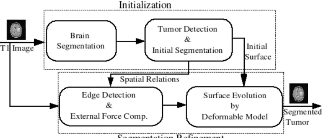
3D brain tumor segmentation in MRI using fuzzy classification, symmetry analysis and spatially constrained deformable models
Texte intégral
Figure


Documents relatifs
Furthermore, we find no evidence for the existence of a substantial popula- tion of quiescent long-lived cells, meaning that the microglia population in the human brain is sustained
Secondary modes can however favor the relevance in the order parameter free energy expansion of higher order terms, which may finally stabilize phases (of lower
Large kidneys predict poor renal outcome in subjects with diabetes and chronic kidney disease?. Vincent Rigalleau, Magalie Garcia, Catherine Lasseur, François Laurent, Michel
Copyright and moral rights for the publications made accessible in the public portal are retained by the authors and/or other copyright owners and it is a condition of
In the last part of the analysis, we used the data from monkey S to compare the spread of activity evoked by sICMS applied in the different body representations of the motor
Keywords: nitric oxide synthase, nitric oxide, nitrosoheme, Staphylococcus xylosus, coagulase-negative Staphylococcus, oxidative
Previous studies performed in patients with severe to mild disorders of consciousness have examined scalp activity in neural sources to search for neural markers
Au cours de l’année universitaire 2001-2002, nous avons eu à l’urgence de l’Hôpital Saint-Luc du CHUM le projet de recherche IMPARCTA : Impact quantitatif et qualitatif de
