HAL Id: hal-02999805
https://hal.archives-ouvertes.fr/hal-02999805
Submitted on 15 May 2021
HAL is a multi-disciplinary open access
archive for the deposit and dissemination of
sci-entific research documents, whether they are
pub-lished or not. The documents may come from
teaching and research institutions in France or
abroad, or from public or private research centers.
L’archive ouverte pluridisciplinaire HAL, est
destinée au dépôt et à la diffusion de documents
scientifiques de niveau recherche, publiés ou non,
émanant des établissements d’enseignement et de
recherche français ou étrangers, des laboratoires
publics ou privés.
Luigi Caputi, Quentin Carradec, Damien Eveillard, Amos Kirilovsky, Eric
Pelletier, Juan Pierella Karlusich, Fabio Rocha Jimenez Vieira, Emilie Villar,
Samuel Chaffron, Shruti Malviya, et al.
To cite this version:
Luigi Caputi, Quentin Carradec, Damien Eveillard, Amos Kirilovsky, Eric Pelletier, et al..
Community-Level Responses to Iron Availability in Open Ocean Plankton Ecosystems. Global
Bio-geochemical Cycles, American Geophysical Union, 2019, 33 (3), pp.391-419. �10.1029/2018GB006022�.
�hal-02999805�
Luigi Caputi1 , Quentin Carradec2,3,4,5 , Damien Eveillard5,6 , Amos Kirilovsky7,8 , Eric Pelletier2,3,4,5 , Juan J. Pierella Karlusich5,7 , Fabio Rocha Jimenez Vieira5,7 , Emilie Villar7,9 , Samuel Chaffron5,6 , Shruti Malviya7,10 , Eleonora Scalco1, Silvia G. Acinas11, Adriana Alberti2,5, Jean‐Marc Aury2 , Anne‐Sophie Benoiston7,12,
Alexis Bertrand2, Tristan Biard9 , Lucie Bittner7,9,12 , Martine Boccara7, Jennifer R. Brum13,14, Christophe Brunet1, Greta Busseni1, Anna Carratalà15, Hervé Claustre16 ,
Luis Pedro Coelho17 , Sébastien Colin5,7,9, Salvatore D'Aniello1 , Corinne Da Silva3,5 , Marianna Del Core18 , Hugo Doré9, Stéphane Gasparini16, Florian Kokoszka1,7,19, Jean‐Louis Jamet20, Christophe Lejeusne1,21 , Cyrille Lepoivre22, Magali Lescot5,23, Gipsi Lima‐Mendez24,25, Fabien Lombard5,16, Julius Lukeš26,27 , Nicolas Maillet1,28 ,
Mohammed‐Amin Madoui2,3,4, Elodie Martinez29 , Maria Grazia Mazzocchi1, Mario B. Néou2,3,4, Javier Paz‐Yepes7, Julie Poulain2,5 , Simon Ramondenc16, Jean‐Baptiste Romagnan30,
Simon Roux14, Daniela Salvagio Manta18, Remo Sanges1, Sabrina Speich5,19 , Mario Sprovieri18, Shinichi Sunagawa17,31 , Vincent Taillandier16 , Atsuko Tanaka7, Leila Tirichine7,32,
Camille Trottier6 , Julia Uitz16, Alaguraj Veluchamy7,33, Jana Veselá26, Flora Vincent7, Sheree Yau34 , Stefanie Kandels‐Lewis17,35, Sarah Searson16 , Céline Dimier7,9, Marc Picheral5,16,Tara Oceans Coordinators, Peer Bork17,35,36,37, Emmanuel Boss38 , Colomban de Vargas5,9,39, Michael J. Follows40, Nigel Grimsley5,34, Lionel Guidi5,16,41 ,
Pascal Hingamp5,23, Eric Karsenti5,7,35, Paolo Sordino1, Lars Stemmann5,16, Matthew B. Sullivan14, Alessandro Tagliabue42 , Adriana Zingone1 , Laurence Garczarek9, Fabrizio d'Ortenzio16, Pierre Testor43 , Fabrice Not9 , Maurizio Ribera d'Alcalà1 , Patrick Wincker2,3,4,5, Chris Bowler5,7 , Daniele Iudicone1
Tara Oceans Coordinators: Silvia G. Acinas11, Peer Bork17,35,36,37, Emmanuel Boss38,
Chris Bowler5,7, Colomban de Vargas5,9,39, Michael J. Follows40, Gabriel Gorsky16, Nigel Grimsley5,34, Pascal Hingamp5,23, Daniele Iudicone1, Olivier Jaillon2,3,
Stefanie Kandels‐Lewis17,35, Lee Karp‐Boss38, Eric Karsenti5,7,35, Uros Krzic44, Fabrice Not9,
Hiroyuki Ogata45, Stéphane Pesant46,47, Jeroen Raes24, Emmanuel G. Reynaud48, Christian Sardet16, Mike Sieracki49,50, Sabrina Speich5,29, Lars Stemmann5,16, Matthew B. Sullivan14,
Shinichi Sunagawa17,31, Didier Velayoudon51, Jean Weissenbach2,3,4, and Patrick Wincker2,3,4,5
1Stazione Zoologica Anton Dohrn, Naples, Italy,2CEA‐ Institut François Jacob, Genoscope, Evry, France,3CNRS UMR,
Evry, France,4Université d'Evry Val d'Essonne, Université Paris‐Saclay, Evry, France,5Research Federation for the Study of Global Ocean Systems Ecology and Evolution, FR2022/GOSEE, Paris, France,6Laboratoire des Sciences du
Numérique de Nantes (LS2N)– CNRS, Université de Nantes, École Centrale de Nantes, IMT Atlantique, Nantes, France,
7Institut de biologie de l'Ecole normale supérieure (IBENS), Ecole normale supérieure, CNRS, INSERM, PSL Université
Paris, Paris, France,8INSERM, UMRS1138, Laboratory of Integrative Cancer Immunology, Centre de Recherche des Cordeliers, Paris, France,9CNRS, Sorbonne Universités, UPMC Univ Paris 06, UMR 7144, Station Biologique de Roscoff,
Place Georges Teissier, Roscoff, France,10Simons Centre for the Study of Living Machines, National Centre for Biological Sciences, Tata Institute of Fundamental Research, Bangalore, India,11Department of Marine Biology and
Oceanography, Institute of Marine Sciences (ICM)‐CSIC, Barcelona, Spain,12Institut de Systématique, Evolution, Biodiversité (ISYEB), Sorbonne Université, Muséum National d'Histoire Naturelle, CNRS, EPHE, Université des Antilles, Paris, France,13Department of Oceanography and Coastal Sciences, Louisiana State University, Baton Rouge, LA, USA,
14Department of Microbiology and Civil, Environmental, and Geodetic Engineering, The Ohio State University,
Columbus, OH, USA,15Laboratory of Environmental Chemistry, School of Architecture, Civil and Environmental Engineering (ENAC), École Polytechnique Fédérale de Lausanne (EPFL), Lausanne, Switzerland,16Sorbonne Université,
CNRS, UMR 7093, Institut de la Mer de Villefranche sur mer, Laboratoire d'Océanographie de Villefranche, Villefranche‐sur‐Mer, France,17Structural and Computational Biology Unit, European Molecular Biology Laboratory,
Heidelberg, Germany,18Institute for Anthropic impacts and Sustainability in the Marine Environment (IAS‐CNR), Capo Granitola, Torretta Granitola, Italy,19LMD Laboratoire de météorologiedynamique. Ecole normale supérieure de Paris,
PSL ResearchUniversity, Paris, France,20CNRS/INSU, IRD, MIO UM 110 Mediterranean Institut of Oceanography,
©2019. American Geophysical Union. All Rights Reserved.
Luigi Caputi, Quentin Carradec, Damien Eveillard, Amos Kirilovsky, Eric Pelletier, Juan J. Pierella, Karlusich, Fabio Rocha Jimenez Vieira, and Emilie Villar contributed equally to this work.
Chris Bowler and Daniele Iudicone equal coordinating contribution.
Key Points:
• Coherent assemblages of taxa covarying with iron at global level are identified in plankton communities
• Functional responses to iron availability involve both changes in copy numbers of iron‐responsive genes and their transcriptional regulation
• Plankton responses to local variations in iron concentrations recapitulate global patterns
Supporting Information: • Supporting Information S1 • Figure S1 • Figure S2 • Figure S3 • Figure S4 • Figure S5 • Figure S6 • Figure S7 • Table S1 • Table S2 • Table S3 Correspondence to:
M. R. d'Alcalà, P. Wincker, C. Bowler, and D. Iudicone, [email protected]; [email protected]; [email protected]; [email protected] Citation:
Caputi, L., Carradec, Q., Eveillard, D., Kirilovsky, A., Pelletier, E., Pierella Karlusich, J. J., et al. (2019). Community‐level responses to iron availability in open ocean plankton ecosystems. Global Biogeochemical Cycles, 33, 391–419. https://doi.org/ 10.1029/2018GB006022
Received 4 JUL 2018 Accepted 17 DEC 2018
Accepted article online 11 JAN 201 Published online 20 MAR 2019
Université de Toulon, Aix Marseille Universités, Université de Toulon, Aix Marseille Universités, La Garde, France,
21Institut Méditerranéen de Biodiversité et d'Ecologie Marine et Continentale (IMBE), UMR 7263 CNRS, IRD, Aix
Marseille Université, Avignon Université, Station Marine d'Endoume, Marseille, France,22Information Génomique et
Structurale, UMR7256, CNRS, Aix‐Marseille Université, Institut de Microbiologie de la Méditerranée (FR3479), ParcScientifique de Luminy, Marseille, France,23CNRS, IRD, MIO, Aix Marseille Univ, Université de Toulon,
Marseille, France,24Department of Microbiology and Immunology, Rega Institute, KU Leuven, Leuven, Belgium,
25VIB, Center for the Biology of Disease, Leuven, Belgium,26Biology Centre CAS, Institute of Parasitology,České
Budějovice, Czech Republic,27Faculty of Science, University of South Bohemia, Ceské Budejovice, Czech Republic,
28USR 3756 IP CNRS, Institut Pasteur‐ Bioinformatics and Biostatistics Hub ‐ C3BI, Paris, France,29University of Brest,
Ifremer, CNRS, IRD, Laboratoire d'Océanographie Physique et Spatiale (LOPS), IUEM, Brest, France,30IFREMER, Physiology and Biotechnology of Algae Laboratory, rue de l'Iled'Yeu, Nantes, France,31Institute of Microbiology,
Department of Biology, Institute of Microbiology and Swiss Institute of Bioinformatics, Zurich, Switzerland,32Faculté des Sciences et Techniques, Université de Nantes, CNRS UMR6286, UFIP, Nantes, France,33Biological and Environmental
Sciences and Engineering Division, King Abdullah University of Science and Technology, Thuwal, Saudi Arabia,
34CNRS, Biologie Intégrative des Organismes Marins (BIOM, UMR 7232), Observatoire Océanologique, Sorbonne
Universités, UPMC Univ Paris 06, Banyuls sur Mer, France,35Directors' Research European Molecular Biology Laboratory Meyerhofstr. 1, Heidelberg, Germany,36Max Delbrück Centre for Molecular Medicine, Berlin, Germany,
37Department of Bioinformatics, Biocenter, University of Würzburg, Würzburg, Germany,38School of Marine Sciences,
University of Maine, Orono, ME, USA,39Sorbonne University, CNRS, Station Biologique de Roscoff, UMR7144,
ECOMAP, Roscoff, France,40Department of Earth, Atmospheric and Planetary Sciences, Massachusetts Institute of Technology, Cambridge, MA, USA,41Department of Oceanography, University of Hawaii, Honolulu, HI, USA, 42Department of Earth Ocean and Ecological Sciences, School of Environmental Sciences, University of Liverpool,
Liverpool, UK,43Laboratoire LOCEAN, Sorbonne Universités (UPMC, Univ Paris 06)‐CNRS‐IRD‐MNHN, Paris, France, 44Cell Biology and Biophysics, European Molecular Biology Laboratory, Heidelberg, Germany,45Institute for Chemical
Research, Kyoto University, Uji, Kyoto, Japan,46MARUM, Center for Marine Environmental Sciences, University of
Bremen, Bremen, Germany,47PANGAEA, Data Publisher for Earth and Environmental Science, University of Bremen, Bremen, Germany,48Earth Institute, University College Dublin, Dublin, Ireland,49National Science Foundation,
Arlington, VA, USA,50Bigelow Laboratory for Ocean Sciences East Boothbay, Boothbay, ME, USA,51DVIP Consulting, Sèvres, France
Abstract
Predicting responses of plankton to variations in essential nutrients is hampered by limited in situ measurements, a poor understanding of community composition, and the lack of reference gene catalogs for key taxa. Iron is a key driver of plankton dynamics and, therefore, of global biogeochemical cycles and climate. To assess the impact of iron availability on plankton communities, we explored the comprehensive bio‐oceanographic and bio‐omics data sets from Tara Oceans in the context of the iron products from two state‐of‐the‐art global scale biogeochemical models. We obtained novel information about adaptation and acclimation toward iron in a range of phytoplankton, including picocyanobacteria and diatoms, and identified whole subcommunities covarying with iron. Many of the observed global patterns were recapitulated in the Marquesas archipelago, where frequent plankton blooms are believed to be caused by natural iron fertilization, although they are not captured in large‐scale biogeochemical models. This work provides a proof of concept that integrative analyses, spanning from genes to ecosystems and viruses to zooplankton, can disentangle the complexity of plankton communities and can lead to more accurate formulations of resource bioavailability in biogeochemical models, thus improving our understanding of plankton resilience in a changing environment.Plain Language Summary
Marine phytoplankton require iron for their growth and proliferation. According to John Martin's iron hypothesis, fertilizing the ocean with iron coulddramatically increase photosynthetic activity, thus representing a biological means to counteract global warming. However, while there is a constantly growing knowledge of how iron is distributed in the ocean and about its role in cellular processes in marine photosynthetic groups such as diatoms and cyanobacteria, less is known about how iron availability shapes plankton communities and how they respond to it. In the present work, we exploited recently published Tara Oceans data sets to address these questions. Wefirst defined specific subcommunities of co‐occurring organisms that co‐vary with iron availability in the oceans. We then identified specific patterns of adaptation and acclimation to iron in different groups of
phytoplankton. Finally, we validated our global results at local scale, specifically in the Marquesas archipelago, where recurrent phytoplankton blooms are believed to be a result of iron fertilization. By
integrating global data with a localized response, we provide a framework for understanding the resilience of plankton ecosystems in a changing environment.
1. Introduction
Marine plankton play critical roles in pelagic oceanic ecosystems. Their photosynthetic component (phyto-plankton, consisting of eukaryotic phytoplankton and cyanobacteria) accounts for approximately half of Earth's net primary production, fueling marine food webs, and sequestration of organic carbon to the ocean interior. Phytoplankton stocks depend on the availability of primary resources such as nutrients that are characteristically limiting in the oligotrophic ocean. For example, high‐nutrient low‐chlorophyll (HNLC) regions are often lacking the key micronutrient iron and increased bioavailability of iron will typically trig-ger a phytoplankton bloom (Boyd et al., 2007). Notwithstanding, the community response and its impact on food web structure and biogeochemical cycles are seldom predictable. The composition of blooms when lim-iting nutrients are supplied as sudden pulses with respect to the pre‐existing community has been only poorly explored and is even more elusive when comparing to situations when nutrients are in quasi‐steady state. Characterizing these responses is crucial to anticipate future changes in the ocean yet is challenged by community complexity and processes that span from genes to ecosystems. Dissecting these processes would also enhance the robustness of existing biogeochemical models and improve their predictive power (Stec et al., 2017).
In this report we explore the responsiveness of plankton communities to iron and assess the representation of iron bioavailability in biogeochemical models. Using global comprehensive metagenomics and metatran-scriptomics data from Tara Oceans (Alberti et al., 2017; Bork et al., 2015; Carradec et al., 2018; Guidi et al., 2016), we examine abundance and expression profiles of iron‐responsive genes in diatoms and other phyto-plankton, together with clade composition in picocyanobacteria and the occurrence of iron‐binding sites in bacteriophage structural proteins. These profiles are compared in the global ocean with the iron products from two state‐of‐the‐art biogeochemical models. We further identify coherent subcommunities of taxa cov-arying with iron in the open ocean that we denote iron‐associated assemblages (IAAs). Overall, our findings are congruent with the outputs from the models and reveal a range of adaptive and acclimatory strategies to cope with iron availability within plankton communities. As a further proof of concept, we track community composition and gene expression changes within localized blooms downstream of the Marquesas archipe-lago in the equatorial Pacific Ocean, where previous observations have suggested them to be triggered by iron (Martinez & Maamaatuaiahutapu, 2004), even though the biogeochemical models currently lack the resolution to detect the phenomenon. Our results indicate that iron does indeed drive the increased produc-tivity in this area, suggesting that a pulse of the resource can elicit a response mimicking global steady state patterns.
2. Materials and Methods
2.1. Iron Concentration EstimatesDue to the sparse availability of direct observations of iron in the surface ocean, iron concentrations were derived from two independent global ocean simulations. Thefirst is the ECCO2‐DARWIN ocean model con-figured with 18‐km horizontal resolution and a biogeochemical simulation that resolves the cycles of nitro-gen, phosphorus, iron, and silicon (Menemenlis et al., 2008). The simulation resolves 78 virtual phytoplankton phenotypes. The biogeochemical parameterizations, including iron, are detailed in Follows et al. (2007). In brief, iron is consumed by primary producers and exported from the surface in dissolved and particulate organic form. Remineralization fuels a pool of total dissolved iron, which is partitioned between free iron and complexed iron, with afixed concentration and conditional stability of organic ligand. Scavenging is assumed to affect only free iron, but all dissolved forms are bioavailable. Atmospheric deposi-tion of iron was imposed using monthlyfluxes from the model of Mahowald et al. (2005).
PISCES (Aumont et al., 2015) is a more complex global ocean biogeochemical model than ECCO2‐ DARWIN, representing two phytoplankton groups, two zooplankton grazers, two particulate size classes, dissolved inorganic carbon, dissolved organic carbon, oxygen, and alkalinity, as well as nitrate, phosphate, silicic acid, ammonium, and iron as limiting nutrients. In brief, PISCES accounts for iron inputs from
dust, sediments, rivers, sea ice, and continental margins, andflexible Michaelis‐Menten‐based phytoplank-ton uptake kinetics result in dynamically varying iron stoichiometry and drives variable recycling by zoo-plankton and bacterial activity. Iron loss accounts for scavenging onto sinking particles as a function of a prognostic iron ligand model, dissolved iron levels, and the concentration of particles. Iron loss from colloi-dal coagulation is also included and accounts for both turbulent and Brownian interactions of colloids. The PISCES iron cycle we use is denoted as“PISCES2” (Tagliabue et al., 2016) performed at the upper end of a recent intercomparison of 13 global ocean models that included iron.
2.2. In Situ Data
To generate a limited data set of observed dissolved iron concentrations for this analysis, we used a dissolved iron database updated from Tagliabue et al. (2012). For this we searched for the nearest available observation at the same depth as the Tara Oceans sampling and collected data that were within a horizontal radius of 2° from the sampling coordinates.
2.3. Marquesas Archipelago Sampling
Four stations within the Marquesas archipelago were sampled during the Tara Oceans expedition in August 2011 (Bork et al., 2015) using protocols described in Pesant et al. (2015): They were denoted TARA_122, TARA_123, TARA_124, and TARA_125. The sample details and physicochemical parameters recorded dur-ing the cruise are available at PANGAEA (http://www. pangaea.de), and nucleotide data are accessible at the ENA archive (http://www.ebi.ac.uk/ena/) (see further details below).
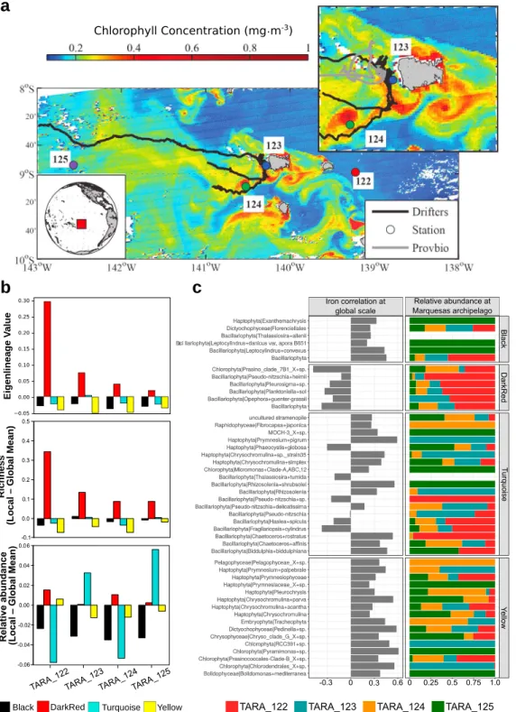
The study was initiated by releasing a glider that characterized the water column until the end of the experi-ment. First, the mapping of the water column structure via real‐time analysis of glider data was conducted. After this initial step, the continuous inspection of near real‐time satellite color chlorophyll images and alti-metric data revealed a highly turbulent environment, with a mixed layer up to 100‐m deep and strong lateral shearing, especially downstream of the islands, which generated an area of recirculation in the wake of the main island (Nuku Hiva). A series of four sampling stations was then planned and executed by performing the full set of measurements and sampling using the Tara Oceans holistic protocol (Pesant et al., 2015). Station TARA_122 sampled the HNLC prebloom waters upstream of the islands and thus served as a refer-ence station for the others. This station was located 27‐km upstream of the island of Nuku Hiva.
2.4. Oceanographic Observations
The Biogeochemical Argofloat deployed in the framework of the Marquesas study (WMO 6900985) was a PROVBIO‐1 free‐drifter profiler (Xing et al., 2012). It was based on the “PROVOR‐CTS3” model, equipped with a standard CTD sensor (to retrieve temperature and salinity parameters) together with bio‐optical sen-sors for the estimation of chlorophyll‐a concentrations, colored dissolved organic matter, and backscatter at 700 nm. It was also equipped with a radiometric sensor to estimate spectral downward irradiance at three wavelengths (412, 490, and 555 nm) and with a beam transmissometer. The data processing is discussed in Xing et al. (2012). The profiling float was programmed to adopt a modified standard Argo strategy (Freeland & Cummins, 2005). After deployment, it navigated at 700‐m depth, to a daily maximum of 1,000 m, and then surfaced afirst time, generally early in the morning. It then submerged again to a depth up to 400 m, to again reach the surface approximately at noon. A third profile to 400 m, followed by a sub-sequent resurfacing, was performed at the end of the day. During all the ascending phases, a complete profile of all the available parameters was collected. At surface, the obtained data were transmitted to land through a satellite connection and the profiler descended again to 1,000 m to start another cycle. The Biogeochemical Argo was deployed on‐site at Station TARA_123 on 2 August 2011. It performed 55 profiles in the Marquesas region, before moving westward in early October (then outside the study area), and then southward. It de fi-nitively ceased to function in December 2012, approximately 400 km south of the Marquesas islands and after collecting more than 150 profiles.
An autonomous glider was also deployed in the study area. A complete description of glider technology and functioning is available in Testor et al. (2010). This glider was able to reach 1,000‐m depths. It was equipped with temperature and salinity sensors, an optode for oxygen concentration measurements, two Wetlab eco-pucks with twofluorometers for chlorophyll and colored dissolved organic matter concentrations, and three backscatterometers to estimate backscatter coefficients at three wavelengths (532, 700, and 880 nm). The gli-der was deployed on 16 July 2011 (approximately 1 month before TARA arrived in the Marquesas
archipelago), close to the position of Station TARA_122. It was recovered on 5 August 2011 by TARA because a malfunction in the tail rudder had been detected. It performed approximately 250 profiles, with 35 dives at 1,000‐m depths and 90 dives at 500‐m depths.
Analysis of trace metals was performed exclusively at the Marquesas Islands sampling stations (Stations TARA_122‐TARA_125) following the methods reported in Scelfo (1997). Dissolved iron was not measured due to lack of technical resources.
2.5. Network Analysis and Correlations With Iron
A co‐occurrence network analysis similar to that reported in Guidi et al. (2016) was performed to delineate feature subnetworks of prokaryotic and eukaryotic lineages, as well as viral populations, based on their rela-tive abundance. All procedures were applied on 103 sampling sites (Guidi et al., 2016) after excluding out-liers (Stations TARA_82, TARA_84 and TARA_85) on Hellinger‐transformed log‐scaled abundances. Computations were carried out using the R package WGCNA (Langfelder & Horvath, 2007). After building a co‐occurrence weighted graph, a hierarchical clustering was performed. This resulted in the definition of several subnetworks or modules, each represented by itsfirst principal component, called module eigen value. Associations between the calculated subnetworks and a given trait were measured by the pairwise Pearson correlation coefficients, as well as with corresponding p values corrected for multiple testing using the Benjamini and Hochberg false discovery rate (FDR) procedure, between the considered environmental trait and their respective principal components. The results are reported in thefirst 10 columns of the heat-map in Figure S1a in the supporting information. The subnetworks that showed the highest correlation scores are of interest to emphasize a putative community associated with a given environmental trait. In addition to the multiple environmental parameters previously reported (Guidi et al., 2016), we simulated iron bioavailability in Tara Oceans stations based on the two different models of iron concentration in the global oceans: the ECCO2‐DARWIN model (Menemenlis et al., 2008) and the PISCES2 model (Aumont et al., 2015). Both models performed well in the recent global iron model intercomparison project (Tagliabue et al., 2016), and so we conducted an assessment of model outputs at Tara Oceans sampling loca-tions using compilaloca-tions of iron observaloca-tions (Tagliabue et al., 2016) augmented by those from the GEOTRACES program (Mawji et al., 2014). ECCO2‐DARWIN‐derived estimates (57 stations at surface) and PISCES2 model (83 stations at surface, 44 of which also at maximum chlorophyll depth) can be found in Table S1a. For further details on the models and for a comparison of the two, see the supporting information. We then identified eukaryotic, prokaryotic, and viral subnetworks that correlated most strongly with iron bioavailability, denoted IAAs. Four IAAs consisting of eukaryotic metabarcodes (de Vargas et al., 2015) were significantly associated with iron. Similarly, four viral IAAs could be identified by analysis of viral commu-nities. Based on taxonomy, no prokaryotic IAAs with significance could be identified; however, when con-sidering prokaryotic genes (as described in Guidi et al., 2016),five subnetworks of prokaryotic genes could be identified.
In addition to the network analyses, we examined whether the identified subnetworks can be used as predic-tors of iron bioavailability. Following the protocol described in Guidi et al. (2016), we used partial least square regression, which is a dimensionality‐reduction method that aims to determine predictor combina-tions with maximum covariance with the response variable. The predictors were ranked according to their value importance in projection(VIP) using the R package pls (Mevik & Wehrens, 2007). For each eukaryotic IAA, their relative contribution to each sample was estimated by computing thefirst eigen value.
2.6. Taxonomy Determinations
Taxonomic studies were performed using various methods (photosynthetic pigments,flow cytometry, and optical microscopy for phytoplankton and zooplankton as detailed in Villar et al. (2015); phytoplankton counts using unfiltered bottles or nets as described in Malviya et al. (2016) and Villar et al. (2015); and meso-zooplankton samples collected by vertical tows with a WP2 net (200‐μm mesh aperture) from 100‐m depth to the surface during the day, followed byfixation in buffered formaldehyde (2–4% final concentration), and later analyzed in the laboratory). Data from an Underwater Vision Profiler (UVP) were used to determine particle concentrations and size distributions >100μm, (Campbell et al., 1994). To have an estimate of bio-mass variations in the different compartments at the Marquesas Islands, we applied empirical formulas to transform Chlorophyll‐a (phytoplankton) or body measurements (zooplankton) to biomass. To this
purpose, we used the ratio of phytoplankton biomass to Chlorophyll‐a (Phyto C: Chl a) in the euphotic zone as previously estimated in an area with similar biogeochemical features (Campbell et al., 1994—See Table S1b). Of note, our aim was not to determine absolute biomass but to estimate variations in biomass between the Marquesas Islands stations. To estimate the total phytoplankton biomass, Chl a concentration from HPLC data was thus used. The relative contribution of microplankton, nanoplankton, and picoplankton to the [Chla]totwas estimated according to Uitz et al. (2006). The biomass of large zooplankton was
esti-mated using previously published conversion factors from body length to carbon content (C:L) in selected zooplankton lineages. Individual body measures were estimated from literature considering similar commu-nity composition, with the exception of the Copepoda prosome length, which was herein measured. Zooscan (Bongo net, >300μm) derived abundance data (ind × m−3) were used to evaluate the total biomass along the water column.
2.7. Genomic Analyses
Eukaryotes larger than 5μm were collected directly from the ocean using nets with different mesh sizes while smaller organisms and viruses were sampled by peristaltic pump followed by on‐deck filtration. Severalfiltration steps were performed using membranes with different pore sizes to obtain size‐fractionated samples corresponding to viruses (<0.1 and 0.1–0.2 μm), prokaryotes (0.2–3 μm), and eukaryotes (0.8–5, 5–20, 20–180, and 180–2,000 μm). In this study, we only used samples collected from the surface water layer. Details about genomics methods are available in Carradec et al. (2018) and in the following publications: virus metagenomes (Roux et al., 2016); prokaryote metagenomes (Sunagawa et al., 2015); eukaryote metabarcoding (de Vargas et al., 2015); and eukaryote metagenomes and metatranscriptomes (Alberti et al., 2017; Carradec et al., 2018). The abundance of individual genes was assessed by normaliza-tion to the total number of sequences within the same organismal group (Carradec et al., 2018). Cyanobacterial clade absolute cell abundance was assessed using the petB marker gene, as described in Farrant et al. (2016), in combination with flow cytometry counts using the method published by Vandeputte et al. (2017).
Metatranscriptomic and metagenomic unigenes were functionally annotated using PFAM (Finn et al., 2016) as the reference database and search tool (Katoh & Standley, 2013). To detect the presence of genes encoding silicon transporters, ferritin, proteorhodopsin, FBAI, and FBAII among the unigene collection, the profile hidden Markov models of the PFAMs PF03842, PF0210, PF01036, PF00274, and PF01116, respectively, were used, with HMMer v3.2.1 with gathering threshold option (http://hmmer.org/). It is important to note that flavodoxin (PF00253, PF12641, and PF12724), ferredoxin (PF00111), and cytochrome c6(PF13442) PFAM
families do not discriminate those sequences involved in photosynthetic metabolism from other homologous sequences. The photosynthetic isoforms forflavodoxin, ferredoxin, and cytochrome c6were therefore
deter-mined by phylogeny, as described below.
To discriminate the photosynthetic isoforms from other homologous sequences, we started with the results from HMMer and then built libraries composed of well‐known reference sequences (manually and experimentally curated) from both photosynthetic and nonphotosynthetic pathways. To enrich our libraries, we used the reference sequences to find similar sequences by using BLAST search tool (“tBLASTn” program with an e−5e value threshold) against phyloDB reference database (Dupont et al., 2015). Next, we used MAFFT version 7 using the G‐INS‐I strategy (Katoh & Standley, 2013). The corre-sponding phylogenetic reference trees were generated with PhyML 3.0 (Guindon et al., 2010) using the LG substitution model with four categories of rate variation. The starting tree was a BIONJ tree, and the type of tree improvement was subtree pruning and regrafting. Branch support was calculated using the approximate likelihood ratio test with a Shimodaira‐Hasegawa‐like procedure. We then manually identified the branches containing the photosynthetic versions and those with nonphotosynthetic pro-teins. We ensured that the approximate likelihood ratio test values of the photosynthetic and nonphoto-synthetic branches were higher than 0.7 by retaining only the most conserved matches in our trees. Finally, we realigned and labeled the unigenes against the reference trees depending on the placement of each translated unigene on them.
While HMMer has the highest sensitivity among the classical domain detection approaches, not all the refer-ences collected by PFAM are sufficiently rich with HMMer to maintain the same detection (Bernardes et al.,
2016). To deal with the poor representation of ISIP genes in the PFAM database and to improve their detection, we adopted a simplified version of the approach presented in Bernardes et al. (2015) to build our own pHMM to detect the different conserved regions represented by ISIP1, ISIP2a, and ISIP3 amino acid sequences. For this, we collected all the sequences in the reference literature (Allen et al., 2008; Chappell et al., 2015; Lommer et al., 2010; Morrissey et al., 2015), all 35 sequences belonging to PFAM PF07692 and the 56 most conserved sequences from PF03713 (all the seeds).
2.8. Data and Code Availability
Sequencing data are archived at ENA under the accession number PRJEB4352 for the metagenomics data and PRJEB6609 for the metatranscriptomics data (Carradec et al., 2018). Environmental data are available at PANGAEA. The gene catalog, unigene functional and taxonomic annotations, and unigene abundances and expression levels are accessible at http://www.genoscope.cns.fr/tara/. Computer codes are available upon request to the corresponding authors.
2.8.1. Accession Numbers of Metagenomics and Metatranscriptomics Data 2.8.1.1. Sample
ERS492651, ERS492651, ERS492650, ERS492669, ERS492669, ERS492662, ERS492662, ERS492658, ERS492658, ERS492650, ERS492740, ERS492742, ERS492742, ERS492751, ERS492751, ERS492763, ERS492763, ERS492757, ERS492740, ERS492757, ERS492825, ERS492825, ERS492824, ERS492824, ERS492829, ERS492852, ERS492852, ERS492846, ERS492846, ERS492829, ERS492897, ERS492897, ERS492895, ERS492895, ERS492912, ERS492912, ERS492909, ERS492909, ERS492904, ERS492904.
2.8.1.2. Experiment
ERX948080, ERX948010, ERX1782415, ERX1782384, ERX1782327, ERX1796912, ERX1796638, ERX1796690, ERX1796805, ERX1782126, ERX1782109, ERX1782245, ERX1796854, ERX1796544, ERX1782292, ERX1782172, ERX1782221, ERX1796700, ERX1796855, ERX1782301, ERX1782464, ERX1782128, ERX1789668, ERX1789366, ERX948029, ERX948074, ERX1796627, ERX1796773, ERX1789369, ERX1789449, ERX1796931, ERX1796605, ERX1789426, ERX1789575, ERX1789524, ERX1796866, ERX1796524, ERX1789649, ERX1789612, ERX1789647, ERX1796596, ERX1796836, ERX1789655, ERX1789574, ERX1789407, ERX1782118, ERX1782283, ERX947973, ERX948088, ERX1789391, ERX1789539, ERX1789587, ERX1796687, ERX1796586, ERX1796703, ERX1789662, ERX1789616, ERX1789589, ERX1796662, ERX1796518, ERX1796678, ERX1796698, ERX1782217, ERX1782352, ERX1796645, ERX1796858, ERX1796924, ERX1789675, ERX1789597, ERX1789700, ERX1789362, ERX1782350, ERX1782418, ERX947994, ERX948064, ERX1789361, ERX1789368, ERX1789532, ERX1796658, ERX1796818, ERX1796632, ERX1789638, ERX1789548, ERX1789579, ERX1796921, ERX1796732, ERX1796741, ERX1789714, ERX1789489, ERX1789628, ERX1796689, ERX1796850, ERX1796523, ERX1782181, ERX1782370, ERX1796607, ERX1796738, ERX1796714, ERX1789437, ERX1789516, ERX1789417.
2.8.1.3. Run
ERR868475, ERR868513, ERR1712182, ERR1712118, ERR1711869, ERR1726556, ERR1726667, ERR1726938, ERR1726688, ERR1712207, ERR1711933, ERR1711897, ERR1726927, ERR1726932, ERR1712069, ERR1712197, ERR1711986, ERR1726883, ERR1726891, ERR1712219, ERR1711929, ERR1711951, ERR1719463, ERR1719159, ERR868466, ERR868469, ERR1726762, ERR1726913, ERR1719393, ERR1719310, ERR1726961, ERR1726522, ERR1719437, ERR1719413, ERR1719343, ERR1726622, ERR1726721, ERR1719297, ERR1719410, ERR1719307, ERR1726770, ERR1726561, ERR1719256, ERR1719298, ERR1719217, ERR1711914, ERR1711917, ERR868363, ERR868489, ERR1719301, ERR1719160, ERR1719214, ERR1726564, ERR1726725, ERR1726569, ERR1719448, ERR1719389, ERR1719194, ERR1726571, ERR1726533, ERR1726892, ERR1726601, ERR1711949, ERR1712155, ERR1726608, ERR1726657, ERR1726763, ERR1719391, ERR1719175, ERR1719381, ERR1719365, ERR1711882, ERR1711999, ERR868382, ERR868352, ERR1719395, ERR1719316, ERR1719207, ERR1726643, ERR1726714, ERR1726846, ERR1719404, ERR1719213, ERR1719459, ERR1726822, ERR1726912, ERR1726691, ERR1719356, ERR1719145, ERR1719293, ERR1726695, ERR1726666, ERR1726903, ERR1712102, ERR1711923, ERR1726745, ERR1726946, ERR1726765, ERR1719295, ERR1719249, ERR1719385.
3. Results
3.1. Modeled Iron Distributions Are Highly Correlated With the Expression of Marker Genes for Iron Limitation
Iron is a complex contamination‐prone micronutrient whose bioavailability is difficult to assess in the ocean (Tagliabue et al., 2017). Rather than using single discrete measurements, we linked observed differences in plankton communities at sites sampled during the Tara Oceans expedition (Bork et al., 2015) with the range of iron conditions typical of each location. Specifically, we extracted annual mean iron concentrations and their variability from two state‐of‐the‐art ocean models (ECCO2‐DARWIN [Menemenlis et al., 2008] and PISCES2 [Aumont et al., 2015]) and analyzed their correspondence with the best available estimates based upon in situ data (a compilation of iron observations [Tagliabue et al., 2012] merged with GEOTRACES data [Mawji et al., 2014; Tagliabue et al., 2012] in a manner similar to previous studies [Toulza et al., 2012]; Figure 1).
To assess the reliability of the modeled iron distributions, we correlated the expression of diatom ISIP genes in metatranscriptomics data sets with the annual means of iron concentrations estimated by the DARWIN model, and with annual and monthly means by the PISCES2 model (Carradec et al., 2018; Table S1a and supporting information S1). These genes have been found in multiple previous studies to be inversely corre-lated with iron availability (Allen et al., 2008; Chappell et al., 2015; Graff van Creveld et al., 2016; Marchetti et al., 2017; Morrissey et al., 2015). Figure 1 presents a comparison between the estimates of dissolved iron concentrations derived from the annual mean ironfield from PISCES2 and ECCO2‐DARWIN (Table S1a), with the Tara Oceans stations superimposed and best available estimates based upon in situ
Figure 1. Comparison of ECCO2‐DARWIN and PISCES2 iron estimates with observed data and expression of diatom ISIP genes at Tara Oceans stations. Maps of (a) annual average iron concentrations from the ECCO2‐DARWIN model (57 stations at surface), (b) from the PISCES2 model (83 stations at surface, 44 of which also at deep chlorophyll maximum depth), and (c) from the observed data where it was available at less than 2° radius distance from locations of the Tara Oceans sampling sites (20 stations at surface, 16 of which also at deep chlorophyll maximum depth). Each circle corresponds to a sampling site, where the upper semicircle isfilled according to the surface iron concentration while the lower semicircle is filled according to the deep chlorophyll maximum depth where available. Color scale indicates dissolved iron concentrations expressed in nM. (d) Biogeographical pattern of diatom ISIP gene expression. The circle colors represent iron concentration estimates at each Tara Oceans sampling site according to PISCES2 model (Table S1a). The abundance of ISIP transcripts was normalized by the total abundance of all diatom unigenes at each station, and the corresponding values are represented by the circle area. Boxes indicate the Marquesas Islands sampling area.
measurements (Figure 1). In spite of the evident scarcity of actual iron concentration data (which illustrates the need to use models for estimating iron in the current exercise; Figure 1), both models and ISIP mRNA levels describe very satisfactorily the global‐scale gradients, with the highest concentrations of iron observed in the Mediterranean and Arabian Seas (both highly impacted by desert dust deposition) and the lowest in the tropical Pacific and Southern Oceans. This demonstrates that the geographical coverage of the Tara Oceans expedition is well suited to studies of the role of iron on euphotic planktonic ecosystems. The avail-able data (Figure 1; Tavail-able S1a) further indicates that the gradients of iron appear to be better captured by PISCES2, a more complex and recent model (Aumont et al., 2015). This is for instance the case for the North Atlantic Ocean and the Mediterranean Sea, where longitudinal gradients are stronger in PISCES2 and are consistent with ISIP gene levels, while ECCO2‐DARWIN seems to overestimate iron in the Eastern Atlantic Ocean and underestimate it in the Mediterranean Sea. The opposite is true in the South Atlantic Ocean, where ISIP mRNA levels show a clear increase correlated with iron stress between South America and Africa (Figure 1). Overall, in the Atlantic ECCO2‐DARWIN has higher concentrations, and thus, a clearer large‐scale Atlantic‐Pacific gradient is observed.
The Pacific and Southern Oceans (subpolar and polar stations TARA 81–85) are both characterized by low levels of iron, as mentioned above. Notably, PISCES2 has a ratherflat distribution in the Pacific Ocean, with very low values, while the other model shows a relatively higher level of iron at the core of the subtropical gyres, that is, close to the Hawaii Islands (Stations TARA_131 and TARA_132) and offshore from South America (TARA_98 and close‐by stations) that seems to be in agreement with ISIP mRNA levels (at least for the Hawaiian sample—Figure 1). These are very oligotrophic oceanic regions, where nitrate is also a strongly limiting nutrient. Again, the ISIP expression pattern in Figure 1 is closer to the PISCES2 model, in that it shows a clear reduction of the stress resulting from iron deprivation within these gyres. Finally, while a significant increase in iron at the Equator may be expected as a consequence of the upwelling in this region, both the models and the ISIP levels (at Station TARA_128) suggest that this area is rather character-ized by low values of iron. Overall, our analysis indicates that both models correlated very well with Tara Oceans transcriptomic data, with no relevant differences among monthly and yearly values, but with annual means from the ECCO2‐DARWIN estimates showing the best reliability (Table S1c). This analysis also indi-cates that metatranscriptomics is now mature enough to provide an independent, biologically based valida-tion of ecosystem models.
3.2. Plankton Response to Iron Availability Is Coordinated at Subcommunity Level
The higher level organization of plankton communities, and its possible relationship with the roles of indi-vidual constituents, has been highlighted previously in an analysis of the potential links between commu-nity structure and carbon export using data from Tara Oceans (Guidi et al., 2016). We here used this approach to explore plankton ecosystem responses to iron bioavailability using an end‐to‐end approach from genes to communities and from viruses to metazoa to reveal community responses at global scale (see section 2). Known as weighted gene correlation network analysis (WGCNA; see section 2 for further descrip-tion; Guidi et al., 2016; Langfelder & Horvath, 2007), this approach deciphers subcommunities (modules) of organisms within a global co‐occurrence network, and because of the high levels of covariation of individual taxa, it is possible to deduce putative ecological interactions. As proxies for organism abundance we used the relative abundances of eukaryotic lineages (defined as operational taxonomic units; OTUs) derived from 18S‐V9 rDNA metabarcoding data (de Vargas et al., 2015). WGCNA generated a total of 31 modules. Each module groups a subset of eukaryotic taxa found in Tara Oceans samples whose pairwise relative abundance was highly correlated over all the sampling sites; that is, they have a high probability of co‐occurrence and to change their abundance in a coordinated way. Because they react in phase, we can infer that within each subcommunity these organisms have a higher probability of interaction among themselves than with the organisms in other modules.
We found four eukaryotic subnetworks significantly associated with the ECCO2‐DARWIN‐derived and/or with the PISCES2‐derived estimates of iron concentrations in the global ocean (Figures 2a, S1a, and S1b; Table S1d). The Black and Turquoise modules were associated with high significance to the iron concentra-tions generated by both models whereas the DarkRed and Yellow modules were better associated with ECCO2‐DARWIN and PISCES2, respectively, Black (DARWIN: R = 0.37, P = 6 × 10⁻⁴; PISCES2: R= 0.38, P = 3 × 10⁻⁴), Turquoise (DARWIN: R = 0.46, P = 1 × 10⁻⁵; PISCES2: R = 0.42, P = 9 × 10⁻⁵),
DarkRed (DARWIN: R =−0.43, P = 5 × 10⁻⁵; PISCES2: R = 0.19, P = 0.08), and Yellow (DARWIN: R = 0.19, P= 0.09; PISCES2: R = 0.56, P = 5 × 10⁻⁸), and contained between 31 and 591 different OTUs (Tables S1d and S1e). These subnetworks were denoted IAAs. For each IAA subnetwork, WGCNA computes a single representative as a combination of lineages. Such a score, denoted as“module eigengene” score (hereafter termed an eigenlineage score), represents thefirst eigenvector of the assemblage (Langfelder & Horvath, 2007). Projections of samples on such an eigenvector show the relative importance of samples to the global variance of each IAA. Together with their contribution, in terms of OTU abundance to the total eukaryotic abundance in each station (Table S1f), they provide clues to interpret the link between modules and iron availability. The mismatch in some regions between the two models (see above) is likely the reason why the significance of association of the Yellow module with ECCO2‐DARWIN, whose variance and representativeness is particularly significant in the South Adriatic and is minimally present in the Peruvian upwelling area, is much less than that with PISCES2. By contrast, the DarkRed module, which appears to be the best indicator module for the Marquesas area (Figure 2b, upper panel) and is highly relevant in the Peruvian upwelling region, displays a much less significant association and an opposite variation with PISCES2 iron versus ECCO2‐DARWIN iron. The IAAs show slightly different, often antagonistic, variance contributions at global scale (Figure 2b, upper panel), with each of them being particularly responsive, in terms of variance, in specific sites, for example, the Yellow module in the Eastern Mediterranean Sea.
Figure 2. Planktonic iron‐associated assemblages (IAAs) in the global ocean and in the Marquesas Islands stations. (a) Description of eukaryotic modules associated with iron. Relative abundances and co‐occurrences of eukaryotic lineages were used to decipher modules. Four modules can predict iron with high accuracy: Black, DarkRed, Turquoise, and Yellow. For each IAA, lineages are associated to their score of centrality (x‐axis), to their correlation with iron concentrations (y‐axis), and their VIP score (circle area). Representative lineages within each module are emphasized by circles and named (C = Copepoda; B = Bacillariophyta; R = Rhizaria). (b) Upper panel: contribution of Tara Oceans stations to the global variance of IAAs of eukaryotic lineages. For each IAA, we represent the projection of stations on thefirst principal component (upper panel). Lower panel: projection of the relative contribution of the Tara Oceans stations to the global variance of iron‐associated prokaryotic gene assemblages, as revealed by WGCNA. For each prokaryotic gene module associated with iron (from top to bottom: Grey60, Plum1, Red, SkyBlue, and SaddleBrown), we represent the projection of stations on thefirst principal component, proportional to triangle sizes for each module. The behavior of each IAA in the Marquesas archipelago stations is shown in the inset.
We examined the lineage composition of each IAA and the relevance of each taxon within them by deter-mining the relative abundance of each lineage with respect to iron concentration estimates and their central-ity within the module (see section 2). The results are reported in Tables S1d and S1e. The IAAs displayed significant differences in terms of numbers of lineages and compositions, with the Turquoise module being the largest and dominated by consumers, predominantly metazoans, and the DarkRed module being the smallest. The Black module displayed the highest proportion of autotrophs, while the DarkRed IAA dis-played the highest proportion of diatoms (Bacillariophyta; 57% of all autotrophic protists).
To reduce complexity further, we screened the networks in terms of the VIP score of each node (i.e., the OTUs displaying the highest statistical weight in differentiating sites because of iron availability; section 2; Table S1d; Figures 2a and S1c). Species with high VIP scores can be predicted to be particularly important in reflecting the adjustments of each module via their specific interactions with other members of their subcommunity. Although interpreting why high VIP taxa are related to iron bioavailability is often severely restricted by our knowledge of plankton functional ecology and interorganism interactions, in other cases the role of VIP taxa within the modules is clearer. As an example, identification of an IAA in which several diatoms have the highest VIPs (DarkRed module, eight subnetwork members,−0.337 correlation with iron), commonly found in the most severely iron‐limited regions of the world's ocean and often the most responsive groups in mesoscale iron fertilization experiments (Boyd et al., 2007; Marchetti et al., 2006), suggests a strong physiological plasticity of these groups (Greene et al., 1991; Lommer et al., 2012). The fact that Pseudo‐nitzschia is among the highest scoring VIP genera in the DarkRed module further suggests that this genus tracks regions with low iron bioavailability, being able to profit from it when it becomes available. Other examples concern metazoans: copepods from the genus Temora(high subnetwork centrality and strong correlation with iron) are known to be iron‐limited (Chen et al., 2011), and the two cnidarian lineages—the class Hydrozoa and the genus Pelagia (both of which display relatively strong subnetwork centrality and strong correlations with iron)—suggest strong predator‐prey links.
Considering the ECCO2‐DARWIN‐derived VIP scores, lineages with the highest scores (>1) could predict as much as 61.9%, 52.6%, 49.1%, and 38.1% (in the Turquoise, Black, DarkRed, and Yellow IAAs, respectively; leave‐one‐out cross‐validated) of the variability of iron in the oligotrophic ocean. When the PISCES2‐derived VIP scores are taken into account, the predictive potential of the IAAs is even higher: 73.2% (Turquoise), 61.9% (Yellow), 59.0% (Black), and 54.4% (DarkRed). More importantly, the VIP scores obtained with the two models for each OTU showed an extremely good covariance (Figure S1d). This confirms the biological coherence and stability of the modules and their components to iron availability despite the occasional mis-match in the predictions of the two models.
Of the photosynthetic groups, autotrophic dinoflagellate taxa were particularly relevant in the Turquoise and Black modules, diatoms were relevant in the DarkRed module, and haptophytes were significantly pre-sent in the Yellow module. Metazoans were particularly important in the Black and the Turquoise modules, and marine stramenoplies/marine alveolata groups of phagotrophic and parasitic heterotrophs were rele-vant in the Black (marine alveolata), Turquoise, and Yellow modules (marine stramenoplies; Figures 2a and S1c; Tables S1d and S1e). This hints at particularly intricate, and still elusive, interactions among organ-isms that ultimately lead to the observed collective responses.
To further interpret the patterns observed for the IAAs, we chose two additional modules, denoted DarkGrey and Red, because of the different correlations of diatoms within these modules to iron con-centrations with respect to the DarkRed module (Figures S1a and S1c). By examining the abundance of the components of each module at different sampling sites (Table S1f), the results suggest that the Turquoise module groups lineages relevant in all of the main oceanic biogeographic regions with the exception of the Mediterranean basin, and with a prominent weight in the Southern Ocean. By contrast, the Black and Yellow modules are of particular importance in the Mediterranean Sea, while other IAAs have minor contributions. The DarkRed module is generally poorly represented; however, in the South Pacific and in particular around the Marquesas Islands, its relevance is high (Figure 2b, upper panel; Table S1f).
Based on all of the above information, we then sketched the ecological profiles of the seven modules, sum-marized below:
Black IAA: Ubiquitous, but with low abundance except in the Mediterranean basin, and composed prin-cipally of heterotrophic organisms (protists and metazoans; Tables S1e S1f). Dinophytes are the autotrophic component of this module while diatoms are poorly represented. Around the Marquesas Islands, its weight is constantly low. Lineages are positively correlated or loosely anticorrelated with iron (Figures 2a and 2b; Table S1d). This module has an intermediate level of internal connectivity and suggests top heavy (pyrami-dal) trophic interactions. The assemblage resembles a typical pattern in a postbloom phase, with biomass accumulated in the metazoan compartment. No significant differences are seen when the ECCO2‐ DARWIN‐derived and PISCES2‐derived VIPs are compared since the module is not relevant in areas where the two models disagree. This pattern is consistent with the differences detected at molecular level.
DarkRed IAA: The module is not particularly significant at global scale in terms of abundance (Figure 2b, upper panel; Table S1e). It contains a small number of lineages with a high relative weight of diatoms and few metazoans but no copepods, with carbon recycling mostly in the protistan compartment. This module is particularly intriguing because, with very few exceptions, all the lineages including diatoms are negatively correlated with iron (Figure S1c). It is particularly responsive in the Marquesas area but is also present in offshore South American upwelling areas. The internal connectivity is of an intermediate level (Table S1d). These features hint at an assemblage in the subtropical ocean driven by the activity of diatoms thriving in regions of low iron availability (while exploiting a higher than average silicon availability), thus showing an inversion of the pattern compared to high iron regions (Figure 2b, upper panel). Significantly, its abundance drops at Station TARA_123 in the Marquesas archipelago (see below).
Turquoise IAA: Ubiquitous, with a general high weight in terms of abundance, and very abundant in the Southern Ocean (in particular in stations TARA_85–88; Table S1f). The module includes relatively few dia-toms, but many dinoflagellates (both autotrophic and heterotrophic species; Tables S1d and S1e). Copepods are the most numerous components and show the highest VIP scores. Of note, this module includes the crus-tacean order Euphausiacea (krill), which specifically emerges as having high VIP scores only when the PISCES2‐derived iron estimates are used. Both internal connectivity and number of lineages are high (Table S1d). The module as a whole responds in the Marquesas area, especially at TARA_123 (Figure 2b, upper panel; Table S1f).
Yellow IAA: This module is particularly important in South Adriatic and Eastern Mediterranean, as well as in the tropical North Atlantic (Figure 2b, upper panel; Table S1f). It includes relatively few metazoans and diatoms but a notable abundance of haptophytes and heterotrophic protists (Tables S1d and S1e). It displays a weak response in the Marquesas area (TARA_125; Figure 2b, upper panel) and seems to be less dependent on iron availability as compared to the other modules.
DarkGrey: Not an IAA and has a low weight in general, with a slight positive correlation to iron and only low internal connectivity. Diatoms in this module are very relevant (Tables S1d and S1e). It contains a high fraction of metazoans with fewer heterotrophic protists. This module displays a typical bottom heavy (pyr-amidal) structure with diatoms reacting positively to iron availability.
Red module: Not an IAA, but this module displays a similar response to iron than the DarkGrey module, with the main differences being that it contains few metazoans and the protist compartment is dominated by Dinophyceae. Diatoms are also dominant as autotrophic protists. It is the module that correlates the most with chlorophyll and primary productivity (Figure S1a) and seems to be associated with highly productive areas. It is thus not very relevant globally, with the exception of the South Atlantic Ocean, where it domi-nates the Benguela upwelling (Station TARA_67), a very rich region that is not iron limited. It is apparently driven by bottom‐up flexible responses to iron availability, most probably by macronutrient availability (Tables S1d and S1e). It displays variable correlations of its members to iron and has also a bottom heavy pyramidal trophic structure.
Overall, our analysis strongly suggests that different subassemblages of co‐occurring lineages can be pin-pointed within communities that respond differently to resource limitation, mostly without marked geogra-phical preferences albeit with high plasticity to iron availability. Particularly remarkable is the contrasting role shown by diatoms, with different lineages covering the full range of correlations with iron (Figure S1c), possibly linked to their different strategies for responding to the lack of a crucial resource. In some cases their communities share a similar response while in others the structure of the assemblage is modified. The further observation that co‐occurrence of IAAs can show biogeographical patterns (Figure 2b, upper panel) that are not clearly emphasized by analysis of single eukaryotic groups
(Figure S1c) is suggestive of a compartmentalization of communities in subcommunities or modules. Our analysis also infers that it is the module as a whole that responds to perturbation, reinforcing the need to dissect plankton responses to iron bioavailability at community scale, while investigating the physiological responses of key species.
In addition to eukaryotes, WGCNA analysis was also performed on prokaryotic communities, as well as on prokaryotic genes from the Ocean Microbial Reference Gene Catalog (Alberti et al., 2017; Sunagawa et al., 2015). Using relative abundances of prokaryotic 16S rDNA miTags, no subnetwork could be associated sig-nificantly with iron (maximum r = 0.19, P < 10−2). However, following the same procedure but using the relative abundances of prokaryotic genes rather than taxa,five subnetworks were significantly associated with iron (ECCO2‐DARWIN iron data; Figure 2b, lower panel; Table S1g; P < 10−5): Grey60 (r = 0.38,
P= 6. 10−5), Plum1 (r = 0.54, P = 3.10−9), Red (r =−0.42, P = 10−5), SkyBlue (r =−0.44, P = 2.10−6), and SaddleBrown (r =−0.47, P = 6.10−7). VIPs obtained from each of the two models displayed high corre-lations (Grey60 = 0.99, Plum1 = 0.94, Red = 0.99, SkyBlue = 0.96, SaddleBrown = 0.98). The VIP genes of the SaddleBrown subnetwork represent 25% (N = 41) of the total number of genes, and several genes that could be functionally identified encode proteins associated with iron transport, saccharopine dehydrogen-ase, aminopeptidase N, and ABC‐type transporters (Table S1g). The Plum1 subnetwork is a small subnet-work of around 100 genes that is solely associated with iron concentration variability, and 30% of its VIP genes encode principally specialized functions defined as noncore functions in a previous study of the TaraOceans Global Ocean Microbiome (Sunagawa et al., 2015; Table S1g). Not surprisingly, 75% of the genes within this subnetwork encode proteins with unknown functions, although some known functions are linked to iron, such as ferredoxin and regulation of citrate/malate metabolism. The contribution to the global variance by stations located within the Red Sea (Stations TARA_31–34) is particularly high (Figure 2b, lower panel). The Red subnetwork is very large, composed of 3,059 genes. However, only 9%
Figure 3. Correlation analysis between absolute cell abundance of marine picocyanobacterial clades and iron concentration estimates from PISCES2 model in surface waters. Only statistically significant correlations are displayed (p value < 0.05). Spearman correlation coefficients and p values are indicated. The cell abundance for each cyanobacterial clade was assessed combining petB marker gene counts withflow cytometry determinations using the method published by Vandeputte et al. (2017).
represent high scoring VIPs, among which functions related to iron are evident (e.g., ABC‐type Fe3+ siderophore transport system, putative heme iron utilization protein, metalloendopeptidase—Table S1g). Finally, the SkyBlue subnetwork is a small subnetwork (172 genes) containing 33% of VIPs whose functions are generally unknown (Table S1g). The global variance of this gene subnetwork can be correlated principally with several oligotrophic regions of the Pacific Ocean (e.g., Stations TARA_93, 100, 112, and 128).
In summary, association of prokaryotes with iron is detectable at the functional level (gene abundance) but not at the taxonomic level, which would suggest a low level of specialization, at least with the resolution allowed by the 16S marker. To further analyze this aspect, we focused on Prochlorococcus and Synechococcus, the two most abundant and widespread bacteriophytoplankton in the global ocean, and for which a higher‐resolution genetic marker is available. Combining the information from the taxonomic marker petB, which encodes cytochrome b6(Farrant et al., 2016), withflow cytometry cell counts, we
esti-mated the absolute cell abundance of the picocyanobacterial clades and found that many of them have a strong correlation with predicted iron levels from PISCES2 (Figure 3) and ECCO2‐DARWIN models (not shown). Prochlorococcus HLIII and IV ecotypes showed the highest anticorrelation with iron, in agreement with previous descriptions that they are the dominant populations in HNLC areas (Rusch et al., 2010; West et al., 2011). Prochlorococcus LLI, a minor component in surface waters, also showed anticorrelation with iron. In the case of Synechococcus, the strongest positive correlation was found for clade III, whereas a weaker pattern is displayed by clade II. On the contrary, CRD1 showed the highest negative correlation with iron, consistent with it being reported as the major Synechococcus clade in HNLC regions (Farrant et al., 2016; Sohm et al., 2016). In addition, clade EnvB also displayed a negative correlation with estimated iron concentrations.
These results demonstrate that iron affects picocyanobacterial community composition and raise the ques-tion of whether the lack of correlaques-tion with taxonomic networks depends on a poor taxonomic resoluques-tion or to being more pronounced for autotrophs with respect to heterotrophs.
Finally, we used relative abundance of viral populations (Brum et al., 2015) to apply WGCNA and tentatively explore whether the viral module subnetworks display any kind of association to the same suite of environ-mental factors used above for prokaryotes and eukaryotes (data not shown). In spite of the fact that we found four viral IAAs significantly associated with iron using the ECCO2‐DARWIN iron estimates (data not
Figure 4. Tara Oceans metagenome survey in surface waters for oceanic phages containing putative iron‐containing structural proteins. (a) Representation of protein domain architecture of viral tail proteins with putative iron‐binding HxH motifs, the HMM logos for the HxH motifs identified in the corresponding Tara Oceans viral unigenes, and the biogeographical distribution of the corresponding viral contigs. In the map, the circle colors represent iron concentration estimates at each sampling site according to PISCES2 biogeochemical model (Table S1a), and the circle areas represent the cumulated normalized coverage of the viral contigs of interest. (b) Equivalent analysis for viral spike proteins with putative iron‐binding HxH motifs. (c) Equivalent analysis for viral tail tip proteins with CX8–13CX22–23CX6C motif involved in 4Fe‐4S cluster binding.
shown), our current knowledge of marine viruses is not advanced enough to discuss our results in the view of the impact on viruses of global iron biogeochemistry. This lack of knowledge is aggravated by the fact that the vast majority of viruses in the IAAs have unknown host ranges.
Viruses are thought to impact oceanic iron during host lysis; however, there is a current discussion about their potential role in complexing iron (Bonnain et al., 2016). To explore this latter point, we surveyed the TaraOceans metagenomes for genes encoding viral structural proteins with putative iron‐binding sites. Specifically, we searched for paired histidine residues (H × H motifs) in tail proteins (Bartual et al., 2010) and baseplate assembly proteins (Browning et al., 2012) because this motif has been experimentally impli-cated in the octahedral coordination of iron. We also analyzed the presence of four conserved cysteine resi-dues involved in the coordination of a 4Fe‐4S cluster in tail tip proteins (Tam et al., 2013). Remarkably, these potential iron‐binding motifs are present in 87% unigenes encoding viral tail proteins, 47% of baseplate assembly proteins, and 12% in those coding for tip proteins (Figures 4a–4c). The corresponding viral contigs are distributed ubiquitously and with high abundance (Figures 4a–4c), suggesting that a significant fraction of colloidal iron may be associated with viruses in the ocean, a factor that is not currently considered in the modeling of ocean biogeochemistry. The question is then how substantial this contribution could be. Bonnain et al. (2016) made a broad estimation based on the number of iron ions experimentally determined in tails of nonmarine phages, and the amount of tailed viruses typically found in marine surface waters. They thereby suggested that between 6% and 70% of the colloidal iron fraction from surface waters could be bound to tailfibers of phages. In this context, the recent “Ferrojan Horse Hypothesis” posits that iron ions present in phage tails enable phages to exploit their bacterial host's iron‐uptake mechanism, where the apparent gift of iron leads to cell lysis (Bonnain et al., 2016). Although our analysis does not allow to confirm this hypoth-esis, it provides a useful context to explore it further.
3.3. Functional Responses Are Mediated Either by Changes in Gene Copy Number or by Expression Regulation
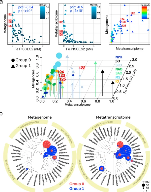
Given the clear patterns in the community responses to iron availability, we next wondered which molecular patterns were associated with them. Wefirst examined the prevalence of the diatom ISIP genes in more detail using both metagenomics and metatranscriptomics data to detect changes in gene abundance and expression, respectively. We found that both the abundance and expression of this gene family displayed a strong negative correlation with iron (Figure 5a). Figure 5a shows a strong hyperbolic profile of ISIP gene abundance and mRNA levels with respect to iron concentrations (nonlinear regressionfitness of 97.01 and 98.14, respectively; Table S1c). Furthermore, density clustering algorithms detected two types of responses—stations in which ISIP was only increased in metagenomics data (denoted group 0) and others in which both metagenomic and metatranscriptomic data showed increases in ISIP levels (denoted group 1; Figure 5a). The former likely correspond to locales where ISIP copy numbers vary in diatom genomes as a function of iron, implying that the diatoms at these stations display permanent genetic adaptations to the ambient iron concentrations, whereas the latter display transcriptional variation, indicative of moreflexible short‐term acclimatory rather than permanent adaptive evolutionary processes. Taxonomic analyses revealed that diatoms from the Thalassiosira genus were typical of group 0, whereas Pseudo‐nitzschia was found largely in Group 1 (Figure 5b). Representatives from both these genera are well known to respond tofluctuations in iron (Cohen et al., 2017; see supporting information S1 ‐ Claustre et al., 2008), so these different iron‐response strategies may underlie why they are present in different IAAs; Thalassiosira is present in the Black and Turquoise IAAs whereas Pseudo‐nitzschia is only present in the DarkRed module, where it is negatively correlated to iron (Figure 2a; Table S1d).
It is interesting to note that sampling sites can be grouped in a similar way according to either their picocya-nobacterial community or diatom ISIP patterns in relation to iron levels (Figure 6). HLIV and HLIII codo-minate the Prochlorococcus community in group 1 stations, and these sites are also characterized by the presence of LLI, as well as the Synechococcus clades CRD1 and EnvB. Based on picocyanobacteria commu-nity composition, these stations tend to cluster together in a group of low‐iron stations from Indian and Pacific Oceans (TARA_52, 100, 102, 110, 111, 122, 124, 125, 128, and 137). On the contrary, group 0 ISIP stations were dominated by either Prochlorococcus HLI or HLII and by Synechococcus clades II or III. Among these stations, those from the high‐iron Mediterranean Sea (TARA_7, 9, 18, 23, 25, and 30) clustered together based on picocyanobacteria community composition (Figure 6).
Figure 5. Abundance and expression of diatom ISIP genes with respect to iron concentration estimates. (a) 2‐D scatter plots correspond to the correlation between gene abundance and iron (left), gene expression and iron (middle), and abundance and expression of ISIP genes (right). Pearson correlation coefficients (pcc) and p values are indicated in blue. Iron concentrations were estimated using PISCES2 model (Table S1a). In all cases, the abundance and expression of ISIP genes were normalized by the total diatom unigene abundance and expression, respectively, and were then scaled to the unit interval. The 3‐D plot shown below is derived from the three 2‐D scatter plots, with the color gradient representing the third dimension. The data were clustered using density clustering algorithms, resulting in a group of Tara Oceans sampling sites in which ISIP was only increased in metagenomics data (denoted Group 0 stations [40 stations; circles]) and others in which both metagenomic and metatranscriptomic data showed increases in ISIP levels (denoted group 1 stations; 21 stations; triangles). The values corresponding to Tara Oceans stations in the Marquesas archipelago are labeled (122–125). Tara Oceans sampling sites are colored according to the ocean region in the 3‐D plot: NPO = North Pacific Ocean; SO = Southern Ocean; SPO = South Pacific Ocean; NAO = North Atlantic Ocean; SAO = South Atlantic Ocean; MS = Mediterranean Sea; IO = Indian Ocean. (b) Relative abundance (left) and expression (right) of ISIP genes assigned at different levels of resolution in a diatom phylogenetic tree. The color code corresponds to the two clusters of stations defined in panel a based on ISIP patterns (red for group 0 with variations only at metagenome levels; blue for group 1 with variations in both metagenome and metatranscriptome levels).
Figure 6. Comparison of iron‐driven changes in diatom ISIP gene abundance and expression and in the picocyanobacterial community from surface waters. Histograms of cell abundance of Synechococcus and Prochlororococcus clades at each Tara Oceans station are displayed, with stations sorted by hierarchical clustering of a Bray‐Curtis distance matrix. The left panels indicate iron concentration estimates from PISCES2 model, and metagenome and metatranscriptome levels of diatom ISIP genes, including the resulting cluster type (circles and triangles as described in Figure 5).