A modeling of Thulium laser in glass

ISMRE2018/XXXX-2018 ALGERIA

A modeling of Thulium laser in glass

1

Equipe Optoélectronique, Laboratoire de Développement des Energies Nouvelles et Renouvelables en Zones Aride, Université de Ouargla, 30000 Ouargla, Algeria

Corresponding Author email address [email protected]

Abstract— The aim of this work is the modeling of a

thulium laser in glass. We proposed a simplified three-level model of thulium laser, and we solved numerically the temporal evolution of the population in function of puissance pump.We found that the threshold value is equal to 110mW. The results of this simplified model were acceptable within the approximations taken.

Keywords—modeling, thulium laser, doped glass, rare earth ions.

I. INTRODUCTION

The discovery of optical fibers and lasers led to a revolution in the world of communications, where researchers were able to doped glass fibers with some rare earth element ions (Tm+3, Er+3,…) to obtain high-gain amplifiers. These fibers were not only used in amplifiers but were also used to be used as an active media for the production of optical fiber lasers. Among these optical fiber lasers, Thulium-doped fiber amplifiers (TDFAs) have recently been developed and characterized for optical communications [1, 2]. Several studies have been conducted on this type of laser, which has the potential to operate on several wavelengths of pump. There are some theoretical modeling studies on the thulium doped glasses, such as silica glass fiber [3], tellurite glasses lasers [4] and ZBLAN optical fiber [5]. Based on these studies, we will propose a simplified model of a thulium laser system, and then we will solve numerically this system and discuss its results.

II. NUMERICAL MODELING OF THULIUM LASER

In order to study and interpret the population dynamics in the chosen laser system, we proposed a simplified theoretical model based on the analysis of the equations of the evolution of the population densities of the various energy levels. The proposed model does not take into account the energy transfers for simplification, and we consider that the change in the level population and energy levels occurs only within a very small section of the optical fiber.

A. Description of the studied system

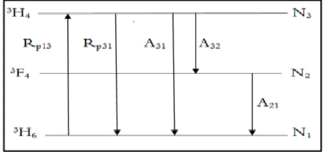
In theoretical processing we assume a three-level laser system that operates according to the pumping scheme shown in Fig.1. The pumping wavelength selected in this study is estimated at 790 nm, which pumps the atoms by 𝑅P13 Of the level (3H6 ) → (3H4) While they are come down

by RP31 Of the level (3H4)→ (3H6 ) . The atoms come down

quickly from the level (3H4 ) → (3F4 ) By 𝐴32, As well as

from the level (3H4)→ (3H6) By 𝐴31. These atoms are hunted

at the level (3F4 ) Which has a long lifetime that allows to

dictate (reconstruction) this level, while this level emptied by

𝐴2 to the bottom level (3H6 ). Laser emission occurs at 2µm

corresponding to the transition (3F4 ) →(3H6 ).

Fig. 1. Schematic of three-level laser.

Rate equations are given in this case as follows:

𝑑𝑁1 dt = RP31N3− RP13N1 + A21N32+ A31N3 (1) 𝑑𝑁2 dt = A31N3− A21N32 (2) 𝑑𝑁3 dt = RP13N1− RP31N3 − A21N32 (3) Where: 𝑅P13= σ13 Ip

hʋ_p: Pumping rate from level 3

H6 to level 3H4.

RP31 = σ31 Ip

hʋp: Pumping rate from level 3

H6 to level 3H4.

𝜏2: The spontaneous lifetime of 3F4 level.

A31: The spontaneous transition rate between the energy

levels 3H4 and 3H6.

A32: The spontaneous transition rate between the energy

levels 3H4 and 3F4.

A21: The spontaneous transition rate between the energy

levels 3F4 and 3

H6.

III. RESULTS AND DISCUSSION

A. Numerical solution of rate equations

We solved the differential equations (the rate equations) by the Matlab program (MATLAB) which contains a set of specialized functions to solve such equations, known as “ode” such as: ode45, ode23, ode15s, ode23s and ode23t. These functions differ from each to other in the degree of accuracy and effort required of the computer when used, and in the type of problem to be studied. Depending on the type of problem, the accuracy of the function and the speed of its

operation vary, so prefer to choose the right type to solve the problem appropriate

The study of the proposed system leads to the study of a two energy level system, based on the assumption that the third-level population turns to zero, ie pumping directly to the second level. Laser vibration occurs between 3F4 and 3H6

levels, under 790 nm excitation [5], the Tm+3 ions are excited from the 3H6 ground level to the 3H4 excited level, because

the lifetime of this level (3H4) is very small, these ions pass

almost simultaneously to the lower level 3F4 (Here is the

laser upper level ) whose lifetime is relatively large (within 10ms) Leading to the start of its population, while the ground level 3H6 (here is the lower level of laser) is emptied. Since

the lifetime of the latter is infinite (ground level), atoms of

3

F4 level descend spontaneously towards the ground level. In

order to obtain the effect of the laser, the condition of the inversion of population must be achieved, ie, the second-level populations greater than these of the first second-level of the laser. For this, the pumping rate must be considered sufficiently.

Table 1 shows the parameter values used in our Matlab program.

TABLE 1: NUMERICAL PARAMETER USED IN THE SIMULATION.

B. Determination of threshold power for laser effect

As mentioned in the previous section, in order for the laser effect to occur, the condition of the inversion of population, which depends on the amount of pumping rate, must be achieved. There is a threshold pumping rate corresponding to the threshold pump power, after which the laser begins to work.

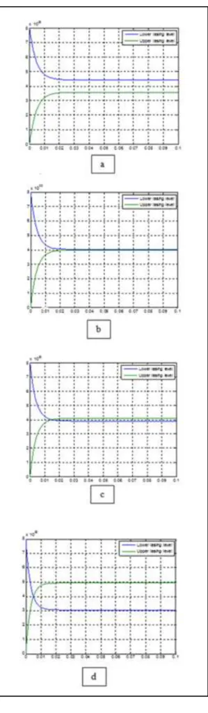
To determine the threshold power value in our proposed model, we simulated the time evolution of the population densities for different values of pumping ratios. Fig. 2 shows the variation in the population densities in terms of time for different values of pumping rates.

Fig.2. Population densities variation in terms of time for power values: (a) 90mW, (b) 110mW, (c) 120mW, (d) 180mW Ref Unit Value Parameter [4] m 7.9×10-7 𝜆𝑝 [5] s-1 75.1 𝐴3 [5] s-1 123.8 𝐴2 [6] m2 2.8×10-25 σ13 [6] m2 1.274×10-24 σ31

It is possible to observe from the general shape of all curves that they are characterized by two areas: The first is an area of increasing or decreasing of population, which corresponding of the process of population or depopulation of levels under the influence of pumping. The second area is a stabilization zone (of saturation) and is consistent with the steady state ( 𝑑𝑁_𝑑𝑡𝑖= 0), where the population densities of the two levels have a constant values under continuous pumping effect.

We also note that the power limit value to obtain the effect of the laser effect (inversion of population)is within 110mW Figure 2(b), at this value, the two population densities to the two levels are equal in the steady system (𝑁1= 𝑁2≈𝑁₂𝑇). Pumping must therefore be selected so that

the pump power is greater than this Limit value. if the pump power is less, the ground level population is always higher than the upper level rate and there is no population inversion As shown in Fig.2(a). When pumping is equal to the threshold power, the difference of population is zero and there is no amplification. At the higher values than the threshold power value, the second level population of the laser is greater than the first level population in the steady state and the difference of population is positive as shown in Fig. 2(c) and Fig.2(d).

C. Temporal variation of the the difference of population

Fig. 3 shows the temporal variation of the difference of population between the laser levels considered in in function of pumping power. We can observe the effect of pumping on the population inversion: the higher the pumping capacity, the greater the value of the difference population, ie the increase in the second level population and the decrease in the first level population.

Fig.3. Temporal variation of the difference of population.

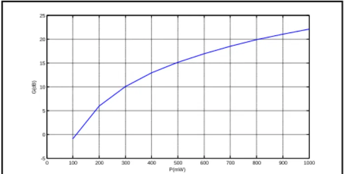
D. Gain variation

Fig. 4 shows gain variation in terms of pump power. We can note that the higher the pumping power, the higher the laser gain value, where the gain is greater than 20dB within limits 1000mW.

Fig.4. Variation of gain in function of pump power.

IV. CONCLUSION

After proposing a theoretical model to study a thulium laser of three-level system based on the analysis of the equations of the development of the population densities of different energy levels, and based on a Matlab program, we found the following results: variation of the population densities in terms of time for several values of power, time variation of the difference of the population as a function of pumping power and gain changes in terms of pump power. After analyzing and discussing these results, we determined that for the laser to occur, the condition of the inversion of population must be achieved, which can only be reached if the pumping power is greater than the threshold value set at 110 mW. As we have seen, the higher the pumping power, the greater the value of the difference in population. Gain is also increasing with increasing pump power and can be within 20dB within limits 1000mW.

REFERENCES

[1] Khamis M, Ennser K. Model for a Thulium-Doped Silica Fiber Amplifier Pumped at 1558 nm and 793 nm. International Journal of Engineering and Advanced Technology 2016; 5(4):76-80.

[2] Emami, S. D, Harun S. W, Abd-Rahman F, et al. Optimization of the 1050nm pump power and fiber length in single-pass and double-pass thulium doped fiber amplifier. Progress In Electromagnetics Research B 2009; 14:431-448.

[3] Jackson S. D, King T. A. Theoretical modeling of Tm-doped silica fiber lasers. Journal of Lightwave Technology 1999;17(5), 948-956. [4] Taher M, Gebavi H, Taccheo S, et al. Novel calculation for

cross-relaxation energy transfer parameter applied on thulium highly-doped tellurite glasses. In: Proc. SPIE 8257, Optical Components and Materials IX, 825707-6 (1 March 2012)

[5] Tessarin S, Lynch M, Donegan JF, Maze G. Thulium doped ZBLAN fibre ring-cavity amplifier. Proc. SPIE 5825, Opto-Ireland 2005: Optoelectronics, Photonic Devices, and Optical Networks, (3 June 2005)

[6] Keiser G. optical Fiber Communication, 3nd edn. Mcgraw – Hill Internationl editions Series in Electrical Engineering, 2000; P. 19-21.

0 100 200 300 400 500 600 700 800 900 1000 -5 0 5 10 15 20 25 P(mW) G (d B )