Object Predetection Based on Kernel Parametric Distribution Fitting
Jean-Philippe Tarel
LCPC, DESE
58 Bd Lefebvre, 75015 Paris, France
Jean-Philippe.Tarel@lcpc.fr
Sabri Boughorbel
Philips Research WB-4.63
5656 AE Eindhoven, The Netherlands
Sabri.Boughorbel@philips.com
Abstract
Multimodal distribution fitting is an important task in pattern recognition. For instance, the predetection which is the preliminary stage that limits image areas to be pro-cessed in the detection stage amounts to the modeling of a multimodal distribution. Different techniques are avail-able for such modeling. We propose a pros and cons analy-sis of multimodal distribution fitting techniques convenient for object predetection in images. This analysis leads us to propose efficient and accurate variants over the previously proposed techniques as shown by our experiments. These variants are based on parametric distribution fitting in the RKHS space induced by a positive definite kernel.
1. Introduction
The detection of complex objects still is a difficult task due to the intrinsic complexity of the objects to be detected, and also due to the variability of objects’ appearances. This usually leads to computationally intensive detection algo-rithms. To speed up the detection process, two kinds of ap-proaches are usually followed: the coarse to fine approach or the predetection approach. In the coarse to fine approach, different levels of degraded object models are used within the same detection algorithm to focus only on interesting areas of the image, see for instance [6, 8]. The second ap-proach consists in designing an alternative algorithm named predetection which is faster and usually based on the detec-tion of simple partial features associated with the object. A simple example of such a partial feature is image patch. Hence, the predetection allows, for detection algorithm, to focus only on interesting areas.
The predetection consists in scanning the image to de-cide which patches correspond to the object to be detected. In [5], SVM clustering was used to solve such problem. As underlined in [5], such approach gives good results at the price of a careful and relatively painful selection of the neg-ative examples. In this paper, we are interested in the
detection using only positive examples. Therefore, the pre-detection problem is not set as a clustering problem but as the modelling of a multimodal distribution (md) of the ob-ject patches over the space of possible image patches. One may think to use different md fitting techniques to achieve this modeling. The key problem is that most of theses md fitting techniques were designed and applied on spaces with a relatively small number of dimensions or have a complex-ity related to the number of positive samples. Whereas, in practice, to be informative enough, an image patch has eas-ily more than 20 dimensions and the number of positive ex-amples is large. We are thus trying to answer the question: within the already proposed md fitting techniques, which ones is able to tackle spaces of large dimensions with nu-merous samples?
In this paper, we focus on multimodal distribution fitting techniques based on kernel parametric distribution fitting in the RKHS space induced by a positive definite kernel. In section 2, we detail the predetection process. In sections 3, 4 and 5, we review different algorithms for multimodal distri-bution fitting and we discuss advantages and disadvantages with respect to the predetection task. Several new variants convenient for the predetection problem are proposed. At last, in section 6, results on experimental comparisons of the different algorithms and variants are described and dis-cussed.
2. Object Predetection
Road transportation applications raise increasing a num-ber of detection problems, such as lane-markings detection or sign detection. For sign detection, color is the obvious feature that is used to perform the predetection. However, this choice of feature is relatively specific to signs. A more generic choice of feature consists in small image patches. In practice we used image patches of 7 × 7 pixels size. Each patch is simply represented by a vector of 7 × 7 × 3 = 147 components containing the RGB values of the concatenated pixels.
(a) (b)
(c) (d)
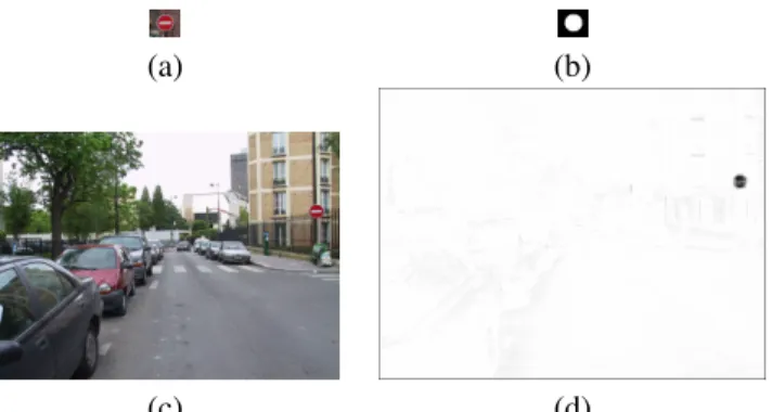
Figure 1. (a) is the sign used for learning 7x7 image patches on the object to be detected. (b) is the associated mask. (c) is an origi-nal image. (d) is the associated predetection map where possible sign patches are shown in dark.
in small overlapping image patches each one being repre-sented by a patch vector. An example of object of interest is the sign shown in Fig. 1(a)(b), which is used to learn the dis-tribution of patch vectors. After modeling this multimodal probability distribution with one of the techniques described in the following sections, it is easy to perform predetection by scanning patches of any new image. For instance, pre-detection of the sign learned only from Fig. 1(a), was per-formed on the image of Fig. 1(c). The obtained result is shown in Fig. 1(d), where dark values correspond to possi-ble location of the sign. Notice that despite a poor learn-ing database, the predetection is satisfylearn-ing enough. Patches having a probability higher than a threshold are considered to be from the object. This threshold can be, for instance, set to the min value of the probability over positive exam-ples.
3. Parzen Pdf Fitting
One of the most classical way for estimating a pdf from samples is the so-called Parzen windows technique:
p(x) = 1 m
i=mX
i=1
fσ(kxi− xk) (1)
where f is a positive decreasing function on R+. Most of
the time, f is taken as the normal distribution: fσ(t) =
1 (√2πσ)de
−t2
2σ2 (2)
When Parzen technique is applied on a space of large di-mension, i.e when d is large, numerical problems appear in (2) due to its denominator. Indeed, for σ > 1, the value
of f is very small for most of the t, since the term σdin
de-nominator is very large. To bypass this numerical problem, we get rid of the denominator which is common to all terms in (1). The fact that the obtained p function is not a pdf anymore is not a problem since the predetection threshold is rescaled accordingly.
The advantage of using the Parzen technique is that the learning stage consists only in selecting the parameter σ and the predetection threshold, by cross-validation, for example. Given a new patch vector x, the complexity for computing its probability to be within the object of interest is O(md). This is relatively computationally intensive when the num-ber m of samples is large.
4. Adaptive Pdf Fitting
In (1), only one parameter σ has to be set. In statistics, there exists a large literature on adaptive pdf fitting algo-rithms, see [2, 7] for instance, where the pdf is assumed to have many unknown parameters. For example, the scale σi
associated to each xiis assumed to be unknown. The pdf
model is in such case given by: p(x) = 1
m
i=mX
i=1
fσi(kxi− xk) (3)
To estimate these parameters, iterative algorithms were proposed. Two interesting algorithms may be recalled, the Abramson law [7], and the algorithms derived using a max-imum likelihood approach [2].
The numerical problem due to normalization which was underlined in the previous section for Parzen technique leads the adaptive pdf fitting algorithms to fail numerically for spaces of large dimensions. Indeed, the denominators in (3) are all with very different orders of magnitude.
5. Kernel Parametric Distribution Fitting
Statistical learning, particularly kernel methods, are more and more used in the pattern recognition field where the choice of priors is usually required. We now review the approach proposed by [4, 3], we named Kernel Paramet-ric Distribution Fitting which applies nicely to predetection. We also extend this approach by taking care of possible nu-merical instabilities. Compared to the Parzen technique, the training stage of the kernel approach is more computation-ally intensive, however, the complexity for evaluating the interest of a given patch can be drastically reduced and be-comes not directly related to the number of learning exam-ples as explained in Sec. 5.2.
5.1. Feature Subspace
Rather than performing a parametric distribution fitting in the original vector space, the fitting is performed in the RKHS space obtained by the mapping ϕ induced by the choice of a positive definite kernel k. Usually, ϕ(xi), where
xi, 1 ≤ i ≤ m are the m patch vectors, spans a subspace of
reduced dimension, where the parametric distribution only needs to be fitted. To obtain such subspace a Kernel PCA, without centering, can be performed. The centering is not necessary to find the linear subspace spanning ϕ(xi). The
process thus consists in an eigen decomposition of the Gram matrix Γ = (k(xi, xj)), 1 ≤ i, j, ≤ m. Then, only
eigen-values larger than a threshold η are kept. Finally a matrix M can be build allowing the projection of any vector from the original space in an orthonormal basis of the feature sub-space spanned by the ϕ(xi). The projection matrix is given
by M = D−1
2Rt, where D is a diagonal q × q matrix with
the q largest eigenvalues, and R is the m × q matrix of the associated eigenvectors.
Gram-Schmidt orthonormalization was originally used by [3] to compute M. This choice lacks for two reasons. The procedure is not invariant to patch vector permuta-tions xi. More annoying, Gram-Schmidt
orthonormaliza-tion presents also some numerical instability. On the con-trary, eigen decomposition leads to stable computations, and M is invariant to vectors arrangement.
A classical choice for kernel k is the Gaussian kernel k(x, x0) = e−kx−x0 k2
2σ2 , but other positive definite kernel can
be used such as the Laplacian kernel k(x, x0) = e−kx−x0 kσ ,
the Cauchy kernel k(x, x0) = (1 +kx−x0k2
σ2 )−1. The
opti-mal choice of the kernel is related to the investigated appli-cation, like in SVM learning.
5.2. Gaussian Fitting
Given any vector x of the original space, its coordinates in the orthonormal basis of the feature subspace are MX, where M is the q×m matrix previously computed and X = (k(xi, x)), 1 ≤ i ≤ m. The multimodal distribution fitting
is simply performed by a parametric fitting in the feature subspace previously defined.
We choose the normal distribution as the parametric model. The main advantage is the simple way for estimat-ing the normal distribution parameters, i.e, this estimation is closed-form. For instance, when the mean A of the dis-tribution is assumed unknown, it is estimated by averaging, in the feature subspace, the projections of m vectors: A =
1 m
Pm
i=1M Gi, where Giis the column i of G. The full
co-variance matrices C can also be assumed unknown as pro-posed in [3], and then estimated using empirical covariance matrix expression: C = 1 m Pm i=1(M Gi− A)(MGi− A)t. −5 0 5 10 0 0.5 1 1.5 x density data points true pdf mean diag cov mean full cov diag cov full cov
Figure 2. Same data set is fitted with different Kernel Gaussian distribution models.
Unknown mean and unknown full covariance matrix leads to q + 1
2q× (q + 1) unknown parameters which may
seem a relatively large number. We thus investigate model fitting with a reduced number of parameters such as un-known diagonal covariance matrix and isotropic covariance matrix with an unknown scale. For each of these last two cases, closed-form solution exists. In Fig. 2, we compare fitted pdfs obtained on the same 1D datasets, with known zero mean and unknown diagonal or full covariance matrix, and with unknown mean and unknown diagonal and full co-variance matrix. In experiments, we obtained that the use of isotropic covariance matrix is too restrictive in practice.
Gaussian distribution model leads to easy parameter esti-mations. With other models, such as Laplace model, closed-form solutions are not available. Nevertheless, iterative esti-mators derived in the context of M-estiesti-mators may be used. Notice that the resulting distribution is not normalized to one over the original space. Again, for predetection, the fact that the obtained model is not a probability function is not a problem. With the previous algorithm, given a new patch vector x, the complexity for computing whether this patch belongs to the object of interest or not is O(mdq), where q is the number of eigenvalues larger than threshold η. The complexity is thus higher than that of the Parzen approach. However, Incomplete Cholesky Decomposition using sym-metric pivoting (ICD) [1] of the gram matrix Γ = LtL
can be used with advantages before performing the eigen decomposition. Indeed, ICD allows to select a subset of q vectors ϕ(xi) which spans completely the feature
sub-space. The selection is no more performed after the eigen decomposition but before by removing vectors associated to a diagonal term on L lower than η. As a consequence, the complexity for testing a new patch becomes O(qdq). The complexity does not depends anymore on the size of the training data set. This is a very important property for real applications.
6. Experiments
Algo Uniform Gauss Cauchy
Parzen σ =.5 1.28±0.01 0.36±0.08 0.73±0.04 Parzen σ =1 0.79±0.08 0.33±0.10 0.52±0.07 Abramson 0.69±0.09 0.42±0.12 0.58±0.13
ML 0.79±0.23 0.63±0.30 0.52±0.16
mean diag cov 0.78±0.09 0.70±0.15 0.59±0.12 mean full cov 0.38±0.09 0.69±0.14 0.61±0.12 diag cov 0.45±0.05 0.47±0.10 0.60±0.13 full cov 0.37±0.09 0.69±0.14 0.61±0.12
Table 1. Average area error comparison for different types of noise distributions (bi-modal uniform, bi(bi-modal Gaussian, bi(bi-modal Cauchy) versus the algorithm type, on 1000 random realizations.
To evaluate the performances of the various previously described multimodal distribution fitting techniques, we run synthetic experiments with known true random 1D distribu-tions. Experiments with larger dimensions would have been very time consuming. Depending on the shape of the true distribution, we notice that the results may change. There-fore, we did experiments with a bimodal Gaussian distribu-tion, a bimodal uniform distribudistribu-tion, and a bimodal Cauchy distribution. For each distribution type, we generate 1000 realizations of 20 samples, 10 samples for each mode. A relatively small number of samples is used to simulate the usual sparsity of random samples obtained in spaces of large dimensions. In Tab. 1, the average area errors between the true distributions and the fits are shown. Seven multimodal distribution fitting techniques are compared. The two first lines are for Parzen with different values of the scale σ. The correct value of σ is one, notice how much a different value decreases the accuracy of the estimation. The next two lines presents the results for two adaptive techniques: the Abram-son law and the maximum likelihood approach. These two techniques do not apply well for spaces of large dimensions, however it is interesting to see that, in 1D, they do not de-crease the average errors for the Cauchy case, they are bet-ter for the uniform case, and are worst for the Gauss case compared to Parzen. The last four lines present results with Kernel Gaussian distribution fitting assuming different kind of unknown parameters: mean and diagonal covariance ma-trix, mean and full covariance mama-trix, diagonal covariance matrix, and full covariance matrix. The kernel k used is the Cauchy kernel with fixed same scale σ = 8 and we set η= 10−5. From this table, it appears that results are always
better when the mean is assumed known compared to when it is assumed unknown. Results with the full and diagonal
covariance matrix are often different. However, ranks are highly related to the shape of the true distribution.
It is worth noting that Kernel Gaussian fitting techniques achieve comparable or better performances for the uniform case compared to Parzen technique with the true scale. In the Gauss and Cauchy case, average errors for the Kernel Gaussian fitting techniques are a little higher, but it may be due to the fact that the kernel scale was tune for the uniform case.
7. Conclusions
We have formalized the predetection of complex object from image patches as a multimodal distribution fitting and we have shown that Kernel Gaussian fitting is an efficient solution in term of complexity during the scanning of a new image. Kernel Gaussian fitting is better in term of com-plexity compared to Parzen approach, thanks to the use of the incomplete Cholesky decomposition. The complexity does not depend anymore on the size of the training data set. Moreover, our experiments suggest that Kernel Gaus-sian fitting may be also more accurate in estimating the true distribution. Kernel Parametric distribution fitting can be used with other models than the Gaussian model leading to eventually more robust distribution fitting algorithms. We believe that such kind of algorithm may find valuable appli-cations outside predetection.
References
[1] S. Fine and K. Scheinberg. Efficient SVM training using low-rank kernel representations. Journal of machine Learning Re-search, 2, 2001.
[2] M. Jones and D. Henderson. Maximum likelihood kernel den-sity estimation. Technical report, Univerden-sity of Newcastle, 2004.
[3] R. Kondor and T. Jebara. A kernel between sets of vectors. In Proceedings of the ICML, 2003.
[4] S. Mika, B. Sch¨olkopf, A. J. Smola, K.-R. M¨uller, M. Scholz, and G. R¨atsch. Kernel PCA and de–noising in feature spaces. In M. S. Kearns, S. A. Solla, and D. A. Cohn, editors, Ad-vances in Neural Information Processing Systems 11. MIT Press, 1999.
[5] E. Osuna, R. Freund, and F. Girosi. Training support vector machines: an application to face detection. In Proceedings of the IEEE Conference on Computer Vision and Pattern Recog-nition, Puerto Rico, 1997.
[6] H. Sahbi, D. Geman, and N. Boujemaa. Face detection using coarse-to-fine support vector classifiers. In Proceedings of the IEEE International Conference on Image Processing, pages 925–928, 2002.
[7] P. Van Kerm. Adaptive kernel density estimation. Stata Jour-nal, StataCorp LP, 3(2):148–156, 2003.
[8] P. Viola and M. Jones. Robust real-time object detection. International Journal of Computer Vision, 57(2):137–154, 2004.