CFD Assessment of Car Park Ventilation System in Case of Fire Event

(1)

Faculty of Mechanical Engineering

A Thesis presented to the School of Engineering of Sapienza University of Rome in Partial Fulfillment of the requirements for the degree of

MASTER OF SCIENCE

Candidate: Ramin Rahif Matricola 1772459

Supervisors:

Prof. Alessandro Corsini Dr. Giovani Delibra

(2)

Acknowledgments

It is always a pleasure to remind the excellent people in the Sapienza university of Rome for their sincere guidance and help I received to fulfill my requirements to improve my experimental and theoretical skills and finally get my Master of science degree.

First, I would like to thank my supervisor Prof. Alessandro Corsini, for his belief and trust in me to accept me as a thesis student. He has always constructive comments, directions and continuous support and help.

Secondly, I would like to express my deepest thanks to Dr. Giovani Delibra who despite being extraordinarily busy with his duties, took time out to hear, guide and keep me in the correct path and helping me to carry out my project.

I would like also to thank my dear family for their full supports, prayers, encouragements and blessings as always.

Finally, I express my deepest gratitude to Sapienza university of Rome which provided everything required during my studies and made me feel like home.

Sincerely, Ramin Rahif Rome June 2019

(3)

ii

Abstract

Air quality in buildings is one of the most important factors for the occupants’ health and comfort. Designing heating, ventilation and air conditioning systems (HVAC) to achieve an acceptable air quality is one of the challenges during a building construction. In most cases including car parks, in addition to retain the air quality in normal condition, the existing ventilation system should act properly in case of fire event. As an emergency situation may lead to an incalculable life damage for the people inside the car park, the proposed ventilation system must be modeled and analyzed using computational fluid dynamics (CFD). The CFD will predict the airflow behavior allowing the assessment of the ventilation system effectiveness.

One of the most efficient and recent ventilation systems used in car parks is based on utilizing impulse fans which are commercially known as jet fans. Jet fans have pumping effects which force the air movement from supply to the extraction points. So, the positioning of the system components within the car park plays a significant role in the efficiency of the impulse ventilation system (IVS). The best strategy is to avoid the airflow deviations by placing the extraction and supply points on the opposite walls. It can be conducted easily in simple and small geometries, but for the real cases such as a huge and complex car park, implementing the mentioned technique is questionable. In this study, the applied ventilation system of a commercial building car park was analyzed to derive the interaction between the ceiling jet fans. The existing design had so many defects which are mostly related to the positioning of the jet fans. A sensitivity analysis was carried out considering the locations of the fire source and the velocity of the jet fans. OpenFOAM v1806 is used to run the CFD simulations. Finally, by examining the velocity and visibility distribution alongside streamline patterns in different fan positionings, the most efficient design in terms of smoke extraction is resulted.

(4)

iii

1 Introduction

Computational Fluid Dynamics is a numerical approach to predict the fluid flow characteristics in terms of velocity, temperature, pressure and heat transfer. It is also possible to extend the previous predictions to forecast visibility which can be restricted by smoke, produced by the fire. Recently, it is necessary to study the large-scale underground car parks to determine air quality which can be altered by vehicle pollutants entering the enclosed area. Also, it must predict smoke and heat propagation in case of fire. The latter is so important because a poor design of ventilation system may lead to incalculable life damage to the occupants.

The ventilation of underground car park is so important because inhalation of combustion products released by cars, especially CO will make health problems. Recently, a new mechanical ventilation system has appeared which they are based on jet fans mounted beneath the ceiling of car parks. These jet fans are able to confine contaminated air and restrict its dispersion. It should be considered that the exhaust flow-rate from car park should not be lower than the flow-rate induced by jet fans toward them. If the jet fan flow-rate is significantly smaller than the exhaust flow-rate, recirculating flows are generated and disperse pollutants. Before the use of jet fans for the ventilation of underground car parks ductwork system was the most common choice. These systems are so expensive due to the cost of necessary equipment, the large space occupied by ductwork and the huge head losses [1].

For an underground car park, the ventilation rate must be calculated to determine CO concentrations to have some pre-defined minimum levels. To do so, some requirements must be satisfied as: a) an average concentration of not more than 30 parts per million over an eight-hour period b) peak concentrations such as ramps and exits, of not more than 90 parts per million for periods not exceeding 15 minutes. Considering mechanical ventilation for an underground car park, the ventilation system must be capable of air change of 6 times per hour. For exits and ramps which vehicles may stop with engines running the same provision must be considered for 10 air changes per hour [2].

(7)

3

Impulse ventilation system (IVS) is mostly used for two purposes. Beside the capability of the IVS system to dilute the contaminated air caused by cars exhausts in normal condition it must be also capable of smoke dilution by providing the necessary ventilation in case of fire. Fire events are so hazardous as the smoke can disperse almost without any restrictions. Also, the smoke-free lower layer is diminished because of the low height at such car parks. As a result, the fire is hard to be located and extinguished by fire-fighters [3].

Unlike other buildings, car parks need some more parameters to be considered to confine the fire spread in the building. Two most important factors are: a) fire load definition b) if the story is well ventilated, the probability of the fire spread to the other floors is so low. The mechanical ventilation system designed for fire control must be independent of other ventilation systems which has to be capable to change the air in whole car park area 10 times per hour in case of fire. Also, the system must be designed in two independent parts which each should be able to conduct 50% of total air change and also each part can work simultaneously or individually [4].

The analysis conducted by CFD shows that the positioning of the impulse ventilation system components plays an important role in the efficiency of the ventilation system. Settling the exhaust and supply shafts in the opposite boundaries increases the efficiency of the system which leads to the flow of massive fresh air through the whole car park [5].

The efficiency of impulse ventilation system relies on the number of jet fans; too low jet fan components reduces the ability of the system to move the air toward the desired locations. Also, too high quantity of jet fans causes severe smoke recirculation which decreases the efficiency [6]. The IVS system function is similar to positive pressure ventilation (PPV) and is developed from longitudinal ventilation system implemented in tunnels [7].

In most cases, the impulse ventilation system is used together with the sprinkler system. According to the researches, using only the sprinkler system makes the smoke back layer too long which activates so many sprinklers. It makes problems for the firefighters to fight with the fire. Also, due to the pressure drop, the sprinkler system may not work properly. Utilizing two systems together has better results [8].

(8)

4

Some important factors must be taken into account when using both IVS and sprinkler systems alongside. The fire detectors which is responsible to activate the jet fans must have some delays in comparison to the detectors activating the sprinklers. If both detectors operate simultaneously, the IVS system delays the activation of the sprinkler system by moving plume of heat downstream and replacing it with cool air [9].

Comparing different types of ventilation system shows that the impulse ventilation system has better efficiency. It mostly relies on the architecture and geometry of the car park. In some cases, like an underground car park with many partition walls, it may not be logical to use IVS. In this case, almost half of the air inside the enclosed area has not sufficient extraction velocity [10].

As Computational fluid dynamics contains complex equations which have to be solved, it is necessary to use some tools to see the flow fields. Otherwise, it is difficult to obtain results and visualize them [11].

CFD simulations are used to predict the airflow behavior inside a car park. Then all the modifications and improvements are done regarding the jet fan positioning and choice. As dimensions are high in a common car park, this procedure may become time-consuming. Finally, it has to be determined if an IVS system suitable for the existing plan or the traditional ductwork system. In this thesis work an existing jet fan system designed for a commercial building located in Tabriz, Iran was studied for optimization and improvements by suggesting the jet fan positioning. Different designs with corresponding analysis were carried out in order to obtain the best choice.

(9)

5

2 Background and Governing Equations

2.1 What is Computational Fluid Dynamics (CFD)

Computational fluid dynamics is a numerical simulation tool which plays a significant role in technology enablers nowadays. Initially, it was used in the aeronautics and aerospace industry which has developed to become an essential tool in wide range of other design-intensive industries. Recently other industries also became the heavy users of CFD. For example, in electronics, it is used to simulate and optimize the energy systems and heat transfer for the cooling of electronic devices. Also, in the building industry CFD is used in HVAC (heating, ventilating, and air conditioning), in fire and air quality simulations [12].

Computational fluid dynamics is a recent computer aid tool used in engineering. It is because of the complex equations which have to be solved. The principle of equations are Navier-Stokes equations, It is sufficient to simulate and model with enough accuracy the whole types of flows from turbulent to laminar, incompressible to compressible and also the multiphase flows [12].

Fluids are gases or liquids which do not maintain any particular shape. Unlike solids, these states of material cannot resist shear stress and imposing large stress do not change their shape permanently. Motion is caused by shear stress in the fluids. In studying fluid flow, it is most important that what happens in the macroscopic scale rather than microscopic. The fluids can be considered as continuum which means that it is possible to achieve their behavior at any point in the flow field. Fluids can be categorized under Newtonian and non-Newtonian. The first case has a linear relationship between shear stress and shear rate. The slope between shear stress and the corresponding shear rate shows molecular viscosity. The molecular viscosity shows the resistance of the fluid toward the deformation. In non-Newtonian fluids, the same relationship is non-linear [12].

Fluids can be characterized by Navier-Stokes equations. These equations are non-linear second order partial differential equations governed by independent variables [12].

(10)

6

2.2 Eulerian and Lagrangian Description of Conservation Laws

Conservation laws define that a certain physical measurable quantity remains the same in a region for an isolated system. Conservation laws cannot be proven mathematically but can be expressed using mathematical equations.

There are two approaches to deal with the fluid flow and relating transfer phenomena which are Lagrangian (Material Volume, MV) or Eulerian (control volume). In the Lagrangian approach (Fig. 2.1a) the fluid splits into packs and each pack is monitored as it moves through space and time. These packs are marked according to their initial center of mass position x0 at

some initial time t0, and the flow is defined by a function 𝑥(𝑡, 𝑥₀).

Differently, in the Eulerian approach (Fig. 2.1b) a particular location in the flow field must be marked and monitored as time goes on. In such a way, the flow parameters are functions of time 𝑡 and position 𝑥. The fluid flow velocity in the field can be expressed by 𝑣(𝑡, 𝑥). The two specifications are related to each other as the derivative of the position of a pack 𝑥₀ dependent on time results in velocity,

𝑣(𝑡, 𝑥(𝑥

₀

, 𝑡)) =

𝜕

𝜕𝑡

𝑥(𝑡, 𝑥

0

)

(2.1) According to the above description, the properties of a fluid in a field can be measured either on a fixed point which particles are crossing it (Eulerian) or by monitoring a pack of particles within the field (Lagrangian). The following study utilizes a Eulerian approach to measure the fluid particles crossing a specific point in the flow field [12].

(11)

7

Computational fluid dynamics (CFD) is based on three basic physical principles: conservation of mass, of momentum and of energy. The governing equations in CFD are based on these conservation principles.

2.2.1 Reynolds transport theorem

The conservation laws are applicable to the material volumes rather than fixed points or control volumes. In order to extend these laws according to the Eulerian approach, Eulerian equivalent of an integral taken over a moving material volume of fluid should be considered which is known as Reynolds transport theorem.

Consider B as any characteristics of the fluid like mass, momentum or internal energy. So, the 𝑏 = 𝑑𝐵/𝑑𝑚 shows the value of B in any small element of the flow field. The rapid total change of B in the material volume (MV) equals to the rapid total change of the B inside the control volume (V) adding the net flux of B in or out of the same control volume over its surface (S). The Reynolds transport theorem results in,

(

𝑑𝐵

𝑑𝑡

) =

𝑑

𝑑𝑡

(∫

𝑉_(𝑡)

𝑏𝜌𝑑𝑉

) + ∫

𝑆(𝑡)

𝑏𝜌 𝒗

𝒓

. 𝒏 𝑑𝑆

(2.2)

𝜌 = the density of the fluid

𝑛 = the outward normal to the control volume surface 𝒗 (𝑡, 𝑥) = the velocity of the fluid

𝑣𝑠 (𝑡, 𝑥) = the velocity of deforming control volume

𝑣_𝑟 (𝑡, 𝑥) = the relative velocity which the fluid enters/leaves the control volume 𝑣_𝑟 = 𝑣(𝑡, 𝑥) − 𝑣_𝑠(𝑡, 𝑥)

If the control volume considered to be fixed without any deformation, 𝑣_𝑠 = 0 so the right-hand side of (Eq. 2.2) can be resulted using Leibniz rule as,

𝑑

𝑑𝑡

∫ 𝑏𝜌𝑑𝑉

𝑉

= ∫

𝜕 𝜕𝑡

𝑉

(𝑏𝜌)𝑑𝑉

(2.3) Simplifying and applying divergence theorem to convert surface integral to a volume integral, (Eq. 2.2) becomes,

(

𝑑𝐵 𝑑𝑡

)

𝑀𝑉

= ∫ [

𝜕 𝜕𝑡 𝑉

(𝑏𝜌)𝑑𝑉 + ∫ 𝑏𝜌𝒗 . 𝒏 𝑑𝑆

𝑆 (2.4)

(12)

8

Using substantial derivative and expanding the second term in the bracket an alternative equation can be derived,

(

𝑑𝐵

𝑑𝑡

)

𝑀𝑉

= ∫ [

𝐷

𝐷𝑡

(𝜌𝑏) + 𝜌𝑏 ▽ . 𝒗] 𝑑𝑉

𝑉 (2.5)

The (Eq. 2.5) can be used to obtain the Eulerian form of the conservation laws in a settled location [12].

2.3 Conservation of Mass

Conservation of mass also known as continuity equation shows, in the lack of any source or sink in the region, the corresponding mass remains constant. Let’s consider a material volume (Fig. 2.2) of mass m, density ρ, and velocity 𝒗, considering Lagrangian coordinate system the conservation of mass can be formulated as,

(

𝑑𝑚

𝑑𝑡

)

𝑀𝑉

= 0

(2.6)

Figure 32.2 conservation of mass for a material volume of a fluid of mass m [12]

For B = m the value of b =1, and with respect to (Eq. 2.5) the mass conservation can be expressed in the Eulerian coordinate system as,

∫ [

_𝑉 𝐷𝜌_𝐷𝑡

+ 𝜌 ▽. 𝒗] 𝑑𝑉 = 0

(2.7) In order to validate the above equation for any control volume V, the integrand should be equal to zero, the resulting differential form of mass conservation is as,

𝐷𝜌

(13)

9

_𝑥𝑥

𝜏

_𝑥𝑦

𝜏

_𝑥𝑧

𝜏

_𝑦𝑥

𝜏

_𝑦𝑦

𝜏

_𝑦𝑧

(14)

10

Considering Newtonian fluid and ignoring the effect of volumetric viscosity, the shear stress shown in (Eq. 2.14) becomes,

𝜏

_𝑖𝑗

= 𝜇 (

𝜕𝑢𝑖 𝜕𝑥𝑗

+

𝜕𝑢_𝑗 𝜕𝑥𝑖

− 𝛿

𝑖𝑗

(

2 3

)

𝛿𝑢𝑘 𝛿𝑥𝑘

)

(2.15) Where 𝜇 is the dynamic viscosity, 𝛿_𝑖𝑗 is Kronecker delta, and the subscripts I, j and k refer to the linear dimensions of the x, y and z [13]. An example of forces acting on a control volume in 𝑥 direction is shown in (Fig. 2.3).

(15)

11

2.5 Conservation of Energy

The equation which implies the total energy conservation is shown as, 𝜕 𝜕𝑡

[𝜌 (𝑒 +

𝑈2 2

) + ▽ . [ 𝜌 (𝑒 +

𝑈2 2

) 𝑈

+ 𝜌𝑓 . 𝑈

⃗⃗

(2.16) Where 𝑈2 _{= 𝑢}2_{+ 𝑣}2_{+ 𝑤}2_{is the magnitude of the velocity vector,}_{𝑒 = 𝑐}

𝑣𝑇 is internal

energy, 𝑞̇ is the energy source, 𝑘 is the thermal diffusion coefficient and 𝑇 is temperature. To derive the equation for the conservation of internal energy it is possible to subtract the results of momentum equations with their corresponding velocity vector from the total energy equation. So, the equation for the conservation of internal energy becomes,

𝜕(𝜌𝑒) 𝜕𝑡

𝜕𝑢 𝜕𝑦

+

𝜕𝑣 𝜕𝑥

)

2

+

(

𝜕𝑢 𝜕𝑧

+

𝜕𝑤 𝜕𝑥

)

2

+ (

𝜕𝑣 𝜕𝑧

+

𝜕𝑤 𝜕𝑦

)

2

]

(2.17) Where 𝜆 = −2

3𝜇 and 𝜇 shows dynamic viscosity [13].

(Eq. 2.9) to (Eq. 2.17) is applicable to a closed volume in a system. As the mentioned equations are non-linear partial differential equations it is extremely hard to be solved. By discretizing n time and space (closed volume) it is possible to find a numerical solution. To achieve a logical and accurate solution, it is necessary to use some iterative numerical methods like Semi-Implicit-Method for Pressure-Linked Equations (SIMPLE) [13].

(16)

12

2.6 The Discretization Procedure

Distribution of values of a dependent variable such as 𝜑 in a domain needs a numerical solution of the partial differential equations as mentioned earlier. It needs settling some points called grid points in their corresponding discrete elements which are not overlapping. This procedure is called meshing. The points usually constructed in the centroids or at the vertices of the elements. It mostly depends on the method used for discretization. The aim is to find discrete values of 𝜑 instead of the continuous solution of the partial differential equations. The procedure to convert the governing equation to a group of algebraic equations with discrete values of 𝜑 is known as discretization process and there are particular methods to derive these kinds of conversions denoted as discretization processes. The algebraic equations are solved according to their neighboring elements to calculate the discrete values of 𝜑. These algebraic equations are achieved by conservation equations governing 𝜑. As the values for 𝜑 is calculated, the data should be processed to get any required information. [12]. An example of the process which is applied to the study of the heat transfer case is illustrated in (Fig. 2.4).

(17)

13

(18)

14

The discretization process consists of different steps as, I. Geometry and Physical Modeling

II. Domain Discretization III. Equation Discretization

IV. The solution of Discretized Equations

The necessary discretization method used for a given differential equation can be chosen by the designer. Here are some most common methods that are used for discretization,

• Formulation for Taylor-Series • Variational Formulation • Weighted Residuals

• Control-Volume Formulation

Here, the Control-Volume discretization method is a unique version for the Weighted Residuals method. In this method, the domain is divided into several control volumes that are not overlapping. Every grid point is surrounded by a single element. Each sections profile representing the 𝜑 are utilized to derive the necessary integrals. Finally, for a set of grid points, the discretized values for 𝜑 are achieved [15].

The crucial characteristic of the Control-Volume method is that the final solution shows that the integral conservation of fluid properties is validated precisely for any group of the control volumes. This feature is independent of the element size. It does not imply that the coarse elements will not result in precise integral conservation [15]. Discretization method has different steps which are shown in (Fig. 2.5) [12].

(19)

15

Figure 2.5 The Discretization Procedure [12]

Physical Phenomena

Physical Domain

Domain Modeling Physical Modeling

Set of governing equations defined on a computational domain Domain Discretization Equation Discretization System of Algebraic Equations Numerical Solutions Structured Grids (Cartesian, Non-Orthogonal) Block Structured grids Unstructured grids Chimera Grids Finite Difference Finite Volume Finite Element Boundary Element Solution Method Combinations of Multigrid Methods Iterative Solvers Coupled-Uncoupled

(20)

16

2.7 Solving the System of Algebraic Equations

The methods for solving linear systems of equations are categorized in direct and iterative techniques. As the fluid flow equations are extremely non-linear, by linearizing them the coefficients are derived which are commonly dependent on the solution. As an accurate solution at each iteration is not our goal, so the direct methods for solving them mostly are not used. The iterative methods have lower computational cost and lower memory, so are most desirable for applications. After discretization of a set of linear equations 𝐴𝜑 = 𝑏 which 𝜑 is the unknown property settled in the centroids of the elements, are desired values. In this equation, the matrix 𝐴 is produced by the linearization process which gives some coefficients of unknown mesh geometry. On the other hand, 𝑏 is constructed from all boundary conditions, constants, non-linearizable components and sources.

2.7.1 Linear solvers

The linear solver specifies the solver used for each discretized equation. It is different from applications solver like simpleFoam exists in OpenFOAM which defines the whole set of equations and algorithms used to solve the problem.

The first step to set solver in OpenFOAM is to define the linear solver for the simulation. OpenFOAM has different solver for which can be used for calculating the flow field properties[16]. Here are the types of linear solvers in OpenFOAM:

• PCG/PBiCGStab: Stabilized preconditioned (bi-)conjugate gradient, for both symmetric and asymmetric matrices

• PCG/PBiCG: preconditioned (bi-)conjugate gradient, with PCG for symmetric matrices, PBiCG for asymmetric matrices

• smoothSolver: solver that uses a smoother

• GAMG: generalized geometric-algebraic multi-grid • diagonal: a diagonal solver for explicit systems

(21)

17 2.7.2 Iterative methods

When the high amount of the matrix elements are zero, it is not appropriate to use direct methods. It happens when the equations remain non-linear after linearization or when the problems are dependent on time. The latter is exactly what happens in fluid problems.

The iterative methods are more desirable because a part of the iterative solution process consists of the solution of the linearized system. Two most important iterative methods are

• Jacobi Method • Gauss-Seidel Method

For all methods, the coefficient matrix can be written as,

𝐀 = 𝐃 + 𝐋 + 𝐔

(2.18) Where 𝐷, 𝐿 𝑎𝑛𝑑 𝑈 are diagonal, strictly lower and strictly upper matrices. The iterative methods to solve a linear system like 𝐀𝛗 = 𝐛 continues to find solutions of 𝜑(𝑛) till some predefined conditions are satisfied, then it converges to the exact solution of the 𝜑. For this method an initial condition 𝜑(0)_{must be defined as initial point and the iterative method}

computes 𝜑(𝑛)_{from already computed 𝜑}(𝑛−1)_[12].

2.7.2.1 Jacobi method

This method is known as the easiest iterative method to solve a set of linear equations, which is illustrated in (Fig. 2.6)

Figure 2.6 Jacobi Method illustration

A system of equations considered as 𝐀𝛗 = 𝐁, if the elements located in diagonal are not zero, so the first equation for 𝜑1 can be solved, then the second equation for 𝜑2 comes after and so

(22)

18

and will continue till a new value 𝜑_𝑁 is calculated. It shows just one iteration. Each iteration result is considered as a new guess for the next iteration and the process is repeated. It will continue until the results from two consecutive iterations fall below some value known as convergence criterion. The solution is reached when it happens. In the Jacobi method, some estimate is given by 𝜑(𝑛−1)_{and an update is calculated by the equation below,}

𝜑

_𝑗(𝑛)

=

1 𝑎_𝑖𝑖

(𝑏

𝑖

− ∑

𝑎

𝑖𝑗

𝜑

𝑗 (𝑛−1)

) 𝑖 = 1,2,3, … , 𝑁

Here the Gauss-Seidel method can be described schematically as from the matrix for formula in (Fig. 2.7).

(23)

19

Figure 2.7 Gauss-Seidel graphical representation [12]

2.7.3 Multigrid approach

If the amount of algebraic equations increases the rate of convergence in iterative methods decreases significantly. It happens in any size of the system which confines the iterative solvers. A solution to this problem is proposed which is resulted from the combination of the iterative and multigrid approaches [12].

The iterative methods are able to eliminate high-frequency errors. On the other hand, these methods cannot cancel low-frequency components. So, these methods are named smoothers in the multigrid approaches [17]. As shown in Fig. (2.8) high-frequency errors are sensed by the element easily while as the frequency decreases the error becomes soother and just an small portion of it lies within a cell. Refining the grid makes these problem worse resulting in decrease of the rate of the convergence [12].

(24)

20

Figure 2.8 different error modes in 1D grid

2.7.4 Preconditioning

The preconditioner matrices make the eigenvalues of the 𝐵 matrix clustered allowing to achieve the solution faster than the main system. The new system has better spectral properties and is equivalent to the previous system. The preconditioners are used because the coefficients of the 𝐵 matrix are unforeseen which affect the convergence of the iteration method. The preconditioner is a matrix which gives us the defined transformation which is called 𝐏. It can be described in the system as,

𝐏

−1

𝐀𝛗 = 𝐏

−1

𝐛

(2.24) The new system has the same solution of the original with much better spectral properties of 𝐏−1𝐀.

The folder for preconditioners in the OpenFOAM [12]:

• DICPreconditioner, DILUPreconditioner: diagonal incomplete Cholesky preconditioner for symmetric and asymmetric matrices

• diagonalPreconditioner

• FDICPreconditioner: fast mode of DICPreconditioner which the correlative of the preconditioned diagonal and upper coefficients are divided by the diagonal are calculated and stored. It is used for symmetric matrices

(25)

21 • noPreconditioner: without any preconditioner

• GAMGPreconditioner: geometric agglomerated algebraic multigrid preconditioner which uses multigrid cycles as preconditioners

2.8 Turbulence Modeling

Due to high inertial terms, the laminar flows can become unstable. The turbulence is made of eddies with different dimensions which can break down to smaller eddies and transfer their energy to the nearby eddy [12].

There are many turbulence models for indoor environments simulations, including Reynolds averaged Navier-Stokes (RANS) and Large Eddy Simulation (LES). RANS turbulence modeling can be categorized in eddy-viscosity and Reynolds-stress models [18]. As shown in (Fig. 2.9), LES resolves scales with a shorter length than the RANS models resulting in better results. Although, they need high power computers than the methods using RANS models [19].

(26)

22 2.8.1 RANS

RANS eddy-viscosity models can be categorized by the number of transport equations utilized:

• Zero-Equation Eddy-Viscosity Models • One Equation Eddy-Viscosity Models • Two-Equation Eddy-Viscosity Models • Multiple-Equation Eddy-Viscosity Models

Two most popular turbulence models used in enclosed environment air simulation are denoted as 𝑘 − 𝜀 and 𝑘 − 𝜔 which are related to the Two-Equation Eddy-viscosity Models [18].

𝑘 − 𝜀 is one of the most used and popular turbulence models proposed in 1993 by Launder and Spalding [20]. It is respectively robust and simple for indoor environment simulation. The model can be formulated as,

𝑣

_𝑡

= 𝐶

_𝜇𝑘

2

𝜀 (2.25) Where 𝑣_𝑡 is turbulent eddy viscosity, 𝑘 is turbulent kinetic energy, 𝜀 is dissipation rate of turbulence energy and 𝐶_𝜇 = 0.09 is an empirical constant. This model mostly developed for flows with high Reynolds. In order to use for low Reynolds like wall functions and near-wall flows, it is necessary to connect the outer-wall free stream and the near-wall flow [18].

𝑘 − 𝜔 turbulence models which are reformulated and revised Wilcox [21] is applicable to both boundary layers and free shear flows which is not sensitive to finite free stream boundary conditions on the properties of turbulence. It is an accurate approach to the mildly separated flows and uncomplicated geometries. The 𝑘 − 𝜔 model proposed by Wilcox [22] is similar to 𝑘 − 𝜀 models, which is based on Boussinesq approximation. To determine two large scales of turbulence the relating two transport equations must be solved. The specific turbulence dissipation 𝜔 can be written as,

𝜔 =

𝜀

(27)

23

This approach has some advantages over the previous one as a) it is much easier to integrate, so is more robust b) without requiring extra damping functions it can be integrated through sub-layer c) it is more appropriate for the flow which has weak pressure gradient [12].

2.8.2 LES

Mostly, the common method for determining turbulence flows is to use RANS, however, in some cases, the designers encounter a situation which the RANS is not adequate. In these cases, alternative methods like Large Eddy Simulation (LES) or Direct Numerical Simulation (DNS) can be utilized. In LES the equations which are dependent on time are filtered to eliminate very small time and length scales. These methods require finer mesh with running for small time steps, especially for wall confined flows. Also, the time steps must be high enough in order to account for the correlations for the velocity components which are fluctuating. LES method results in more details in flow structure and fluctuations of pressure and Lighthill stresses, which cannot be derived using RANS method [23].

2.9 Standard Solvers in OpenFOAM

OpenFOAM does not have a general solver which can be applied for all the applications. Instead, it contains a folder of solvers which is subdivided with respect to continuum mechanics. Each solver has a descriptive name. For the present study, two different solvers are coupled. Initially, the solver for incompressible flows are used to simulate the velocity field, then the basic solver is coupled to model smoke propagation. Here the existing solvers for incompressible flow are categorized [24]:

• adjointShapeOptimizationFoam: steady-state solver for incompressible, turbulent flow of non-Newtonian fluids with optimization of duct shape by applying “blockage” in regions causing pressure loss as estimated using adjoint formulation

• boundaryFoam: Steady-state solver for incompressible, 1D turbulent flow, typically to generate boundary layer conditions at an inlet

• icoFoam: Transient solver for incompressible, laminar flow of Newtonian fluids • nonNewtonianIcoFoam: Transient solver for incompressible, laminar flow of

non-Newtonian fluids

• pimpleFoam: Transient solver for incompressible, turbulent flow of Newtonian fluids on a moving mesh

(28)

24

• overPimpleDyMFoam: Transient solver for incompressible, flow of Newtonian fluids on a moving mesh using the PIMPLE (merged PISO-SIMPLE) algorithm • SRFPimpleFoam: Large time-step transient solver for incompressible, turbulent flow

in a single rotating frame

• pisoFoam: Transient solver for incompressible, turbulent flow, using the PISO algorithm

• shallowWaterFoam: Transient solver for inviscid shallow-water equations with rotation

• simpleFoam: Steady-state solver for incompressible flows with turbulence modeling • overSimpleFoam: Steady-state solver for incompressible flows with turbulence

modeling

• porousSimpleFoam: Steady-state solver for incompressible, turbulent flow with implicit or explicit porosity treatment and support for multiple reference frames (MRF)

• SRRFSimpleFoam: Steady-state solver for incompressible, turbulent flow of non-Newtonian fluids in a single rotating frame

Also, openFOAM contains some basic solvers as following [24] • laplacianFoam: Laplace equation solver for a scalar quantity

• overLaplacianDyMFoam: Laplace equation solver for a scalar quantity

• potentialFoam: Potential flow solver which solves for the velocity potential, to calculate the flux-field, from which the velocity field is obtained by reconstructing the flux

• overPotentialFoam: Potential flow solver which solves for the velocity potential, to calculate the flux-field, from which the velocity field is obtained by reconstructing flux

• scalarTransportFoam: Passive scalar transport equation

(29)

25

2.10 Induction Fans

Jet fans are also known as induction or impulse fans pull the air flow from supply to extraction zones. They act as a source of velocity where the airspeed is low, guaranteeing ventilation of all zones in daily ventilation. As the impulse fans are mounted in specific points, they occupy only less than 0.5% of the ceiling area. This increases the space for other technical installations and also visibility across the parking [25].

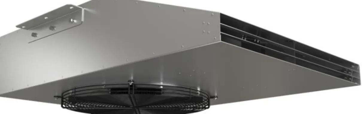
Induction fans are specially designed to be utilized in underground car parks. They are used for dual purposes, to provide normal ventilation and smoke extraction in case of fire. These fans are cost-effective in comparison to traditional ductwork system. Two most important advantages of the jet fans are a) reduction in installation cost (reduction in the cost of complex grilled and ducted system) b) running cost saving because of fan features [26]. Appropriate quantity of the jet fans must be chosen and distributed in the parking space to ensure the desired air movement. The control system can vary from simple timed to full pollution sense multi-stage system. When an emergency case initialized the main task of the jet fans is to move the air to the closest extraction point as shown in (Fig. 2.10 and 2.11). the smoke control system has to keep the escape roots clear and also makes a corridor for fire-fighters to deal with the fire source [27].

(30)

26

Figure 2.11 induction fan smoke extraction steps [26]

Induction fans work on tunnel ventilation principles, making jet with a high velocity which thrusts toward the air ahead of fan conveying momentum to surrounding air through entrainment. The volume of absorbed air is relatively larger than the air passing through the

1. Fire starts

2. Ventilation system starts to run

(31)

27

fan. Impulse fan performance is dependent on the thrust made by the fan which is the product of mass flow rate times velocity change. In other words, it is equal to volume flow times air density times fan outlet velocity which is measured in Newtons [28]. Impulse fans fall in two categories considering their shapes as shown in (Fig. 2.12).

Figure 2.12 (a) Jet Thrust Fan (b) Induction Thrust Fan

(32)

28

2.11 Axial Fans

Axial fans (Fig. 2.13) as their name implicate the direction of the flow through them is a kind of mechanical fan. These fans mostly are recognizable for the people as window fans or box fans. Both the direction and speed of the axial fan is controllable. They are used in many industrial, commercial and residential buildings with different sizes. Sizes of axial fans ranges from very small that a person can hold it in hand to very huge ones used in industrial facilities and huge buildings.

Axial fans have some advantages over other kinds of fans. One of the most important characteristics of axial fans is that they can move a large amount of air so quietly. Long lifespan, low price and optimum performance make them the most popular choice in many ventilation systems.

Figure 2.13 Axial Fan

Axial fans are used in buildings specifically in underground car parks to maintain the indoor air quality. These fans are vital equipment for buildings where air needs to be circulated. The

(33)

29

electric motor which drives their shafts can be easily controlled, allowing higher and lower RPMs [29].

The name of axial fans shows their functionality precisely. The fan blade attached to a shaft is rotated by an electromotor. The blade which is rotating acts similar to a propeller. It makes air flow by decreasing the pressure behind it forcing the air flow into the propeller in the direction of the shaft [29].

Axial fans may encounter some problems influencing their performance like surging and stalling [29]. Surge is an undesired condition which results from the pressure gradient in the reversed direction of air flow. In this case, the maximum pressure happens at discharge side while the minimum pressure is created at the opposite side. This pressure gradient pumps the air in the opposite direction of the fan (Fig. 2.14) and causes vibrations and noise [30]. The main causes of fan surge:

1. A large amount of air is pressurized (case of plenum or grain bins) 2. A part of ductwork has high velocities

3. The operating point of the fan is on the left side of peak point in fan’s characteristic curve at low flow rates. In this section, the fan curve has a positive slope which static pressure increases by increasing the flow

Conceptually, a surge of a system acts as an oscillator. The energy which is conveyed to the air transforms between potential energy and kinetic energy. Amplification of this oscillation worsens by the positive slope of the fan curve. Finally, the air flows back to the fan inlet [31].

If two or more fans are mounted parallel to each other as the case of supply and extraction fans in the present study, parallel flow operation problem arises. In case of two fans, each fan is selected to conduct half of the design flow rate. The problem for parallel fans initiates at starting phase. If the sizing of the fans is done precisely, started to reach the desired speed simultaneously with the same rate, so there is not any problem. On the contrary, if one of the fans started prior to the other one, the second fan is already encountering back pressure. At maximum speed, a condition can be seen where one fan is performing at the right-hand side of the peak while the other is stuck on the left side of the peak in characteristic curve [31].

(34)

30

Figure 2.14 Surge Condition [31]

When airflow moves through a blade undergoes some deflection. By changing the blade’s orientation with respect to the flow direction the amount of deflected air can be changed. The amount of air deflection will increase by the increase of angle of attack. Changing angle of attack will affect the relative velocities which produces pressure gradient. If the rise of the angle of attack becomes severe the air flow will not obey the surface of blade uniformly. Generated pressure and deflection amount will pause to increase and will fall off soon [31]. This condition is called stall. The stall condition in fan characteristic curve is shown in (Fig. 2.15).

(35)

31

Blades of a fan rotates at a constant velocity, so in order to change the angle of attack, the system which the fan is mounted should be changed. The angle of attack is proportional to the air flow rate through the inlet. If a fan encounters an stall condition, it is basically due to the low flow rate at inlet. In a system, it happens when the selected fan is too large leading to a reduction in air velocities. A fan running in the stall condition makes a lot of noise. In huge fans, it sounds like a hammer knocking on a solid surface [31]. The flow rate through the fan fluctuates as shown in the (Fig. 2.16).

(36)

32

3 Methodology

According to what is defined in previous sections, the method used for the present study will be represented step by step as shown in (Fig. 3.1).

Figure 3.1 Hierarchy of the method

Definition of the Problem

• Geometry of the car park

• Legislation

• Ventilation system

Geometry Discretization

• Using structured mesh for whole domains

Velocity Field Derivation

• Turbulence model

• Fluid transport properties • Boundary conditions

• Applying beams as porous media

• Setting induction fans as momentum sources • Linear solver set-up 1

• Application solver 1

Smoke Propagation Simulation

• Smoke definition as an scalar quantity

• Linear solver set-up 2 • Application solver 2

(37)

33

3.1 Definition of the Problem

At very first step, all the required information about the location, geometry, legislation and the ventilation system must be collected in order to be used in the next steps.

3.1.1 Geometry of the car park

A case study of a mall car park located in Tabriz, Iran is studied for present thesis work. The total area for the car park is about 21670 m2 which is divided into 4 separated zones demonstrated in (Fig. 3.2). The possible locations where the extraction and supply fans can be mounted must be defined as shown in (Fig. 3.3).

Figure 3.2 car park area division into 4 different zones

The total height for the enclosed area is 3m. The resulting area for each subdivision is: • Zone 1 = 5900m2

• Zone 2 = 5120m2

• Zone 3 = 5030m2

(38)

34

Figure 3.3 possible locations for mounting supply and extraction fans

As the geometry is large, some small details can be simplified to reduce the complexity of the meshing process without any effect on the final solution. The simplified geometry now is ready to undergo the meshing and discretization process.

3.1.2 Legislation

The most adopted legislation for car park ventilation system standards consists of Approved document F and B 2010 edition performed by the Ministry of Housing, Communities and Local Government of UK. Approved document F contains standards for the quality of air and ventilation for all kinds of buildings in normal condition. According to Approved document F for the enclosed areas like car parks: a) average concentration of harmful components especially CO should not exceed 90 parts per million for whole area b) maximum concentration not exceeding 90 parts per million for exits, entrances and ramps which the cars move or stop with running engines. As a result, it proposes 6 air changes per hour for the whole car park and 10 air changes per hour for exits, entrances and ramps [2].

Approved document B contains the standards for the matter of fire safety. According to the approved document B: a) the load of fire must be defined b) if the design is satisfactory for an story, the possibility of dispersion of fire to the other floors is low. In case of fire, the ventilation

(39)

35

system must be capable of 10 air changes per hour. Also, the ventilation system must be designed in two parts equally which each part can perform its task individually or simultaneously [4].

3.1.3 Ventilation system

First, the ductworks system was proposed by the local engineers. The chosen system has not been accepted by the employer due to the high operation cost of the ductwork system, also the employer expected an innovative system rather than a traditional. The low height of the car park was another drawback in choosing the traditional ductwork system. The impulse ventilation system finally was chosen because of cost-effectiveness and high efficiency. Also, the impulse fans have compact structures, it overcomes the problem relating to the low height of car park. The jet fans (Fig. 3.4 and 3.5) used in the present work are chosen considering the flow rate of extraction and supply fans.

(40)

36

Figure 3.5 technical data of impulse fans [26]

CC-JD 402 with known technical properties is selected for the present work.

For each zone, two extraction and two supply fans are considered which each set of supply/extraction can work separately or together with the other set carrying out 50% of total ventilation capacity of the relating zone. The total volume for the car park can be calculated as,

𝑉 = 𝑆 × ℎ = 21670 × 3 = 65010 𝑚

3

(3.1) Where 𝑉 is the total volume of the car park, 𝑆 is the total area of the car park and ℎ is the height of the car park. Assuming equal zone areas, the required air volume to carry out 10 air changes per hour is,

𝑉

4

× 𝑛 =

65010

4

× 10 = 162525 𝑚3/ℎ

(3.2) Where 𝑛 is the desired number of air changes per hour. As each supply and exhaust section has two axial fans, so each of the fans should supply/extract 22.5 𝑚3/𝑠. The axial fan HTM100JM/31/4/9/28 is selected to the present study (Fig. 3.6, 3.7 and 3.8).

(41)

37

Figure 3.6 layout and dimensions of the axial fan selected for the extraction/supply [32]

(42)

38

Figure 3.7 fan characteristic curve

Figure 3.8 axial fans technical data(derived from the fan characteristic curve) [32]

Either axial or jet fans can work in 300℃ for 2 hours.

3.2 Geometry Discretization

After simplifying the real geometry and ignoring the small objects which have no effects on the final solution the structured mesh with Hexahedral elements for 3-dimension case is performed.

The structured mesh has some advantages over the un-structured mesh which despite it is complexity for large and complicated geometries, is chosen for this study. The main advantages are [33]:

(43)

39 • High quality of control and quality • Better in terms of convergence • Extra solution algorithms • Solving the data locality issue • Definable normal

The resulting mesh for the defined geometry can be seen in (Fig. 3.9).

Figure 3.9 a mesh part zoomed for better resolution

The inlet and outlet boundary conditions (BCs) are demonstrated by green and red arrows in (Fig. 3.10). Also, a free stream boundary condition is settled for the exit door of the parking shown in yellow arrow.

(44)

40

Figure 3.10 whole mesh domains and inlet/outlet boundary conditions

Walls including all the walls, ceiling and the floor are set as wall boundary conditions, also all the inlets and outlets are set to patch-type BCs.

3.3 Velocity Field Derivation

3.3.1 Turbulence model

The 𝑘 − 𝜀 is one of the most commonly used models in indoor environment simulation. It is robust and reduces the memory needed for the analysis while maintaining reasonable accuracy. In this model, the flow considered to be fully turbulent and the molecular viscosity must be ignored. It is appropriate for elementary monitoring and iterations, however, it results in severe pressure gradients, strong streamline curvature [34].

The equations [35][36] which are governing the turbulent kinetic energy 𝑘 (Eq. 3.3) and its dissipation rate 𝜀 (Eq. 3.4) is,

𝜕 𝜕𝑡

(𝜌𝑘) +

𝜕 𝜕𝑥𝑖

(𝜌𝑘𝑢

𝑖

) =

𝜕 𝜕𝑥𝑗

[(𝜇 +

𝜇𝑡 𝜎𝑘

)

𝜕𝑘 𝜕𝑥𝑗

] + 𝐺

𝑘

+ 𝐺

𝑏

− 𝜌𝜀 − 𝑌

𝑀

+ 𝑆

𝑘 (3.3) 𝜕 𝜕𝑡(

𝜌𝜀

)

+

𝜕 𝜕𝑥𝑖(

𝜌𝜀𝑢

𝑖)

=

𝜕 𝜕𝑥𝑗[(

𝜇 +

𝜇_𝑡 𝜎_𝑘) 𝜕𝑘 𝜕𝑥𝑗]

+

𝐶

1𝜀_𝑘𝜀(

𝐺

𝑘

+ 𝐶

3𝜀

𝐺

𝑏)

− 𝐶

2𝜀

𝜌

𝜀 2 𝑘

+ 𝑆

𝜀 (3.4)

(45)

41

Where 𝑢_𝑖𝑗 is velocity components, 𝜌 is density, 𝜇 is molecular viscosity, 𝜇_𝑡 is turbulent viscosity, 𝜎_𝑘 is 𝑘 − 𝜀 model coefficients, 𝐺_𝑘, 𝐺_𝑏 are source terms, 𝑌_𝑚 is model source term, 𝑆_𝑘, 𝑆𝜀 are model user source term, 𝐶1𝜀, 𝐶2𝜀, 𝐶3𝜀 are model coefficients.

The chosen turbulence model to be utilized by OpenFOAM is, simulationType RAS; RAS { RASModel kEpsilon; turbulence on; printCoeffs on; }

3.3.2 Fluid transport properties

The equations which relate the deformation to the stress are constitutive which may be valid for a large group of fluids. The most basic relations known as Newton’s viscosity law, consist of linear equations which the stress is proportional to the strain rate. The fluids which obey the mentioned equations are denoted as Newtonian fluids [37].

Considering [38] a shear term 𝜏_𝑥𝑦 (Eq. 3.5) in tensor to implement the Newtonian assumptions produces an incremental angular strain 𝑑𝛾_𝑥𝑦,

𝑑𝛾

_𝑥𝑦

=

(𝜕𝑢𝑥 𝜕𝑦𝛿𝑦𝑑𝑡) 𝛿𝑦

+

)

(3.8) As a Newtonian fluid is isotropic 𝜇 is the same in all directions.

(46)

42

Inserting normal stresses (𝜏_𝑥𝑥, 𝜏_𝑦𝑦, 𝜏_𝑧𝑧) and simplifying the equations, we can derive the relationship between shear stress and velocity of the particle in general form as,

𝜏

_𝑖𝑗

= − (𝑝

_𝑚

+

2 3

𝜇∇. 𝑢̅) 𝛿

𝑖𝑗

+ 𝜇(

𝜕𝑢_𝑖 𝜕𝑥_𝑗

+

𝜕𝑢𝑗 𝜕𝑥_𝑖

)

(3.9) Where 𝛿_𝑖𝑗 = {𝛿𝑖𝑗 = 1 𝑖𝑓 𝑖 = 𝑗

𝛿_𝑖𝑗 = 0 𝑖𝑓 𝑖 ≠ 𝑗 is Kronecker delta. And the 𝑝𝑚 (Eq. 3.10) is mechanical

pressure which can be calculated as,

𝑝

_𝑚

= −

(𝜏𝑥𝑥+𝜏𝑦𝑦+𝜏𝑧𝑧)

2

= −

𝜏_𝑖𝑖

3 (3.10) The mechanical pressure is the negative value of the average values of three diagonal terms in the stress tensor which should be distinguished from thermodynamic pressure. If the stress is not the same at all directions it works as a measure of normal compressive stress in the fluids which are viscous. Mechanical pressure is an scalar physical property.

3.3.3 Boundary conditions

In this step, the initial conditions for 𝑝, 𝑈, 𝑘, 𝑒𝑝𝑠𝑖𝑙𝑜𝑛 𝑎𝑛𝑑 𝑛𝑢𝑡 must be specified. The relating dictionaries are set for inlet/outlet boundary conditions where the supply/extraction fans are mounted as, 𝑝: type fanPressure; patchType totalPressure; file "./constant/fanCurve"; outOfBounds clamp;

direction in/out; (in=supply, out=extraction) p0 uniform 0;

value uniform 0; // internalField uniform 0; 𝑈:

type pressureInletOutletVelocity;

value uniform (0 0 0); // internalField uniform (0 0 0); 𝑘:

type fixedValue;

(47)

43 𝑒𝑝𝑠𝑖𝑙𝑜𝑛:

type fixedValue;

value $internalField; // internalField uniform 14.855;

The dictionary of 𝑝 reads the fanCurve file which is implemented in the constant folder that contains the information about the fan characteristic curve. The fanCurve file consists of matrices which the first column is flux while the second column is corresponding kinematic static pressure of fan adopted from fan characteristic curve. As in each boundary, we have two same fans, considering both as one, the flux at each boundary is double times of a fan unit. The fanCurve file is,

(flux 𝑝) (26.7 489.79) (30.14 408.16) (33.02 326.53) (35.56 244.89) (36.74 204.08) (37.86 163.26) (39 122.44) (40 81.63) (41 40.81) (42 0)

For the exit/entrance of the car park which is an open door to the free air stream, it is not known if the air enters/exits. It will be defined according to the difference between total extraction and supply mass flow rate. The following configurations are set as,

𝑝: type zeroGradient; 𝑈: type pressureInletOutletVelocity; 𝑘, 𝑒𝑝𝑠𝑖𝑙𝑜𝑛: type zeroGradient;

For all other boundary conditions including, ceiling, floor, internal and external walls the below set-up is used

𝑝:

type zeroGradient; 𝑈:

(48)

44 value uniform (0 0 0);

𝑘:

type kqRWallFunction;

value $internalField; // internalField uniform 0.375; 𝑒𝑝𝑠𝑖𝑙𝑜𝑛:

type epsilonWallFunction; value $internalField;

3.3.4 Applying beams as porous media

A porous media can be defined as a solid body which contains void spaces. Fluid can flow only in inter-connected pore spaces of the porous media which is called as effective pore space. Henri Darcy constructed a law for porous media which states the rate of flow 𝑄 of any fluid into a filter bed or porous media is proportional to the area of the filter and the difference of the fluid head in inlet and outlet of the media ∆ℎ, and inversely proportional to the thickness of the bed 𝐿 [39]. It can be defined mathematically as,

𝑄 =

𝐶𝐴∆ℎ

𝐿 (3.11) As the quantity of the beams is huge and it makes structured meshing process very complex, the present study uses DarcyForchheimer model to add simply the beams as porous media which the pressure drops assumed to be infinite. The Darcy-Forchheimer [40] works as a sink in the momentum equation by 𝑆_𝑚 term,

𝜕𝜌𝑈

𝜕𝑡

+ ∇(𝜌𝑈𝑈) = ∇𝜎 + 𝑆

𝑚 (3.12) Where 𝜎 is Cauchy stress tensor and 𝑈 is velocity vector. The source term can be written as,

𝑆

_𝑚

= − (𝜇𝐷 +

1

2

𝜌𝑡𝑟(𝑈 ∙ 𝐼)𝐹) 𝑈

(3.13) 𝑆_𝑚 acts as a sink because the sign is negative. The coefficients 𝐷, 𝐹 must be specified by calculations requiring dependent pressure 𝑝(𝑢) which is a function of porous media,

𝑆

_𝑚

= − (𝜇𝐷 +

1

(49)

45

Defining 𝑆_𝑚 as a pressure gradient like 𝑆_𝑚= ∇𝑝, so we can write,

∇𝑝 = − (𝜇𝐷 +

1

2

𝑡𝑟(𝑈 ∙ 𝐼)) 𝑈

(3.15) Changing the coordinate system to Cartesian,

∇𝑝 = −𝜇𝐷

_𝑖

𝑢

_𝑖

−

1

2

𝜌𝐹

𝑖

|𝑢

𝑘𝑘

|𝑢

𝑖 (3.16) If the velocity dependent pressure can be calculated using a polynomial function similar to,

∆𝑝 = 𝐴𝑢 + 𝐵𝑢

2 (3.17) If we compare both equations and know the velocity dependent pressure values we can derive 𝐴 and 𝐵, thus the values for 𝐷 and 𝐹.

To implement the beams as porous media, the elements confined by beams must be defined in topoSet dictionary as Beams cellZone in the system folder. All the adjustments can be done in the porousityProperties dictionary in the constant folder as,

porosity1 { type DarcyForchheimer; cellZone Beams; d (100000 100000 100000); f (0 0 0); coordinateSystem { type cartesian; origin (395.77 245.85 0); coordinateRotation { type axesRotation; e1 (1 0 0); e2 (0 0 1); }}}

3.3.5 Setting induction fans as momentum sources

The induction fans are defined as momentum sources. Momentum sources will add a source term in momentum equations as for the porous medias. Initially the relating cellZones for induction fans must be defined in topoSet dictionary, then all the adjustments will be done in fvOptions dictionary located in constant folder as,

(50)

46 type meanVelocityForce ; active yes ; meanVelocityForceCoeffs { selectionMode cellZone ;

cellZone JetFans(V/H) ; //one cellZone per each direction x,y

fields (U) ;

Ubar (0 -22.3 0)/(-22.3 0 0) ; //each cellZone velocity vector relaxation 1 ;

3.3.6 Linear solver set-up 1

In this section, all the configuration for solvers, preconditioners and smoothers are going to be defined.

3.3.6.1 Linear solver

These linear solvers separate between symmetric and asymmetric matrices. to calculate 𝑝 in this study, the GAMG method is used as the linear solver. The theory behind the multi-grid linear solvers is to utilize coarse grid with fast solution times to produce an initial solution for the fine grid and smoothen the errors with high frequency. In GAMG step by step, the mesh becomes coarse and the agglomeration procedure can be geometric or algebraic pair [41].

An overview of what happens in GAMG loops: 1) the finest level of interfaces from mesh is derived 2) using faceWeights the agglomeration initialized

a) the faces for each cell are found and creates groups/clusters i)

ii) defines if the face belongs to the cell or the neighbor

iii) if a match is found, all necessary data are derived to create new groups/cluster, if not, the best neighboring cluster is found by adding the cell to it

b) checking if all the cells are a part of a cluster, otherwise, a single cell cluster is generated per each

(51)

47

3) agglomeration is continued for next steps continue from (1) till reaches to an specified mesh size by the user or when it violates the maximum quantity for grid levels

In (Fig. 3.11) a basic geometry is depicted for the mentioned process starting by 6 cells.

Figure 3.11 a simple example of the agglomeration process [41]

3.3.6.2 Preconditioner

As described in chapter 2, a system using a preconditioner reaches convergence faster than the original one. The convergence depends on the choice of the preconditioner matrix. A preconditioner-based system can be written as (Eq. 2.24). Preconditioner matrix 𝑃 should be easily invertible in comparison to the 𝐴 [41].

For the calculation of 𝑝 DIC preconditioner has chosen which the reciprocal diagonal matrix is derived determined and saved for symmetric matrices. For other properties (𝑈, 𝑛𝑢𝑡, 𝑒𝑝𝑠𝑖𝑙𝑜𝑛, 𝑘) DILU preconditioner is set which is same as DIC but for asymmetric matrices.

CFD Assessment of Car Park Ventilation System in Case of Fire Event

Acknowledgments

Abstract

Contents

1 Introduction

2 Background and Governing Equations

2.1 What is Computational Fluid Dynamics (CFD)

2.2 Eulerian and Lagrangian Description of Conservation Laws

𝑣(𝑡, 𝑥(𝑥

, 𝑡)) =

𝑥(𝑡, 𝑥

)

(

) =

(∫

𝑏𝜌𝑑𝑉

) + ∫

𝑏𝜌 𝒗

. 𝒏 𝑑𝑆

∫ 𝑏𝜌𝑑𝑉

= ∫

(𝑏𝜌)𝑑𝑉

(

)

= ∫ [

(𝑏𝜌)𝑑𝑉 + ∫ 𝑏𝜌𝒗 . 𝒏 𝑑𝑆

(

)

= ∫ [

(𝜌𝑏) + 𝜌𝑏 ▽ . 𝒗] 𝑑𝑉

2.3 Conservation of Mass

(

)

= 0

∫ [

+ 𝜌 ▽. 𝒗] 𝑑𝑉 = 0

▽. 𝒗 = 0

∫ (𝒗. 𝑛)𝑑𝑆 = 0

2.4 Conservation of Momentum

+ ▽ . (𝜌𝑢𝑈

⃗⃗ ) = −

+

+

+

+ 𝜌𝑓

+ ▽ . (𝜌𝑣𝑈

⃗⃗ ) = −

+

+

+

+ 𝜌𝑓

+ ▽ . (𝜌𝑤𝑈

⃗⃗ ) = −

+

+

+

+ 𝜌𝑓

𝜏 = (

𝜏

𝜏

𝜏

𝜏

𝜏

𝜏

𝜏

= 𝜇 (

+

− 𝛿

(

)

)

2.5 Conservation of Energy

[𝜌 (𝑒 +

) + ▽ . [ 𝜌 (𝑒 +

) 𝑈

⃗⃗ ] = 𝜌𝑞̇ +

(𝑘

) +

(𝑘

) +

_{+ 𝜇[2 (}