Cautious operation planning under uncertainties
Florin Capitanescu, St´ephane Fliscounakis, Patrick Panciatici, and Louis Wehenkel
Abstract—This paper deals with day-ahead power systems security planning under uncertainties, by posing an optimization problem over a set of power injection scenarios that could show up the next day and modeling the next day’s real-time control strategies aiming at ensuring security with respect to contingencies by a combination of preventive and corrective controls. We seek to determine whether and which day-ahead decisions must be taken so that for scenarios over the next day there still exists an acceptable combination of preventive and corrective controls ensuring system security for any postulated contingency. We formulate this task as a three-stage feasibility checking problem, where the first stage corresponds to day-ahead decisions, the second stage to preventive control actions, and the third stage to corrective post-contingency controls. We propose a solution approach based on the problem decomposition into successive optimal power flow (OPF) and security-constrained optimal power flow (SCOPF) problems of a special type. Our approach is illustrated on the Nordic32 system and on a 1203-bus model of a real-life system.
Index Terms—power systems security, operation planning un-der uncertainty, worst-case analysis, security-constrained optimal power flow, nonlinear programming
I. INTRODUCTION
A. Short-term power systems operation and control
S
Hort-term power systems operation and control (e.g. from 24 hours ahead to real-time) [1] is generally characterized by four main tasks: (i) unit commitment (UC) [1]–[4], (ii) system security planning, (iii) real-time preventive security control and (iv) corrective/emergency security control. The former two problems belong to the day-ahead operational planning framework, the two others are handled intradaily (e.g. via various SCOPF formulations [5]). The UC is a market-based problem, solved by generating companies or through a centralized pool operator, that determines generator units scheduling (commits and dispatches) e.g. for each period of time of the next day. Security planning is carried out by the transmission system operator (TSO) in order to procure suffi-cient transmission and generation reserves so that intradaily preventive/corrective actions can ensure the security of the power system for postulated contingencies and for each period of time of the next day. Relying on the output of stage (i), this paper focuses on problem (ii).B. Motivations
Increasing levels of uncertainties (e.g. wind power, cross-border interchanges, load evolution, etc.) make the day-ahead security planning task targeting feasibility of security control F. Capitanescu and L. Wehenkel are with the Department of Electrical Engi-neering and Computer Science, University of Li`ege, B4000 Li`ege, Belgium (e-mail: [email protected]; [email protected]). St´ephane Flis-counakis and Patrick Panciatici are with DMA RTE, Versailles, France (e-mail: [email protected]; [email protected]).
during the next day more and more difficult. To cope with this problem without relying on probabilistic methods, one may model foreseeable next-day scenarios in the form of a set of possible power injection intervals, and seek to ensure that the worst foreseeable scenario with respect to each contingency is still controllable by appropriate combinations of preventive and corrective actions. Formulating the day-ahead security planning problem in this way leads to a robust three-stage decision making problem, where the first stage concerns day-ahead decisions, the second stage concerns preventive controls that may be adapted to the actual injection pattern, and the third stage concerns corrective (post-contingency) controls that may be adapted both to injection scenario and contingency. The huge computational complexity of this problem, and the difficulty to calibrate its uncertainty models, call for new modeling and computational approaches for day-ahead operation planning of electric power systems.
C. Related work
The worst-case operating conditions of a power system under operational uncertainty have been tackled in the lit-erature mostly in the framework of security margins [6]– [9]. These approaches look for computing minimum security margins under operational uncertainty with respect to either thermal overloads [7], [9] or voltage instability [6], [8], [9]. These approaches yield min-max optimization problems since a security margin is by definition the maximum value of the loading parameter for a given path of system evolution. However these works do not consider the help of preventive or corrective actions to manage the worst operating states.
Ref. [10] introduced a more comprehensive framework to address the day-ahead operation planning problem, by formulating it as a three-stage decision making process distin-guishing between strategic operation planning decisions (e.g. imposing must-runs, postponing maintenance works, etc.), real-time preventive controls (e.g. generation rescheduling, voltage-control), and last-resort corrective controls (e.g. net-work switching, phase shifter actions, etc.). In this net-work, the worst case scenario with respect to a contingency is formulated as a bi-level (min-max) optimization problem, and solutions are proposed that assume a DC load flow approximation restricted to the management of thermal overload problems. The paper shows also how to transform this problem into a MILP problem for which suitable solvers are available.
Ref. [11] tackles the same bi-level worst-case problem in its nonlinear form (i.e. using the AC network model). It also proposes an algorithm that relies on the identification of the constraints that are violated by worst uncertainty patterns. These patterns are determined separately with respect to overload and undervoltage problems.
However, Refs. [10], [11] do not tackle the question of finding day-ahead decisions and scenario dependent preven-tive controls to ensure system security under the postulated injection pattern uncertainties and contingencies.
D. Contribution and organization of the paper
The main contribution of this paper, with respect to Refs. [10], [11], is to propose an algorithm for the computation of strategic (day-ahead) control decisions. To perform this task we extend the scope of the conventional SCOPF to cope with multiple base cases1 and to distinguish between strategic and
usual preventive actions. In addition, the paper also discusses causes of infeasibility of some stages of the approach and proposes some remedies to cope with them. Furthermore, the approach proposed in Ref. [11] for the computation of worst cases, which constitutes an important step of our proposal, is validated on a large size real-life system.
The rest of the paper is organized as follows. Section II provides the general formulation of the three-stage decision making process. Section III presents the proposed algorithms. Numerical simulation experiments are provided in Section IV. Section V concludes and discusses further directions of re-search. The Appendix presents in details the mathematical formulation of our approach and its solution technique.
II. DAY-AHEAD DECISION MAKING AS A THREE LEVEL CONSTRAINT SATISFACTION PROBLEM
A. Aims
We seek to determine the day-ahead whether and how the strategic day-ahead decisions ˜up must be (optimally) changed
such that for each injection scenarios ∈ S that may show up the next day and for any postulated contingencyk ∈ K there exists a feasible combination of real-time preventive controls us
o and corrective (post-contingency) controls us,kc satisfying
the system operational limits [10].
Note that this problem is first a feasibility checking task, i.e. for the day-ahead decision ˜up optimal for the most likely
next-day operation scenario one would like to check whether for any possible scenarios, which may belong to a continuous domainS and hence take an infinite number of possible values, the conventional SCOPF2 yields secure next-day operation. If this problem is not feasible then (optimal) strategic actions up
must be found to satisfy this security requirement. B. General mathematical formulation of the problem
Our aim is to solve a three stage optimization problem with the decision variables upat the first stage, followed by chance
variables s choosing the injection scenario, by second stage decisions usofor adjusting tos by preventive control during the next day, followed by chance variables choosing a contingency k ∈ K, followed by last resort third stage decisions us,k
c of
post-contingency corrective controls.
1This further SCOPF development has been also suggested in [12]. 2The conventional SCOPF computes, for a given u
p and s, the best
combination of preventive/corrective actions (us o, u
s,k
c ) to cover all postulated
contingencies of setK [15].
We assume that the setK of contingencies is the usual finite set of (sayN −1) outages considered in security management, while the setS of possible scenarios is infinite (say specified by upper and lower bounds on the uncertain injection pattern3).
We abstractly formulate the optimization for day-ahead operation planning as follows (a detailed specific formulation of this problem is provided in Appendix B):
min up,uso,u s,k c f (up, ˜up) (1) s.t. gso(xs o, up, uso) = 0 ∀s ∈ S (2) hso(xso, up, uso) ≤ 0 ∀s ∈ S (3) gs,kc (xs,kc , up, uso, us,kc ) = 0 ∀(s, k) ∈ S × K (4) hs,kc (xs,k c , up, uso, us,kc ) ≤ 0 ∀(s, k) ∈ S × K (5) up∈ Up (6) |us o− ˜uo| ≤ ∆uo ∀s ∈ S (7) |us,k c − uso| ≤ ∆uc ∀(s, k) ∈ S × K (8)
wheref measures the cost of the deviation of upwith respect
to the nominal decision ˜up,Up is the set of available strategic
day-ahead decisions (e.g. must-runs, maintenance decisions, announced transfer capabilities over the considered period of time of the next day), s is a vector of uncertain bus active/reactive power injections which may vary between the limitss and s, subscript 0 (resp. k) refers to the base case or pre-contingency (resp. post-contingency) states and controls, xs
o (resp. xs,kc ) is the vector of state variables (i.e. magnitude
and angle of voltages) in the pre-contingency (resp. after oc-currence of contingencyk) state envisaged for scenario s, us
ois
the vector of preventive control actions (e.g. generators active power, phase shifter angle, shunt reactive power injection, transformer ratio, etc.), ˜uo is the vector of optimal settings
of base case preventive controls (e.g. obtained previously by a SCOPF which satisfies all contingency constraints relative to the most likely state forecasted for the next day), us,kc is the vector of corrective actions (e.g. generators active power, phase shifter angle, network switching, etc.), ∆uo (resp.∆uc) are
the maximal allowed variations of preventive (resp. corrective) actions, functions gβ
αdenote mainly the power flow equations
in a given state, while functions hβ
αdenote the operating limits
(e.g. branch current, voltage magnitude, and physical bounds of equipments) in a given state.
We denote with up(S) the optimal strategic decision of the
above optimization problem.
In the above formulation the objective functionf , that we express more explicitly in (22), targets the minimum cost of strategic decisions deviation from a reference day-ahead decision. However, depending on the market structure, it is possible that the TSO does not target the minimization of generation costs, as it is the case for the TSO of the French power system, where the objective is to minimize the deviation of generators active power from the values established by power producers, and in case of infeasibility, to minimize the number of generators which must be started-up or shut down. Anyway, using other objective functions does not modify the fundamental nature of the problem.
3e.g.S = {s ∈ Rm: s
Notice that the above formulation leads essentially to a three-level min-max-min problem. Also, if the day-ahead controls are frozen before-hand, it reduces to a bi-level max-min optimization problem (see [10], [11]) identifying the most constraining power injection scenarios for the next day. However, nowadays there is no theoretically or practically sound algorithm able to solve in a generic way even this simpler bi-level programming problem, given its features: non-linear, non-convex, and very large scale [13]. Consequently, in the power systems area, only linear approximations of bi-level optimization problems have been reported [7], [10], [14].
We propose an anytime approach, which uses the nonlinear AC network model, and aims to provide an acceptable solu-tion of the original three-level problem that is progressively improved by solving a succession of SCOPF-like problems.
III. PRINCIPLE OF THE PROPOSED APPROACH The formulation (1)-(8) aims at covering an infinite number of possible operating scenarios S = {s : s ≤ s ≤ s}, by choosing a common strategic decision up, scenario dependent
preventive controls uso, ∀s ∈ S, and both scenario and contin-gency dependent corrective controls us,kc , ∀(s, k) ∈ S × K. This is a non-convex mathematical programming problem with an infinite number of constraints. To compute a day-ahead decision up, we propose to approximate this problem
by replacing the infinite set of scenariosS by a finite subset Si
adjusted to the problem instance at hand. The next subsection describes the greedy anytime algorithm that we propose for iteratively growing such a subset of constraining scenarios. A. Growing a finite subset of constraining scenarios
Our approach consists in relaxing problem (1)-(8) by replac-ing the infinite set S of scenarios by a finite subset of “most constraining scenarios”. Our algorithm builds up iteratively a growing set of constraining scenarios S1 ⊂ . . . ⊂ Si ⊂
Si+1 ⊂ . . . ⊂ S in the following fashion:
1) At the first iteration, S1 comprises the single reference
scenarios representing the most likely forecast for the˜ next day. The solution u˜p = up(S1) of problem
(1)-(8) thus represents the optimal strategic decision for the reference scenario (which, as a matter of fact, may be obtained by a classical SCOPF computation). As a byproduct, it provides also the corresponding optimal preventive/corrective actions (u˜o, and u˜kc, ∀k ∈ K),
which do not take into account any uncertainties abouts but ensure feasibility of next day operation with respect tos. All subsequent subsets S˜ i are supersets ofS1, so
that subsequently computed values up(Si) also ensure
feasibility of secure operation with respect to˜s. 2) At every subsequent iteration, we proceed as follows:
a) We fix up to the value up(Si) derived at the
previous step. Then we screen all contingencies in K by using the approach proposed in [11], in order to identify the subset Ci ⊂ K of
contin-gencies which require an adjustment of up. This
task also determines the few most constraining scenarios for eachk ∈ Ci, i.e. scenarios that would
lead to the largest violation of post-contingency constraints despite the best combination of preven-tive/corrective actions, unless up is adjusted. We
add all these constraining scenarios to the current subset Si to formSi+1.
b) We compute a new value up(Si+1) for the
day-ahead decision, by solving a special kind of SCOPF problem searching for the minimum cost of deviation of up fromu˜p such that all scenarios
inSi+1 and all contingencies inK can be handled
by proper adjustments of next-day preventive and corrective controls.
3) The process is terminated as soon as a fixed point is reached (no change in either up or Si), or when
computing budgets are exhausted.
Note that at any intermediate iteration, the computed up
covers the reference scenario, and covers a larger set of uncertain patterns than at the previous iteration. This iterative process produces hence a sequence of day-ahead decisions of growing robustness with respect to uncertainties.
We thus reduce the original infinite dimensional problem to a sequence over two finite dimensional subproblems. Next we describe how we address these two problems.
B. Computing worst-case scenarios for any contingency given fixed day-ahead strategic decisions
The computation of worst-case scenarios for a given con-tingency and a fixed value of upis described in details in Ref.
[11]. To make this paper self-contained, we summarize here its overall principle, based on three successive steps:
1) Determination of a set of potentially problematic sce-narios, assuming fully passive operation the next day (no preventive and no corrective control at all), and searching in a constraint by constraint basis for the worst scenario in terms of its post-contingency violation. To this end we solve a set of OPF-like problems, that we formulate in details in Appendix A, in number proportional to the number of constraints.
2) Excluding from the subset of problematic scenarios those that may be handled by corrective controls only. 3) Excluding among the remaining scenarios those that
may be handled by a combination of preventive and cor-rective controls. Because the preventive actions covering the worst-case scenario of a contingency may be detri-mental to other contingencies, we solve here a classical SCOPF problem which includes all contingenciesK so as to check whether preventive actions common to all contingencies exist for this scenario.
All the worst-case scenarios remaining after step 3 call for adjustments of day-ahead decisions and could thus be included in the set of constraining scenarios. However, as a byproduct of the last filtering stage, the constraining scenarios are ranked by their degree of severity of constraints violations (paper [11] actually proposes to create two different scenario rankings according to the nature of the violated constraints, i.e. whether they target overloads of branches or violations of bus voltage limits). But, in order to avoid growing too quickly the size of
the sets Si, we pay attention to identify the umbrella
worst-case scenarios and include only these in the SCOPF-MBC. Indeed, the top-ranked scenario for each contingency covers often also its lower ranked scenarios.
From a computational viewpoint, the identification of worst-case scenarios for all contingencies may lead to a significant number of OPF problems. However, most of them can be carried out in parallel, and hence benefit from modern high-performance computing architectures. Also, step 2 could be skipped in principle, if the efficiency of this filter is not sufficient to compensate for the corresponding computational overhead, and at step 1 the number of constraints might be pruned a priori by taking advantage of the knowledge a system operator has about the weak-points of his system.
C. Computing day-ahead strategic decisions for a finite set of constraining scenarios and all contingencies
If, for one or for several scenarios and/or contingencies, the system security can not be guaranteed by the sole combination of preventive and corrective controls applied during the next day, it will be necessary to determine an appropriate strategic decision up, so as to enhance the system controllability.
This higher level problem is a finite dimensional relaxation of the general problem (1)-(8) which computes an optimal strategic decision up(Si) given the finite subset of constraining
scenarios Si ⊂ S which have been identified to require
strategic day-ahead actions at some iteration of the overall procedure. However, if at least a worst-case scenario needs strategic actions we augment the set of constraining scenarios with all other scenarios that require preventive actions, identi-fied at step 3 of the algorithm described in the previous section, to avoid that strategic actions render these latter infeasible.
With respect to usual SCOPF formulations, this higher level problem includes Multiple Base Cases (MBC), and will therefore be called hereafter as SCOPF-MBC. We pro-vide in Appendix B a detailed formulation of our specific SCOPF-MBC problem which considers generators start-up as strategic actions and generation re-dispatch as both preven-tive/corrective actions. Due to the presence in the problem formulation of binary variables modeling these strategic ac-tions the SCOPF-MBC problem is a Mixed Integer NonLinear Program (MINLP). Furthermore, the size of this SCOPF-MBC problem might be very large, i.e. |Si| times larger
than the size of a classical SCOPF. Appropriate techniques aiming to decompose the problem (e.g. by identifying the binding constraints at the optimum) would thus be required in practical conditions in order to reduce the problem size [15]. We describe in Appendix C how to solve it by a combination of MILP and NLP approximations of the original MINLP problem.
D. Some practical considerations for the SCOPF-MBC The SCOPF-MBC problem may become infeasible4during
the iterations of the overall approach since more and more constraining scenarios are included. Rather than abandoning the computations after a certain number of iterations, it may be useful to identify which combinations of scenarios and contingencies lead to infeasibility.
We propose therefore to consider further relaxations of the SCOPF-MBC problem, specifically:
1) relaxations R-1S which consider one constraining sce-nario and all contingencies; they are particular instances of the original problem (1)-(8), where the set S is reduced to one scenario.
2) relaxations R-1C which consider one contingency and all constraining scenarios; they are particular instances of the original problem (1)-(8), where the set S = Si
and set K is reduced to one contingency.
3) relaxations R-S-C which consider only scenarios which require strategic actions and their corresponding contin-gencies of set Ci; they are particular instances of the
original problem (1)-(8), where S = Si andK = Ci.
Furthermore contingencies of set Ci that require strategic
actions are added progressively in the above relaxations R-1S and R-S-C since they are prone to lead to problem infeasibility in the worst-case of other contingencies.
If any of these relaxations leads to failure of the solution engine, then the corresponding scenario or contingency is excluded from the master program. During this process we pay attention to cover as many as possible combinations of contingencies and scenarios. We practically search for two subsets of maximal size S′′ ⊂ S and K′′ ⊂ K such that
the strategic actions cover all scenarios of set S′′ and all
contingencies of set K′′. However, at the final solution the
risk assumed by the removal of these scenarios and/or contin-gencies can be assessed using typical OPF approaches to deal with infeasible problems. For instance, for each combination of these removed scenarios and contingencies, this OPF can seek for the best combination of preventive/corrective actions to minimize either the amount of remaining overloads, or the amount of load shedding needed to make the problem feasible.
E. Recapitulation
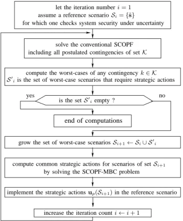
Figure 1 shows the flowchart of the proposed approach. Notice that, due to the infinite number of possible uncer-tainty patterns and the non-convex nature of the optimization problems that are tackled, our approach can not guarantee that optimal strategic actions will be found after a finite number of iterations that would guarantee safe operation with respect to the full set of initially postulated scenarios. Nevertheless, at each iteration the strategic control actions determined lead to a more secure strategy than at the previous iteration (e.g. starting up a power plant generally enhances security by providing 4In order to identify problem infeasibility we use a classical approach
which consists in relaxing the post-contingency constraints using positive slack variables and minimizing the sum of these slack variables. Strictly positive slack variables at the optimum of this problem indicate the constraints responsible for the infeasibility of the original problem.
yes no
compute common strategic actions for scenarios of setSi+1 compute the worst-cases of any contingency k∈ K
for which one checks system security under uncertainty let the iteration number i= 1
including all postulated contingencies of setK
solve the conventional SCOPF assume a reference scenarioSi= {˜s}
is the setS′ iempty ?
end of computations
by solving the SCOPF-MBC problem
implement the strategic actions up(Si+1) in the reference scenario
S′
iis the set of worst-case scenarios that require strategic actions
grow the set of worst-case scenariosSi+1← Si∪ S′i
increase the iteration count i← i + 1
Fig. 1. Flowchart of the proposed approach.
an additional degree of freedom), thus yielding an anytime optimization framework for day-ahead risk management.
IV. NUMERICAL SIMULATION RESULTS A. Results using the Nordic32 system
We consider a variant of the “Nordic 32” system shown in Fig. 2 [16]. The system contains 60 buses, 23 generators, 57 lines, 22 loads, 14 shunts, 27 transformers with fixed ratios, and 4 transformers with variable ratios.
B. Problem definition and simulation assumptions
The detailed formulation of our problem is provided in Ap-pendix B. We consider generator startups as strategic decisions to be decided in operation planning and generation re-dispatch as preventive/corrective actions. We thus seek to minimize the cost of generators that must be started up in order to enable system controllability for the next day with respect to thermal overloads. The set of strategic operation planning actions is composed of 7 initially non-dispatched generators that could be asked to run the next day (namely g2, g3, g4, g16, g17b, g19, and g21).
Table I shows the range of allowed preventive actions (PA), as up/down deviations with respect to the classical SCOPF settings, corrective actions (CA), as up/down deviations with respect to the pre-contingency state, and strategic actions (SA) in the form of the generator’s physical active power range.
Uncertainty consists in variable active and reactive power injections at any load bus, modeled by constraints (10)-(11), in the range of -5% to +5% of the nominal active/reactive
1022 g11 g12 g13 g10 g9 g21 g22 g20 g19 g6 g16 2032 11 4042 SOUTH NORTH 4062 4045 4051 4047 1044 1043 4061 4063 1041 1045 1042 4041 4072 4071 4021 4022 4031 4032 4044 4043 4046 cs 2031 1021 1013 1014 1012 1011 4012 4011 g17 g17b g18 g15 g8 g14 g4 g1 g5 g3 g2 g7 400 kV 220 kV 130 kV synchronous condenser CS
Fig. 2. The modified Nordic32 test system. TABLE I
RANGE OF GENERATION RESCHEDULING(MW)AS PREVENTIVE, CORRECTIVE,AND STRATEGIC ACTIONS
generator g1 g5 g6 g7 g8 g9 g10 PA (uo) 47.3 31.2 36.8 25.0 63.4 59.1 47.3 CA (uc) 20 30 10 generator g11 g12 g14 g15 g17 g18 g20 PA (uo) 37.4 37.8 41.4 184.0 47.3 35.5 59.1 CA (uc) 40 10 10 generator g2 g3 g4 g16 g17b g19 g21 SA (up) 540 630 540 600 720 540 560
load. Furthermore, the total variation of uncertain active (resp. reactive) power injections, modeled by constraints (12)-(13), is trimmed to the range +/- 1 MW (resp. MVar).
We consider a list of 33 N-1 contingencies. The following simulation cases are considered:
• case 0: the contingency is simulated at the classical
SCOPF solution by a power flow program (hence without considering any corrective action);
• case WP: the worst uncertainty pattern (WP)
correspond-ing to the contcorrespond-ingency, computed as detailed in Ref. [11];
• case WP+CA: the worst uncertainty pattern
correspond-ing to the contcorrespond-ingency considercorrespond-ing corrective actions (CA), computed as detailed in Ref. [11];
• case WP+PA+CA: the worst scenario corresponding to
the contingency considering both preventive and correc-tive controls, computed as detailed in Ref. [11];
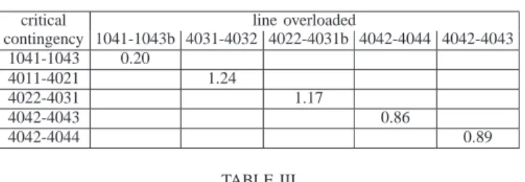
TABLE II
LINE OVERLOAD(PU)IN THE WORST PATTERN OF CRITICAL CONTINGENCIES AT THE FIRST ITERATION OF THE ALGORITHM
critical line overloaded
contingency 1041-1043b 4031-4032 4022-4031b 4042-4044 4042-4043 1041-1043 0.20 4011-4021 1.24 4022-4031 1.17 4042-4043 0.86 4042-4044 0.89 TABLE III
OVERALL LINE OVERLOAD(PU)FOR CRITICAL CONTINGENCIES FOR VARIOUS CASES DURING THE ITERATIONS OF THE ALGORITHM
case
critical 0 WP WP+CA WP+CA WP+CA
contingency +PA +PA+SA
it. 1 it. 2 it. 1 it. 2 it. 1 it. 2 it. 1 it. 2 it. 1 it. 2 1041-1043 0.02 0.00 0.20 0.12 0.18 0.10 0.14 0.00 0.00 -4011-4021 0.19 0.00 1.24 0.94 1.02 0.71 0.00 0.00 - -4022-4031 0.18 0.00 1.17 0.72 0.98 0.46 0.00 0.00 - -4042-4043 0.16 0.00 0.86 0.51 0.57 0.19 0.00 0.00 - -4042-4044 0.19 0.08 0.89 0.78 0.60 0.22 0.00 0.00 -
-SCOPF-MBC problem which includes the worst case for a single contingency and considers strategic actions (SA), preventive actions and corrective actions.
For the sake of illustration of our approach, all line current limits have been decreased by 50%, e.g. they are set to 700 MVA, or 7 pu (resp. 175 MVA, or 1.75 pu) on the 400kV (resp. 130kV) voltage level.
C. Illustration of the approach
We first compute a reference schedule for the nominal sce-nario by minimizing generation cost with a classical SCOPF formulation [15] including the 33 contingencies and relying on the preventive and corrective actions provided in Table I.
At this SCOPF optimum we compute the worst uncertainty pattern for each contingency with respect to thermal overloads, using the approach presented in [11]. We notice that only 5 out of 33 contingencies are critical i.e. they lead to overloads for their worst uncertainty pattern (case WP). Table II provides the lines overloaded by the worst pattern of each critical contingency at the first iteration of the algorithm.
Table III summarizes the results of the main steps of the approach. Notice that at the first iteration of the algorithm (col-umn denoted with “it. 1”): neither contingency is controllable by corrective actions only, 4 contingencies are controllable by appropriate combinations of preventive and corrective actions, and one contingency (1041-1043) requires strategic actions. The latter are computed by solving the SCOPF-MBC problem which includes the reference scenario and the five worst-cases of critical contingencies and, for each of them, the whole set of postulated contingencies. The solution of this SCOPF-MBC problem indicates as strategic action that generator g17b must be started up and should produce 269 MW.
At the second iteration a new reference operation schedule ˜
uo is computed by solving the conventional SCOPF while
assuming that the generator g17b is started up. From this reference situation, the whole analysis is carried out again,
to check feasibility of secure operation by trying to identify new worst-case scenarios.
We observe that the strategic action of requesting the start-up of g17b has a beneficial impact for all contingencies since the amount of overload is lower in all cases at the second iteration. Because all contingencies can now be covered (even in their worst case scenario) only with preventive and corrective actions the algorithm’s fixed point is reached.
D. Infeasible relaxations of the SCOPF-MBC problem The proposed approach may lead to consider very extreme operating conditions where it may be impossible to satisfy all postulated constraints; hence some SCOPF-MBC sub-problems may be prone to infeasibility (see Section III-D). We highlight hereafter some potential problems that the proposed approach may encounter and discuss ways to deal with them. To this end we reduce by 10% the amount of each preventive action shown in Table I.
The amount of overload on the worst-case is provided in column WP (it. 1) on Table III. However, due to the smaller amount of preventive actions two contingencies now require strategic actions, namely contingency 1041-1043 (resp. 4022-4031) requires starting up generator g17b (resp. g19) which must produce 280.7 MW (resp. 439.6 MW).
1) On the need to include into SCOPF-MBC problem also worst-cases of preventively controllable contingencies: Before discussing the infeasible cases of various SCOPF-MBC relaxations we present an example supporting our choice to include into the SCOPF-MBC problem also worst-cases of preventively controllable contingencies.
Let us consider the critical contingency 4011-4021 for which there exist preventive actions (and appropriate contingency-dependent corrective actions) to cover its worst-case (see section III-B).
However, we notice that the SCOPF problem for this worst-case, described at step 3 of the algorithm of section III-B, including the 31 contingencies (contingencies 1041-1043 and 4022-4031 that need strategic actions have been removed) is infeasible. We have identified 2 contingencies responsible for infeasibility namely: 4046-4047 and 4043-4047. These two contingencies are conflicting with 4011-4021. Although the worst case for 4046-4047 and 4043-4047 does not lead to overloads (the largest loading being around 97 %) the preventive actions to cover contingency 4011-4021 (e.g. g15 increases its output with 128 MW to remove the overload due to contingency 4011-4021) leads to post-contingency overload of line 4046-4047 (of 0.80 pu, for contingency 4043-4047) and of line 4043-4047 (of 0.84 pu, for contingency 4046-4047).
Furthermore, the SCOPF-MBC problem including the 31 contingencies for this worst-case is feasible and proposes as strategic action to start up the generator g17b.
2) Infeasibility of relaxation R-1S of the SCOPF-MBC: Let us consider the contingency 4022-4031. The solution of the SCOPF-MBC problem for the worst-case of this contingency indicates that generator g19 must be started up and produce 439.6 MW. Nevertheless, we notice that at the solution of the SCOPF-MBC problem two contingencies lead to very large
overloads: contingency 4045-4062 (resp. 4061-4062) leads to an overload of line 4061-4062 (resp. 4045-4062) with 2.51 pu (resp. 2.89 pu). However, these contingencies are harmless in their worst-cases. As can be seen from Fig. 2 these are conflicting contingencies, since only these two lines carry the power from generator g19 to the rest of the network, and hence the SCOPF-MBC problem, which includes them beside contingency 4022-4031 is infeasible. To carry on the algorithm they must be removed from the contingency list.
3) Infeasibility of relaxation R-S-C of the SCOPF-MBC: Although there exist strategic actions to cover the worst-case of contingency 1041-1043 and 4022-4031 separately, the SCOPF-MBC problem including only both base cases and both contingencies is infeasible. The latter is owing to the generator that to be started up for one contingency is detrimental to another contingency and vice-versa. Therefore a choice, according to appropriate criteria, concerning which contingency to further cover is required.
4) Infeasibility of the whole SCOPF-MBC: By further re-laxing with 5% the bounds on preventive actions we notice that there exist strategic actions (e.g. g17b and g19 are started up and produce 224 MW and 108 MW respectively) to cover both contingencies that require strategic actions (1041-1043 and 4022-4031). Nevertheless the SCOPF-MBC problem which includes the 6 scenarios (the reference one and the 5 worst-cases) and all postulated 33 contingencies is infeasible, except if one removes contingencies 4061-4062 and 4045-4062.
5) Remarks: These infeasible cases highlight the impor-tance of choosing realistic bounds on uncertain power injec-tions. These cases also illustrate that during the procedure one may have to compute control actions which ensure the security only with respect to a maximum number of postulated contingencies. The consequences of contingencies not covered by this approach can be straightforwardly assessed at the end of the procedure, as explained in Section III-D.
E. Results using the 1203-bus system
We consider a modified planning model of the RTE5 (the
French TSO) system composed of 1203 buses, 177 generators, 767 loads, 1394 lines, 403 transformers, and 11 shunts.
F. Simulation assumptions
We again use the problem formulation of Appendix B. The set of strategic actions is composed of 21 initially non-dispatched generators for the next day. Preventive controls involve 124 generators (among the 156 dispatched ones) and consist in up/down deviations of their active power up to ∆P0
i = 0.25P max
gi . Corrective actions concern 38 generators
and consist in up/down their active power with respect to their pre-contingency state up to∆Pk
i = 0.10(P max gi − P
min gi ).
Uncertain scenariosS consist in variable active/reactive power injections at 245 significant load buses, modeled by con-straints (10)-(11), in the range of +/-10% of the nominal ac-tive/reactive load. Furthermore, the total variation of uncertain 5Note that our computations do not necessarily represent the current or past
operational practice in RTE.
TABLE IV
OVERALL LINE OVERLOAD(PU)FOR CRITICAL CONTINGENCIES FOR VARIOUS CASES DURING THE ITERATIONS OF THE ALGORITHM
critical case
contingency WP WP+CA+PA WP+CA+PA+SA
it. 1 it. 2 it. 3 it. 1 it. 2 it. 3 it. 1 it. 2 it. 3 C1 4.66 4.64 4.16 1.49 1.25 0.00 0.00 0.00 -C2 11.7 11.3 13.1 1.39 0.00 0.00 0.00 0.00 -C3 2.33 1.55 1.58 0.13 0.00 0.00 0.00 -
-active/reactive power injections, modeled by constraints (12)-(13), is trimmed to the range +/- 100 MW/MVar. We consider a contingency set K of 1029 line outages.
G. Strategic actions to cover the contingencies worst-cases Note first that during the application of our procedure only three contingencies denoted hereafter C1, C2, and C3 require strategic actions at some iterations of the algorithm.
We first compute a reference schedule for the nominal sce-nario by minimizing generation cost with a classical SCOPF formulation [15] including only 9 properly selected contingen-cies and notice that only contingencontingen-cies C1 and C2 are binding at the optimum.
At this SCOPF optimum we compute the worst uncertainty pattern for each contingency with respect to thermal overloads. Columns labelled “it. 1” in Table IV provide the overall line overload (pu) for these critical contingencies in various cases (see IV-B). Column labelled “iteration 1, all” of Table V pro-vides the strategic actions needed to cover the worst patterns of critical contingencies as the solution of the SCOPF-MBC problem. This solution indicates that five generators have to be started up.
A new reference schedule is computed with a classical SCOPF formulation which takes into account these strategic actions. Columns labelled “it. 2” in Table IV shows that these strategic actions enhance the system security very little as regards the worst overloads. This is due to fact that the cost of generators drive naturally the SCOPF solution to the thermal limit for contingency C2 and very near to the thermal limit of contingency C1. On the other hand these strategic actions provide a larger flexibility of the preventive generation re-dispatch enhancing thereby the controllability of the system. In consequence at the second iteration only contingency C1 requires further strategic actions as shown in column labeled “iteration 2” in Table V. Note that because the strategic actions required to cover contingency C1 (i.e. G1 and G9) are conflicting with the constraints of contingency C2 the overall SCOPF-MBC solution leads finally to start up five new generators in order to cover all contingencies, as shown in column labelled “iteration 2, all”.
A new reference schedule is computed with a classical SCOPF formulation which takes into account these new strate-gic actions. Even if, for reasons explained previously, the worst overload for contingency C2 is larger than at the previous iteration, the current reference schedule covers all worst-case scenarios only by combinations of preventive and corrective actions and the algorithm hence reaches its fixed point.
TABLE V
MUST RUN GENERATORS POWER(MW)AT VARIOUS ITERATIONS OF THE ALGORITHM
gen iteration 1 iteration 2
C1 C2 C3 all C1 C2 C3 all G1 578.2 256.9 G3 543.2 G7 44.4 130.5 G9 168.0 257.9 257.9 G10 294.8 299.6 G14 257.9 257.9 G16 21.3 G17 42.7 G20 63.4 68.3 G21 63.4 68.3
H. Computational effort of the approach
The average computational effort for each task of our approach obtained on a PC Pentium IV (1.9-GHz, 2-GB RAM) for the 1203-bus system is as follows:
• the classical SCOPF to compute a reference schedule including 9 contingencies takes around 391 seconds;
• the OPF to compute the worst-pattern for a given set of violated constraints takes around 3 seconds;
• the NLP SCOPF-MBC including 3 (resp. 5) worst cases and 3 contingencies takes around 410 (resp. 2008) sec-onds;
• the security analysis of the full set of 1029 contingencies lasts around 307 seconds.
The MILP problem stemming from the DC approximation of the SCOPF-MBC (see Appendix C) including 3 (resp. 4) base cases and 3 (resp. 9) contingencies takes around 19 (resp. 278) seconds on a computer with 1.86-GHz, 8-GB RAM.
Note that our implementation did not exploit any parallel computations (inherent to some processes such as the security analysis, computation of the worst-case for various contin-gencies) and has also not been particularly optimized for computational speed. Furthermore, the TSO expertise can be very useful to filter-out harmless constraints in the worst-case computation (e.g. by the a priori knowledge of the weak-points of the grid) and reduce the set of postulated contingencies.
Nevertheless, these computing times suggest that the ap-proach is computationally intensive but certainly feasible in day-ahead framework for systems of realistic sizes.
V. CONCLUSIONS AND FUTURE WORKS
In this paper we have proposed an algorithmic approach for computing day-ahead operation planning decisions in order to render feasible next day security management for a range of possible operating conditions representing the uncertainties faced by operation planners.
In our work, the uncertainty about the next day operation is initially represented as an infinite (convex) set of possible power injection scenarios. Based on this information, we construct iteratively a finite approximation of this uncertainty set, yielding an anytime algorithm computing at each iteration a more robust operation plan for the next day, in the sense that it covers a larger set of extreme scenarios than the plans produced at the previous iterations. At the intermediate steps,
many surrogate optimization problems are solved in order to determine further extreme scenarios in a way driven by a constraint/contingency wise analysis. An important outcome of the approach is also the identification of cases where no strategic action has to be taken in order to cover all worst-cases during the next day by preventive/corrective controls.
From a practical application point of view, the TSO must be aware as early as possible of the strategic actions that would be necessary to cover the operation planning horizon of say 24 to 48 hours, but she/he would postpone as much as possible the last moment of their implementation (e.g. according to the minimum notification time required to start up a unit), so as to possibly take advantage of the reduction of uncertainties as time passes. Hence these analyses have to be made in a receding time horizon fashion.
While the computations performed in our approach may benefit from modern high-performance parallel computing architectures, further research will look at more efficient con-straint relaxation schemes, in particular by further untangling the relaxations along uncertain injection scenarios and along contingency sets.
Future work should be devoted to more sophisticated uncer-tainty models, addressing in particular the correlation between exogenous perturbations.
On the longer term, we think that the proposed approach is also a basis to develop a rational and practical risk-based approach to day-ahead security management, with the goal of minimizing the costs of day-ahead and real-time operation decisions while constraining the probability of insecure oper-ation, for example along the ideas proposed in [18]. Within this context, a fruitful line of investigation would be to take advantage of recent progress in the context of multi-stage stochastic programming, especially as concerns the optimal generation of scenario trees of limited size [19].
Another relevant development of our work is to couple in a multi-period optimization framework the generators that need to be started-up to enhance system security for different periods of time of the next day [20], while taking into account temporal correlations of uncertain scenarios.
If the market environment allows the intrusion into the solu-tion of the unit committment our formulasolu-tion can be naturally extended to take also into account units de-commitment [17] at the expense of an increase of the computational effort of some tasks of the approach such as the MILP approximation and the NLP relaxations.
APPENDIX
A. Worst scenario with respect to a contingency
The computation of worst scenario with respect to a contin-gency can be made using the following SCOPF that includes the base case constraints as well as constraints for the contin-gency of concern: max Pu,Qu X ij∈VC Iijk(Vik, Vjk, θki, θkj) (9) subject to:
Pmin ui ≤ Pui≤ Puimax, ∀i ∈ N (10) Qmin ui ≤ Qui≤ Qmaxui , ∀i ∈ N (11) Pumin≤ X i∈N fP iPui≤ Pumax (12) Qmin u ≤ X i∈N fQiQui ≤ Qmaxu (13) P0 gi− Pli+ fP iPui− X j∈B0 i P0 ij(V 0 i , V 0 j, θ 0 i, θ 0 j) = 0, ∀i ∈ N (14) Q0 gi− Qli+ fQiQui− X j∈B0 i Q0 ij(V 0 i , V 0 j, θ 0 i, θ 0 j) = 0, ∀i ∈ N (15) Qmin gi ≤ Q 0 gi≤ Q max gi , ∀i ∈ G (16) I0 ij(V 0 i , V 0 j, θ 0 i, θ 0 j) ≤ I max 0 ij , ∀i, j ∈ N (17) Vmin 0 i ≤ V 0 i ≤ V max 0 i , ∀i ∈ N (18) Pk gi− Pli+ fP iPui− X j∈Bk i Pk ij(Vik, Vjk, θik, θkj) = 0, ∀i ∈ N (19) Qkgi− Qli+ fQiQui− X j∈Bk i Qkij(Vik, Vjk, θki, θkj) = 0, ∀i ∈ N (20) Qmin gi ≤ Qkgi≤ Q max gi , ∀i ∈ G, (21)
where, superscript 0 (resp. k) refers to the base case (resp. contingency k state), Pui and Qui denotes uncertain active
and reactive power injections at bus i, fP i, fQi ∈ {0, 1}
are coefficients indicating buses where power injections are uncertain (i.e. fP i = 1 or fQi= 1), N is the set of buses, G
is the set of generators,Biis the set of branches connected to
busi, the other notations being self-explanatory.
Uncertain injections are limited at each individual bus by constraints (10) and (11) as well as overall by constraints (12) and (13).
The objective (9) aims at maximizing the overload of the branches of set VC. The branches of this set are identified in a combinatorial fashion as explained in [11] and hence the above problem may need to be solved several times.
Note that pre-contingency constraints (14)-(18) may be removed from this formulation since they are often less restrictive than post-contingency constraints. In this case the problem is reduced to an OPF that optimizes a single post-contingency state.
B. Detailed problem formulation
The proposed approach to the day-ahead operational plan-ning problem (1)-(8) can be formulated in more mathematical details as follows: min Pgip,P 0,s gi ,P k,s gi ,δi X i∈Up δi(c0,i+ c1,iPgip) (22) subject to: Pgi0,s− Pli− X j∈B0 i Pij0,s(V 0,s i , V 0,s j , θ 0,s i , θ 0,s j ) + δiPgip + Puis = 0, ∀i ∈ N , ∀s ∈ S (23) Q0gi,s− Qli− X j∈B0 i Qij0,s(Vi0,s, Vj0,s, θ0i,s, θ0j,s) + δiQpgi+ Qsui= 0, ∀i ∈ N , ∀s ∈ S (24) Iij0,s(Vi0,s, Vj0,s, θ0,si , θ0,sj ) ≤ Imax 0 ij , ∀i, j ∈ N , ∀s ∈ S (25) Vmin 0 i ≤ V 0,s i ≤ V max 0 i , ∀i ∈ N , ∀s ∈ S (26) Pmin gi ≤ P 0,s gi ≤ P max gi , ∀i ∈ G, ∀s ∈ S (27) Qmin gi ≤ Q 0,s gi ≤ Q max gi , ∀i ∈ G, ∀s ∈ S (28) δiPgimin≤ P p gi≤ δiPgimax, ∀i ∈ Up (29) δiQmingi ≤ Q p gi≤ δiQmaxgi , ∀i ∈ Up (30) Pgik,s− Pli− X j∈Bk i Pijk,s(Vik,s, Vjk,s, θk,si , θjk,s) + δiPgip + Puis = 0, ∀i ∈ N , ∀k ∈ K, ∀s ∈ S (31) Qk,sgi − Qli− X j∈Bk i Qk,sij (Vik,s, Vjk,s, θik,s, θk,sj ) + δiQpgi+ Qsui= 0, ∀i ∈ N , ∀k ∈ K, ∀s ∈ S (32) Iijk,s(Vik,s, Vjk,s, θk,si , θjk,s) ≤ Imaxk ij , ∀i, j ∈ N , ∀k ∈ K, ∀s ∈ S (33) Vmink i ≤ V k,s i ≤ V maxk i , ∀i ∈ N , ∀k ∈ K, ∀s ∈ S (34) Pmin gi ≤ Pgik,s≤ P max gi , ∀i ∈ G, ∀k ∈ K, ∀s ∈ S (35) Qmin gi ≤ Q k,s gi ≤ Q max gi , ∀i ∈ G, ∀k ∈ K, ∀s ∈ S (36) |Pgi0,s− ˜P0 gi| ≤ ∆P 0 i, ∀i ∈ G, ∀s ∈ S (37) |Pgik,s− Pgi0,s| ≤ ∆Pik, ∀i ∈ G, ∀k ∈ K, ∀s ∈ S (38) δi∈ {0, 1}, ∀i ∈ Up (39)
where, superscript 0 (resp. k) refers to the base case (resp. contingencyk state), S is the set of scenarios, K is the set of postulated contingencies,G is the set of dispatched generators, N is the set of buses, Biis the set of branches connected to bus
i, Upis the set of strategic actions (i.e. initially non-dispatched
generators),c0,iandc1,iare the start up cost and the operation
cost of generatori, δi is a binary variable indicating whether
the initially non-dispatched generatori is started up or not, Pgip (resp.Qpgi) is the active (resp. reactive power) of the generator that can be started up at bus i, hence the vector of strategic actions up is composed by (Pgip, Q
p
gi), i ∈ Up, any scenario
s is defined by a particular pattern of uncertain injections (Ps
ui, Qsui), ∀i ∈ N that satisfies constraints (10)-(13) which
defines the setS, the other notations being self-explanatory. C. Solving the MINLP problem by a heuristic combining MILP and NLP
Notice that due to the presence in the problem formulation of binary variables modeling strategic actions (such as gen-erator start up) our problem is a Mixed Integer NonLinear Program (MINLP), which also inherits challenging features of the underlying SCOPF model such as non-convex and very
large-scale nature. Furthermore, such a MINLP problem has to be solved in a sequential loop, together with other tasks, and where the number of iterations is unknown beforehand (see section III-A). Given the extreme difficulty of the whole approach for which a reasonable solution is needed in a bounded time frame, the experience we acquired with various MINLP solvers [17] suggest that, letting aside their huge memory requirements, nowadays they can not meet practical response time requirements in the case of realistic power system sizes.
For these reasons one needs to rely on heuristic techniques to solve this MINLP problem. To this end we implemented an algorithm that combines the resolution of a MILP problem with a sequence of NLP problems, as detailed hereafter.
The proposed algorithm contains the following steps: 1) Solve the MILP approximation of the original problem
(22)-(39) relying on the DC model. Let the set UO p
denote the generators fromUp for whichδi = 1 at the
MILP solution, and letUR
p = Up\ UpO.
2) Solve the NLP problem (22)-(39) whereδi= 0, i ∈ UpR
andδi= 1, i ∈ UpO.
If this NLP problem is feasible then an acceptable solution of the original MINLP problem is obtained and computations end.
3) Otherwise, solve an NLP relaxation of the original prob-lem (22)-(39) whereδi= 1, i ∈ UpR,δi= 1, i ∈ UpO, and
the constraints of the generators in setUR
p are relaxed to0 ≤ Pgip ≤ Pmax gi . a) IfPgip = 0 ∨ Pgip ∈ [Pmin gi , P max gi ], ∀i ∈ UpRthen an
acceptable solution of the original MINLP problem is obtained and computations end.
b) If ∃i ∈ UR p such that P p gi ∈ [P min gi , P max gi ] add to the set UO
p the generators for which P p gi ∈ [Pmin gi , P max gi ] and adjust UpR toUp\ UpO. Go to step 2.
c) Rank the generators of setUR
p in decreasing order
of their relative distance to the minimal bound Pgip/Pmin
gi .
d) Pick the top6 ranked generator j and let UR p ←
UR
p \ {j} and UpO← UpO∪ {j}.
Go to step 2.
Observe that if the very first set of strategic actions com-puted by the MILP algorithm proves being insufficient by the NLP at the second step, then the algorithm solves a sequence of NLPs which aim at starting up an increasing number of generators until the NLP becomes feasible.
Note also that in the NLP relaxation at step 3 we approxi-mate the cost function of an initially non-dispatched generator, that mixes-up the start up cost c0,iand its operation costc1,i,
by a quadratic function over the range [0, Pmax
gi ]. We also
assume that generators of set UR
p produce no reactive power
i.e. Qpgi= 0.
In order to illustrate our approach, we use the solver Xpress-Mosel [22] to solve the MILP problem and the multiple 6More aggressive strategies could be used, e.g. like a round-off technique,
depending on the time allowed to solve the problem.
centrality corrections interior-point algorithm [23] to solve the NLP problems.
Our iterative algorithm involves among others the successive solutions of various NLP problems. While some efficient NLP solvers rely on warm starts of successive solutions from the previous one, the interior point method does not naturally warm start well. Nevertheless, we look forward to assess for power systems optimization problems the significant improve-ments on the warm start ability of interior point methods reported for generic NLPs [21]. Other codes that have proven their efficiency on many practical applications such as the sequential linear programming approach of [5] could also be used in our framework.
ACKNOWLEDGMENTS
This paper presents research results of the European FP7 project PEGASE funded by the European Commission.
Louis Wehenkel and Florin Capitanescu also acknowledge the support of the Belgian Network DYSCO (Dynamical Systems, Control, and Optimization), funded by the Interuni-versity Attraction Poles Programme, initiated by the Belgian State, Science Policy Office. The scientific responsibility rests with the authors.
We also wish to thank Brian Stott and the anonymous reviewers of this paper for their thoughtful comments and suggestions.
REFERENCES
[1] A. Gomez-Exposito, A. Conejo, C. Canizares (Eds.), “Electric Energy Systems: Analysis and Operation”, CRC Press, 2009.
[2] H. Pinto, F. Magnago, S. Brignone, O. Alsac, B. Stott, “Security constrained unit commitment: network modeling and solution issues”,
IEEE PSCE conference, 2006, pp. 1759-1766.
[3] Y. Fu, M. Shahidehpour, Z. Li, “AC contingency dispatch based on security-constrained unit commitment”, IEEE Trans. Power Syst., vol. 21, no. 2, 2006, pp. 897-908.
[4] P.A. Ruiz, C.R. Philbrick, E. Zak, K.W. Cheung, P.W. Sauer, “Uncer-tainty Management in the Unit Commitment Problem”, IEEE Trans.
Power Syst., vol. 24, no. 2, 2009, pp. 642-651.
[5] O. Alsac, J. Bright, M. Prais, and B. Stott, “Further developments in LP-based optimal power flow”, IEEE Trans. Power Syst., vol. 5, no. 3, 1990, pp. 697-711.
[6] J. Jarjis, F.D. Galiana, “Quantitative analysis of steady state stability in power networks”, IEEE Trans. on Power Apparatus and Systems, vol. PAS-100, no. 1, 1981, pp. 318-326.
[7] D. Gan, X. Luo, D.V. Bourcier, R.J. Thomas, “Min-Max Transfer Ca-pability of Transmission Interfaces”, International Journal of Electrical
Power and Energy Systems, vol. 25, no. 5, 2003, pp. 347-353.
[8] I. Dobson, L. Lu, “New methods for computing a closest saddle node bifurcation and worst case load power margin for voltage collapse”,
IEEE Trans. on Power Systems, vol. 8, no. 2, 1993, pp. 905-911.
[9] F. Capitanescu, T. Van Cutsem, “Evaluating bounds on voltage and thermal security margins under power transfer uncertainty”, Proc. of
the PSCC Conference, Seville (Spain), June 2002.
[10] P. Panciatici, Y. Hassaine, S. Fliscounakis, L. Platbrood, M. Ortega-Vazquez, J.L. Martinez-Ramos, L. Wehenkel, “Security management under uncertainty: from day-ahead planning to intraday operation”, Proc.
of the IREP Symposium, Buzios (Brazil), 2010.
[11] F. Capitanescu, S. Fliscounakis, P. Panciatici, and L. Wehenkel, “Day-ahead security assessment under uncertainty relying on the combination of preventive and corrective controls to face worst-case scenarios”, Proc.
of the PSCC Conference, Stockholm (Sweden), August 2011. Available
on-line at: http://orbi.ulg.ac.be/simple-search?query=capitanescu. [12] R. Zimmeman, “A superOPF framework”, presentation at FERC
Con-ference on Enhanced Optimal Power Flow Models, Washington, USA,
[13] B. Colson, P. Marcotte, G. Savard, “An overview of bilevel optimiza-tion”, Annals of Operations Research, vol. 1, 2007, pp. 235-256. [14] J. M. Arroyo, F. D. Galiana, “On the solution of the bilevel programming
formulation of the terrorist threat problem”, IEEE Trans. on Power
Systems, vol. 20, no. 2, May 2005, pp. 789-797.
[15] F. Capitanescu, L. Wehenkel, “A new iterative approach to the corrective security-constrained optimal power flow problem”, IEEE Trans. on
Power Systems, vol. 23, no.4, November 2008, pp. 1342-1351.
[16] Nordic32 system, CIGRE Task Force 38.02.08, “Long-term dynamics, phase II”, 1995.
[17] L. Platbrood, S. Fliscounakis, F. Capitanescu, P. Panciatici, C. Merckx, and M. Ortega-Vazquez, “Deliverable D3.2: development of prototype software for system steady-state optimization of the European trans-mission system”, PEGASE project, available on-line at http://www.fp7-pegase.eu/, 2011.
[18] P.P. Varaiya, F.F. Wu, J.W. Bialek, “Smart operation of smart grid: risk-limiting dispatch”, Proceedings of the IEEE, Vol. 99, No. 1, January 2011, pp. 40-57.
[19] B. Defourny, D. Ernst, L. Wehenkel, “Multistage stochastic program-ming: a scenario tree based approach to planning under uncertainty”, to appear in Decision Theory Models for Applications in Artificial
Intelligence: Concepts and Solutions, L. Enrique Sucar, Eduardo F.
Morales, and Jesse Hoey eds., IGI Global, 2011, 51 pages.
[20] E. Lobato, L. Rouco, T. Gomez, F. Echavarren, M. Navarrete, R. Casanova, G. Lopez, “A Practical Approach to Solve Power System Constraints With Application to the Spanish Electricity Market”, IEEE
Trans. Power Syst., vol. 19, no. 4, 2004, pp. 2029-2037.
[21] H.Y. Benson and D.F. Shanno, “Interior-point methods for nonconvex nonlinear programming: regularization and warmstarts”, Computational
Optimization and Applications, vol. 40, no. 2, 2008, pp. 143-189.
[22] Solver Xpress-mosel v2.2.2, http://www.fico.com/en/Products/DMTools/ xpress-overview/Pages/Xpress-Mosel.aspx.
[23] F. Capitanescu, M. Glavic, D. Ernst, and L. Wehenkel, “Interior-point based algorithms for the solution of optimal power flow problems”,
Electric Power Syst. Research, vol. 77, no. 5-6, April 2007, pp.
508-517.
Florin Capitanescu graduated in Electrical Power Engineering from the
University “Politehnica” of Bucharest (Romania) in 1997. He obtained the Ph.D. degree from the University of Li`ege in 2003. His main research interests lie in the field of power systems operation, planning, and control, with particular emphasis on optimization methods and voltage stability.
St´ephane Fliscounakis received the M.Sc. degree in Applied Mathematics
from Universit´e Paris Pierre et Marie Curie and a M.Sc. degree in Industrial Automation and Control from Universit´e Paris Sud Orsay. Since 1992 he works for RTE as research engineer.
Patrick Panciatici graduated from the French Ecole Sup´erieure d’Electricit´e
in 1984. He joined EDF R&D in 1985, managing EUROSTAG Project and CSVC project. He joined RTE in 2003 and participated in the creation of the department “Methods and Support”. He is the head of a team which develops real time and operational planning tools for RTE, and ensures operational support on the use of these tools. Member of CIGRE, IEEE and SEE. Member of the R&D ENTSO-E Working Group. RTE’s representative in PSERC and several European Projects (PEGASE, OPTIMATE, TWENTIES, etc.).
Louis Wehenkel graduated in Electrical Engineering (Electronics) in 1986
and received the Ph.D. degree in 1990, both from the University of Li`ege (Belgium), where he is full Professor of Electrical Engineering and Computer Science. His research interests lie in the fields of stochastic methods for systems and modeling, optimization, machine learning and data mining, with applications in complex systems, in particular large scale power systems planning, operation and control, industrial process control, bioinformatics and computer vision.