Mercedes L´opez-Morales
Harvard-Smithsonian Center for Astrophysics, 60 Garden Street, Cambridge, MA 01238, USA
Amaury H. M. J. Triaud1
Department of Physics, and Kavli Institute for Astrophysics and Space Research, Massachusetts Institute of Technology, Cambridge, MA 02139, USA
Florian Rodler2
Max-Planck-Institut f¨ur Astronomie, K¨onigstuhl 17, D-69117 Heidelberg, Germany, Harvard-Smithsonian Center for Astrophysics, 60 Garden Street, Cambridge, MA 01238,
USA
Xavier Dumusque1
Harvard-Smithsonian Center for Astrophysics, 60 Garden Street, Cambridge, MA 01238, USA
Lars A. Buchhave
Harvard-Smithsonian Center for Astrophysics, 60 Garden Street, Cambridge, MA 01238, USA
Centre for Star and Planet Formation, Natural History Museum of Denmark, University of Copenhagen, DK-1350 Copenhagen, Denmark
Avet Harutyunyan
Fundaci´on Galileo Galilei - INAF, Rambla Jos´e Ana Fernandez P´erez, 738712 Bre˜na Baja, Tenerife, Spain
Sergio Hoyer3, Roi Alonso
Instituto de Astrof´ısica de Canarias, E-38205 La Laguna, Tenerife, Spain; Dept. de Astrof´ısica, Universidad de La Laguna, E-38206 La Laguna, Tenerife, Spain
Micha¨el Gillon
Institut d’Astrophysique et G´eophysique, Universit´e de Li`ege, All´ee du 6 Aoˆut 17, 4000 Li`ege, Belgium
Nathan A. Kaib
Center for Interdisciplinary Exploration and Research in Astrophysics (CIERA) and Department of Physics and Astronomy, Northwestern University, 2131 Tech Drive,
Evanston, IL 60208, USA David. W. Latham
Harvard-Smithsonian Center for Astrophysics, 60 Garden Street, Cambridge, MA 01238, USA
Christophe Lovis, Francesco Pepe
Observatoire Astronomique de l’Universit´e de Gen`eve, Chemin des Maillettes 51, Sauverny, CH-1290, Switzerland
Didier Queloz
Cavendish Laboratory, J J Thomson Avenue, Cambridge CB3 0HE, UK; Observatoire Astronomique de l’Universit´e de Gen`eve, Chemin des Maillettes 51, Sauverny, CH-1290,
Switzerland Sean N. Raymond
Universit´e de Bordeaux, LAB, UMR 5804, BP F-33270 Floirac, France; CNRS, LAB, UMR 5804, F-33270 Floirac, France
Observatoire Astronomique de l’Universit´e de Gen`eve, Chemin des Maillettes 51, Sauverny, CH-1290, Switzerland
Ingo P. Waldmann
Department of Physics and Astronomy, University College London, Gower Street, WC1E6BT, UK
St´ephane Udry
Observatoire Astronomique de l’Universit´e de Gen`eve, Chemin des Maillettes 51, Sauverny, CH-1290, Switzerland
Received ; accepted
1Swiss National Science Foundation Fellow 2Alexander-von-Humboldt Postdoctoral Fellow 3Severo Ochoa Fellow
ABSTRACT
We present Rossiter-McLaughlin observations of the transiting super-Earth 55 Cnc e collected during six transit events between January 2012 and November 2013 with HARPS and HARPS-N. We detect no radial-velocity signal above 35 cm s−1 (3σ) and confine the stellar v sin i? to 0.2 ± 0.5 km s−1. The star appears
to be a very slow rotator, producing a very low amplitude Rossiter-McLaughlin effect. Given such a low amplitude, the Rossiter-McLaughlin effect of 55 Cnc e is undetected in our data, and any spin–orbit angle of the system remains possible. We also performed Doppler tomography and reach a similar conclusion. Our results offer a glimpse of the capacity of future instrumentation to study low amplitude Rossiter-McLaughlin effects produced by super-Earths.
Subject headings: planets and satellites: formation — planets and satellites: individual (55 Cancri e) — stars: individual (55 Cancri) — techniques: radial velocities — techniques: spectroscopic
1. Introduction
55 Cnc is a 0.9 M star (von Braun et al. 2011) harbouring five known planets with
masses between 0.025 MJup and 3.8 MJup, and orbital periods between ∼ 0.74 days and
∼ 4872 days (Nelson et al. 2014). The star also has a ∼ 0.27 M binary companion at a
projected orbital separation of 1065 AU (Mugrauer et al. 2006).
The innermost planet in the system, 55 Cnc e (Mp = 8.3 ± 0.4 MEarth; Rp = 1.94
± 0.08 REarth), was found to transit by Winn et al. (2011) and Demory et al. (2011),
after Dawson & Fabrycky (2010) provided a revised period of 0.74 days, shorter than the originally reported 2.8 days period by McArthur et al. (2004). The presence of transits makes 55 Cnc e an invaluable potential target for future studies of atmospheric properties of super-Earths, and spin–orbit angle studies via the Rossiter-McLaughlin effect (Rossiter 1924; McLaughlin 1924; Queloz et al. 2000; Gaudi & Winn 2007). In the case of spin-orbit angle studies, a result for 55 Cnc e would add to the very few measurements reported so far for Neptune and super-Earth mass planets, e.g. the detection of oblique orbits for HAT-P-11b (Winn et al. 2010; Hirano et al. 2011), and for the multiple super-Earth systems Kepler-50 and Kepler-65 – these last two via asteroseismology (Chaplin et al. 2013). There is also the non-detection of the Rossiter-McLaughlin effect of GJ 436 by Albrecht et al. (2012), which indicates that the star is a very slow rotator with v sin i? < 0.4 km s−1.
Kaib et al. (2011) showed that the distant binary companion to 55 Cnc causes the planetary system to precess as a rigid body (see also Innanen et al. 1997; Batygin et al. 2011; Bou´e & Fabrycky 2014). The planets’ orbits nonetheless remain confined to a common plane such that a measurement of planet e’s spin-orbit angle should be representative of the entire system. Given the unknown orientation of the wide binary orbit, Kaib et al. (2011) calculated that the plane of the planets is most likely tilted with respect to the stellar equator. The plane could be tilted by virtually any angle, with a most probable projected
spin-orbit angle of ∼ 50◦ There is also a ∼ 30% chance of a retrograde configuration.
Valenti & Fischer (2005) estimated a v sin i? for 55 Cnc of 2.4 ± 0.5 km s−1, which,
combined with the depth of the observed transit, was expected to yield a Rossiter-McLaughlin effect with a semi-amplitude of 70 ± 15 cm s−1. Such an amplitude should be detectable with stabilized, high resolution spectrographs such as HARPS (Molaro et al. 2013).
Following those results we set out to detect the Rossiter-McLaughlin effect of 55 Cnc e and test the spin–orbit misalignment prediction of the system by Kaib et al. (2011).
2. Observations
Shortly after the detection of 55 Cnc e’s transit was announced, we requested four spectroscopic time series on HARPS (Prog. ID 288.C-5010; PI Triaud), as Director Discretionary Time. HARPS is installed on the 3.6-m telescope at the European Southern Observatory on La Silla, Chile (Mayor et al. 2003). The position of 55 Cnc in the sky — RA(J2000) = 08:52:35.81, Dec(J2000) = +28:10:50.95 — is low as seen from La Silla. The target remains at a zenith distance of z < 2 for only ∼ 2.5 hours per night, with a transit duration of about 1.5 hours having to fit within this tight window. This constraint on the airmass, essential to obtain precise RVs, is set by the instrumental atmospheric dispersion corrector. We used the ephemeris by Gillon et al. (2012), then at an advanced stage of preparation, to schedule our observations. In total we gathered 179 spectra on the nights starting on 2012-01-27, 2012-02-13, 2012-02-27 and 2012-03-15 UT.
The target is better suited for observations from the north and, therefore, in 2013 we acquired additional radial velocity time series with the newly installed HARPS-N instrument on the 3.57-m Telescopio Nazionale Galileo (TNG) at the Observatorio del
Roque de los Muchachos in La Palma, Spain (Cosentino et al. 2012). HARPS-N is an updated version of HARPS, and is able to reach the same overall RV precision, if not better (see e.g. Pepe et al. 2013; Dumusque et al. 2014). The HARPS-N time was awarded via the Spanish TAC (Prog. ID 34-TNG4/13B; PI Rodler) and observations were collected on the nights starting on 2013-11-14 and 2013-11-28 UT. We gathered a total of 113 spectra in those two nights. A third night awarded to this program was lost to weather. Some more details about the observations are provided in Table 1.
3. Radial-Velocity extraction
The spectra were originally reduced with version 3.7 of the HARPS and HARPS-N Data Reduction Software (DRS), which includes color systematic corrections (Cosentino et al. 2014). Radial velocities were computed using a numerical weighted mask following the methodology outlined by Baranne et al. (1996). Such a procedure has been shown to yield remarkable precision and accuracy (e.g. Mayor et al. 2009; Molaro et al. 2013; Pepe et al. 2013; Dumusque et al. 2014).
However, there is still room for improvement. A detailed analysis of the RV of individual spectral lines in HARPS spectra has revealed that some lines can show variations > 100 m s−1 as a function of time. These variations cannot be explained by stellar noise in a star like 55 Cnc. Indeed, stellar oscillations, granulation phenomena and stellar activity are expected to be of the order of a few m s−1 on a inactive G dwarf, as reported by Dumusque et al. (2011). After an in-depth study of the behavior of these lines, we identify three sources of velocity errors: the stitching of the CCD, some faint telluric lines, and fringing on the detector can all introduce significant velocity shifts of certain stellar lines that happen to fall near the stationary features, changing as the barycentric velocity for different observations scans the stellar lines across the artifacts.
The spectral lines affected by these variations were identified by calculating the periodogram of the RV of each spectral line used in the stellar template. All the spectral lines that were exhibiting a signal more significant than 10% in false alarm probability were flagged as bad lines and removed from the stellar template. The result is a modified mask, which is used instead of the standard K5 mask, to derive the RV of each observed spectrum by cross-correlation.
After performing a new cross-correlation of the data using this cleaned stellar template, the rms of the combined RV curve was reduced from 1.17 m s−1 to 1.04 m s−1. In the rest of our analysis we used the set of RV values from this revised reduction (a publication with this analysis is in preparation). Those radial velocities are presented in Table 1 and in Figure 1.
4. Estimates of line broadening due to stellar rotation
The large number of high signal-to-noise ratio (SNR) high-resolution spectra gathered by HARPS-N allowed us to re-determine the stellar parameters of 55 Cnc using the Stellar Parameter Classification pipeline (SPC; Buchhave et al. 2014). We analyzed the 55 spectra observed on the night starting on 2013-11-14 with exposure times of 240 seconds and a resolution of R = 115,000 resulting in an average SNR per resolution element of 362 in the MgB region. We also analyzed three spectra, with SNR per resolution element of 143 and resolution R = 48,000, obtained between 2013-04-22 and 2014-03-08 with the fiber-fed Tillinghast Reflector Echelle Spectrograph (TRES; Szentgyorgyi & Fur´esz 2007) on the 1.5-m Tillinghast Reflector at the Fred Lawrence Whipple Observatory on Mt. Hopkins, Arizona. The weighted average of each spectroscopic analysis yielded two sets of values from the two instruments, which are in very close agreement. The final stellar parameters are the average of these two sets, yielding Teff=5358 ± 50 K, log(g)=4.44 ± 0.10, and
[m/H]=0.34 ± 0.08. Those values agree with the values published in the literature. The HARPS-N spectra yielded a projected rotational velocity of v sin i? = 0.43 km s−1, with
a upper limit of 1.43 km s−1, and the TRES spectra gave v sin i? = 0.85 km s−1, with a
upper limit of 1.85 km s−1. Both values agree with each other, but lower than the value of 2.4 ± 0.5 km s−1 reported by Valenti & Fischer (2005).
We also computed the R0HK activity index from our spectra and derived the age and rotation period of the star following Mamajek & Hillenbrand (2008). We arrive to an age for the star of 9.3 ± 1.1 Gyr, a rotational period of Prot = 52 ± 5 days, and a log R0HK
= -5.07 ± 0.02 using the HARPS-N spectra. The analysis of the HARPS spectra yields similar results, i.e. age = 10.0 ± 1.2 Gyr, Prot = 54 ± 5 days, and a log R0HK = - 5.11 ±
0.02. Both results agree with previously published values (von Braun et al. 2011; Dragomir et al. 2014) and imply a rotational velocity slower than 1 km s−1, in agreement with our line broadening estimates.
5. Analysis of the radial-velocity data
The first step of our radial velocity analysis consisted of removing the Keplerian orbital motion signals of the five planets discovered around 55 Cnc from each of our six datasets. We used the most recent orbital solution of the system obtained by Nelson et al. (2014). As recommended by these authors, we used the planetary masses and orbital parameters from their Case 2, in which they considered the errors of RV observations taken within 10 minutes from each other to be perfectly correlated. The corrected radial velocities for each dataset are given in Table 1. Later tests using the Nelson et al. (2014) system parameters for their Case 1, and also the planetary masses and orbital parameters of the system derived by Dawson & Fabrycky (2010) in their tables 7, 8 and 10, yield similar results.
After removing the five-planet signal, we modelled the Rossiter-McLaughlin effect for the six datasets combined using the formalism of Gim´enez (2006), based on Kopal (1942), and adjusted with a Monte Carlo Markov-Chain described in Triaud et al. (2013). All parameters determined by the photometry were controlled by priors issued from two independent datasets (see Table 2). Additional priors included the planet’s period (Nelson et al. 2014), the stellar parameters (von Braun et al. 2011), and the two v sin i? values
estimated in Sect. 4. We allowed the relative mean of each time series to float in order to absorb any offset produced by slightly different epochs of stellar activity (e.g. Triaud et al. 2009). Thirteen parameters were thus used on a total of 293 data points. A noise term of 70 cm s−1 was quadratically added to all measurement errors to reach a final reduced χ2 of
0.97 ± 0.08. All priors and important results are summarized in Table 2.
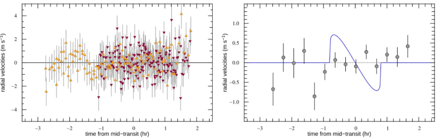
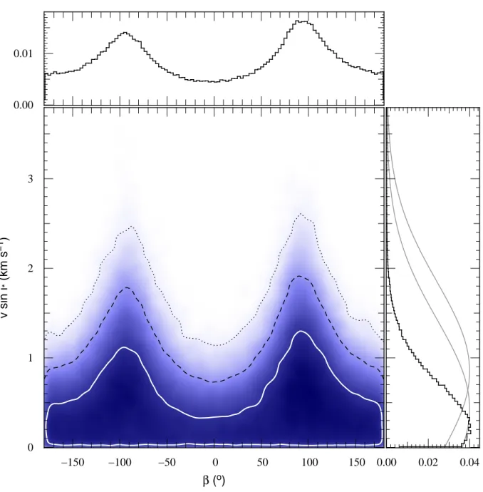
We conducted a number of different chains all converging to the same conclusion: the Rossiter-McLaughlin effect is not detected (see Figure 1). The impossibility to constrain the spin–orbit angle of the system is illustrated in Figure 2, which shows the typical crescent shape expected when there is degeneracy between fast rotation & polar orbits and slow rotation & alignment (Triaud et al. 2011; Albrecht et al. 2011). This shape approximately maps contours of Rossiter-McLaughlin effects of equal semi-amplitudes. From the 3σ contour, we rule-out Rossiter-McLaughlin effects with semi-amplitudes larger than 35 cm s−1. The fact that anti-aligned orbits are as likely as aligned orbits implies the Rossiter-McLaughlin effect is not detected.
The marginalised distribution in v sin i? is thinner and peaks closer to 0 than our
two estimates from spectral line broadening. Therefore, from the data we estimate v sin i? = 0.2 ± 0.5 km s−1. This implies the star’s most likely rotation period is 260 days
(> 22 days, with 3σ confidence; > 40 days, only considering coplanar solutions).
When replacing our two v sin i? priors with the value estimated in Valenti & Fischer
(2005), two symmetrical solutions, on polar orbits, are preferred: β = +90◦ and −90◦ (such a Rossiter-McLaughlin effect would have a semi-amplitude of 23 cm s−1). A similar situation occurred for the spin–orbit angle measurement of WASP-80b (Triaud et al. 2013), which depends entirely on the value of v sin i?. Using no priors on v sin i?, the posterior
is qualitatively similar, but both spikes are thinner and v sin i? tails to higher values, as
would be expected. The same procedures, removing the additional 70 cm s−1 noise added to the errorbars, produced similar results (with shorter confidence intervals).
6. Doppler tomography
Given the impossibility to detect the Rossiter-McLaughlin effect of 55 Cnc e, we tried to detect the signal of the planet using Doppler tomography (e.g. Albrecht et al. 2007; Collier Cameron et al. 2010). Doppler tomography reveals the distortion of the stellar line profiles when the planet, during transit, blocks part of the stellar photosphere. This distortion is a tiny dip in the stellar absorption profile, scaled down in width accordingly to the planet-to-star radius ratio. Additionally, the area of that dip corresponds to the planetary-to-stellar disks area ratio. As the planet moves across the stellar disk, the dip produces a trace in the time series of line profiles, which reveals the spin-orbit alignment between star and planetary orbit.
For this analysis we summed up all the thousands of stellar absorption lines in each spectrum into one high S/N mean line profile. For this step, we employed a least-squares deconvolution (LSD; e.g. Collier Cameron et al. 2002) of the observed spectrum and theoretical lists of the stellar absorption lines from the Vienna Atomic Line Database (VALD, Kupka et al. 1999) for a star with Teft = 5200 K and log g = 4.5. The resulting
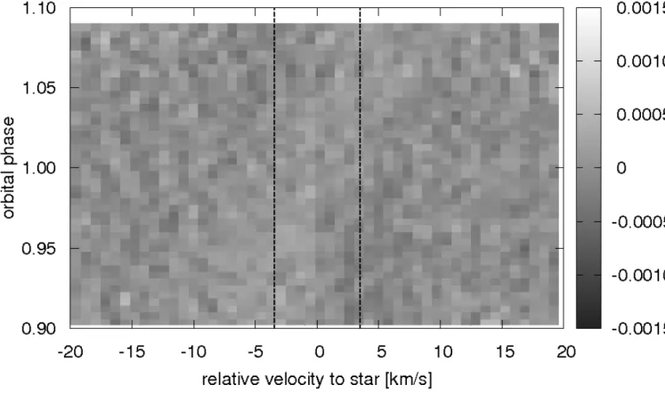
grid of 0.79 km s−1 increments, corresponding to the velocity range of one spectral pixel of HARPS-N at 550 nm. We then corrected the stellar line profiles for the radial velocity of the host star and the barycentric velocity of the Earth. For each of the six runs, we summed up all the mean line profiles collected before and after the transit and subtracted the resulting profile from the in-transit ones. We then sorted the co-aligned line profiles of all runs by orbital phase and combined the line profiles into one dataset. Figure 3 shows the residuals of the line profiles and demonstrates that we are also unable to detect a trace of the transiting planet using this method. Our ability to detect the planet using Doppler tomography is in fact limited by the resolution of the spectra (∼ 2.6 km s−1 per resolution element), given the very slow rotational velocity of the star.
7. Conclusions
Our data do not support a detection of the spectroscopic transit of 55 Cnc e, but they rule out with 3σ confidence any signal with a semi-amplitude larger than 35 cm s−1. The non-detection can be explained by one of three scenarios: either 55 Cnc rotates more slowly than the average G-K main sequence star (∼ 2.4 km s−1; Valenti & Fischer 2005), or the orbital plane of the planets is perpendicular to the equatorial plane of the star, or the spin axis of the star is highly inclined with respect to us. Dragomir et al. (2014) report no variability associated to stellar spots rotation on a 42 day continuous monitoring of 55 Cnc with MOST. von Braun et al. (2011) estimated the system age at 10.2 ± 2.5 Gyr. Therefore, the star is likely a very slow rotator, which is confirmed by our chromospheric activity measurements and stellar line broadening. Our conclusion is also consistent with a photometric modulation of 42.7 ± 2.5 days reported by Fischer et al. (2008), which they interpreted as stellar rotation. Because of the slow stellar rotation, reliably determining the projected spin–orbit angle of 55 Cnc e, or the inclination of its host’s spin axis may
remain out of reach. The slow stellar rotation also implies a weaker tidal coupling between 55 Cnc e and its host than what presumed by Bou´e & Fabrycky (2014). Following Kaib et al. (2011), that would increase the probability of a spin–orbit misalignment.
While the detection of such a misalignment currently remains out of reach, our analysis confirms the capacity of the HARPS technology to reach a few tens of cm s−1. These radial-velocity time series are the most constraining yet in precision and they reveal the suitability of HARPS and HARPS-N for follow-up and confirmation of small planets to be detected by missions like TESS. Such level of radial velocity precision will also be routinely reached by ESPRESSO on the VLT. ESPRESSO will open up the study of weak Rossiter-McLaughlin effects, produced by super-Earths transiting slow rotators such as 55 Cancri e, with the potential to see if the same diversity that has been observed in the spin–orbit angle of hot Jupiters (Triaud et al. 2010; Brown et al. 2012; Albrecht et al. 2012) also exists for small planets.
Finally, Bourrier & H´ebrard (2014) recently reported a detection of the Rossiter-McLaughlin effect of 55 Cnc e, with an amplitude of ∼ 60 cm s−1. While such radial velocity variations could be attributed to stellar surface physical phenomena (e.g. granulation or faculae), we argue that they are not produced the Rossiter-McLaughlin effect, since the necessary v sin i? ∼ 3.3 km s−1 is incompatible with the v sin i?, Prot, age, and R0HK activity
index values we measure in Sect. 4. That v sin i? is also incompatible with the ∼ 10 Gyr
stellar age derived by von Braun et al. (2011), and with the Prot > 40 days rotational period
estimates from Fischer et al. (2008) and Dragomir et al. (2014).
This publication was made possible through the support of a grant from the John Templeton Foundation. The opinions expressed are those of the authors and do not necessarily reflect the views of the John Templeton Foundation. The research leading to these results received funding from the European Union Seventh Framework Programme
(FP7/2007-2013) under Grant Agreement 313014 (ETAEARTH). This work used the VALD database, operated at Uppsala University, the Institute of Astronomy RAS in Moscow, and the University of Vienna. We thank the anonymous referee for a very constructive review and J. Winn for useful comments. A. H. M. J. T. is a Swiss National Science Foundation fellow under grant number P300P2-147773. F. R. acknowledges funding from the Alexander-von-Humboldt postdoctoral fellowship program. X. D. thanks the Swiss National Science Foundation (SNSF) for its support through an Early Postdoc Mobility fellowship. S. H. acknowledges support from the Spanish Ministry of Economy and Competitiveness under the 2011 Severo Ochoa Program MINECO SEV-2011-0187. HARPS-N is a collaboration between the Astronomical Observatory of the Geneva University, the CfA in Cambridge, the University of St. Andrews, the Queens University of Belfast, and the TNG-INAF Observatory. We thank all the researchers whose observing programs on HARPS got disrupted by our DDT program and who kindly observed for us. Finally we thank ESO’s director general, Tim de Zeeuw, who granted our HARPS observing time.
−3 −2 −1 0 1 2 −4 −2 0 2 4
time from mid−transit (hr)
radial velocities (m s −1 ) . . . . −3 −2 −1 0 1 2 −1.0 −0.5 0.0 0.5 1.0
time from mid−transit (hr)
radial velocities (m s −1 ) . . . .
Fig. 1.— Left: Radial-velocity data, in phase. HARPS data points are represented by inverted, red triangles, and HARPS-N by upright, orange triangles. Right: the same data, binned in 14 equidistant points , and a model of the Rossiter-McLaughlin effect, for v sin i? =
0.00 0.01 −150 −100 −50 0 50 100 150 0 1 2 3 0.00 0.02 0.04 v sin i * (km s −1 ) β (o)
.
.
.
.
Fig. 2.— Posterior distribution for the projection of the stellar rotational speed, v sin i?,
and the projection on the sky of the spin–orbit angle, β. 1, 2 and 3 σ confidence contours are over plotted. Side histograms display the marginalised posteriors for each quantity. In the case of v sin i?, the two priors we applied are drawn as grey lines.
Fig. 3.— Residuals of all line profiles of 55 Cnc taken during the six transits as a function of velocity and orbital phase of the planet. The two vertical dashed lines depict the area of the stellar line profile (FWHM). The units of the grey scale are fractional deviation from the average out-of-transit line profile. We are unable to detect the planetary signature in the line profiles.
REFERENCES
Albrecht, S., Reffert, S., Snellen, I., Quirrenbach, A., & Mitchell, D. S. 2007, A&A, 474, 565 Albrecht, S., Winn, J. N., Johnson, J. A., et al. 2011, ApJ, 738, 50
—. 2012, ApJ, 757, 18
Baranne, A., Queloz, D., Mayor, M., et al. 1996, A&AS, 119, 373 Batygin, K., Morbidelli, A., & Tsiganis, K. 2011, A&A, 533, A7 Bou´e, G., & Fabrycky, D. C. 2014, ApJ, 789, 111
Bourrier, V., & H´ebrard, G. 2014, ArXiv e-prints, arXiv:1406.6813
Brown, D. J. A., Cameron, A. C., Anderson, D. R., et al. 2012, MNRAS, 423, 1503 Buchhave, L. A., Bizzarro, M., Latham, D. W., et al. 2014, Nature, 509, 593
Chaplin, W. J., Sanchis-Ojeda, R., Campante, T. L., et al. 2013, ApJ, 766, 101
Collier Cameron, A., Bruce, V. A., Miller, G. R. M., Triaud, A. H. M. J., & Queloz, D. 2010, MNRAS, 403, 151
Collier Cameron, A., Horne, K., Penny, A., & Leigh, C. 2002, MNRAS, 330, 187
Cosentino, R., Lovis, C., Pepe, F., et al. 2012, in Society of Photo-Optical Instrumentation Engineers (SPIE) Conference Series, Vol. 8446, Society of Photo-Optical
Instrumentation Engineers (SPIE) Conference Series
Cosentino, R., Lovis, C., Pepe, F., et al. 2014, in Proc. SPIE, Ground-based and Airborne Instrumentation for Astronomy V, 91478C, July 28, 2014; doi:10.1117/12.2055813 Dawson, R. I., & Fabrycky, D. C. 2010, ApJ, 722, 937
Demory, B.-O., Gillon, M., Deming, D., et al. 2011, A&A, 533, A114
Dragomir, D., Matthews, J. M., Winn, J. N., & Rowe, J. F. 2014, in IAU Symposium, Vol. 293, IAU Symposium, ed. N. Haghighipour, 52–57
Dumusque, X., Santos, N. C., Udry, S., Lovis, C., & Bonfils, X. 2011, A&A, 527, A82 Dumusque, X., Bonomo, A. S., Haywood, R. D., et al. 2014, ApJ, 789, 154
Fischer, D. A., Marcy, G. W., Butler, R. P., et al. 2008, ApJ, 675, 790 Gaudi, B. S., & Winn, J. N. 2007, ApJ, 655, 550
Gillon, M., Demory, B.-O., Benneke, B., et al. 2012, A&A, 539, A28 Gim´enez, A. 2006, ApJ, 650, 408
Hirano, T., Narita, N., Shporer, A., et al. 2011, PASJ, 63, 531
Innanen, K. A., Zheng, J. Q., Mikkola, S., & Valtonen, M. J. 1997, AJ, 113, 1915 Kaib, N. A., Raymond, S. N., & Duncan, M. J. 2011, ApJ, 742, L24
Kopal, Z. 1942, Proceedings of the National Academy of Science, 28, 133
Kupka, F., Piskunov, N., Ryabchikova, T. A., Stempels, H. C., & Weiss, W. W. 1999, A&AS, 138, 119
Mamajek, E. E., & Hillenbrand, L. A. 2008, ApJ, 687, 1264
Mayor, M., Pepe, F., Queloz, D., et al. 2003, The Messenger, 114, 20 Mayor, M., Udry, S., Lovis, C., et al. 2009, A&A, 493, 639
McLaughlin, D. B. 1924, ApJ, 60, 22
Molaro, P., Monaco, L., Barbieri, M., & Zaggia, S. 2013, The Messenger, 153, 22
Mugrauer, M., Neuh¨auser, R., Mazeh, T., et al. 2006, Astronomische Nachrichten, 327, 321 Nelson, B. E., Ford, E. B., Wright, J. T., et al. 2014, MNRAS, 441, 442
Pepe, F., Cameron, A. C., Latham, D. W., et al. 2013, Nature, 503, 377 Queloz, D., Eggenberger, A., Mayor, M., et al. 2000, A&A, 359, L13 Rossiter, R. A. 1924, ApJ, 60, 15
Szentgyorgyi, A. H., & Fur´esz, G. 2007, in Revista Mexicana de Astronomia y Astrofisica, vol. 27, Vol. 28, Revista Mexicana de Astronomia y Astrofisica Conference Series, ed. S. Kurtz, 129–133
Triaud, A. H. M. J., Queloz, D., Bouchy, F., et al. 2009, A&A, 506, 377
Triaud, A. H. M. J., Collier Cameron, A., Queloz, D., et al. 2010, A&A, 524, A25 Triaud, A. H. M. J., Queloz, D., Hellier, C., et al. 2011, A&A, 531, A24
Triaud, A. H. M. J., Anderson, D. R., Collier Cameron, A., et al. 2013, A&A, 551, A80 Valenti, J. A., & Fischer, D. A. 2005, ApJS, 159, 141
von Braun, K., Boyajian, T. S., ten Brummelaar, T. A., et al. 2011, ApJ, 740, 49 Winn, J. N., Johnson, J. A., Howard, A. W., et al. 2010, ApJ, 723, L223
Winn, J. N., Matthews, J. M., Dawson, R. I., et al. 2011, ApJ, 737, L18
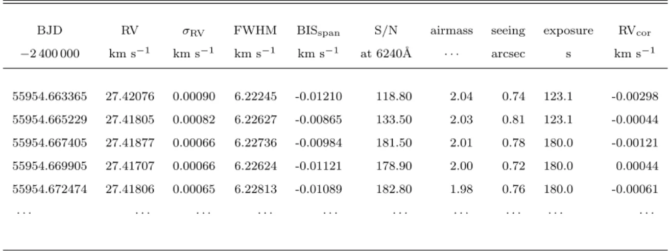
Table 1. Radial velocities of all spectra of 55 Cnc observed with HARPS and HARPS-N. The columns are: barycentric Julian date, radial velocity, radial velocity errorbars, full width at half maximum of the cross-correlation function, span in bisector slope, as defined in Queloz et al. (2000), signal- to-noise ratio at 6240 ˚A, airmass, seeing measured by the La
Silla seeing monitor, exposure time, and radial velocities with the five planet Doppler displacement removeda.
BJD RV σRV FWHM BISspan S/N airmass seeing exposure RVcor
−2 400 000 km s−1 km s−1 km s−1 km s−1 at 6240˚A · · · arcsec s km s−1 55954.663365 27.42076 0.00090 6.22245 -0.01210 118.80 2.04 0.74 123.1 -0.00298 55954.665229 27.41805 0.00082 6.22627 -0.00865 133.50 2.03 0.81 123.1 -0.00044 55954.667405 27.41877 0.00066 6.22736 -0.00984 181.50 2.01 0.78 180.0 -0.00121 55954.669905 27.41707 0.00066 6.22624 -0.01121 178.90 2.00 0.72 180.0 0.00044 55954.672474 27.41806 0.00065 6.22813 -0.01089 182.80 1.98 0.76 180.0 -0.00061 · · · ·
aThe full table is published in the journal’s electronic edition. A portion is reproduced here to show its form and
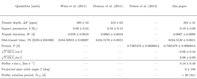
Table 2. Analysis priors and results. The quantities determined by photometry are inserted as Gaussian priors taken from three papers. The values our analysis yields are
included to illustrate that our fits did not force solutions to unrealistic values.
Quantities [units] Winn et al. (2011) Demory et al. (2011) Nelson et al. (2014) this paper
Transit depth, ∆F [ppm] 380 ± 52 410 ± 63 · · · 384 ± 41 Impact parameter, b [R?] 0.00 ± 0.24 0.16 ± 0.13 · · · 0.18 ± 0.08 Transit duration, W [d] 0.658 ± 0.0019 0.0665 ± 0.0019 · · · 0.0667 ± 0.0008 Mid-transit time, T 0 [BJD-2 450 000] 6184.50910 ± 0.00087 6184.5170 ± 0.0015 · · · 6184.5120 ± 0.0011 Period, P [d] · · · 0.7365478 ± 0.0000014 0.7365478 ± 0.0000014 √ V sin i?cos β · · · −0.06 ± 0.42 √ V sin i?sin β · · · 0.06 ± 0.69 Stellar v sin i?[km s−1] · · · 0.18 ± 0.48
Projected spin–orbit angle β [deg] · · · 0 ± 180