Interpolative and extrapolative reasoning in propositional theories using qualitative knowledge about conceptual spaces

O

pen

A

rchive

T

OULOUSE

A

rchive

O

uverte (

OATAO

)

OATAO is an open access repository that collects the work of Toulouse researchers and

makes it freely available over the web where possible.

This is an author-deposited version published in :

http://oatao.univ-toulouse.fr/

Eprints ID : 13173

To link to this article :

DOI:10.1016/j.artint.2013.07.001

URL :

http://dx.doi.org/10.1016/j.artint.2013.07.001

To cite this version :

Schockaert, Steven and Prade, Henri Interpolative and

extrapolative reasoning in propositional theories using qualitative knowledge

about conceptual spaces. (2013) Artificial Intelligence, vol. 202 . pp. 86-131.

ISSN 0004-3702

Any correspondance concerning this service should be sent to the repository

administrator:

staff-oatao@listes-diff.inp-toulouse.fr

Interpolative and extrapolative reasoning in propositional

theories using qualitative knowledge about conceptual spaces

Steven Schockaert

a

,

∗

_{, Henri Prade}

b

a_{Cardiff University, School of Computer Science & Informatics, 5 The Parade, Cardiff CF24 3AA, UK}

b_{Toulouse University, Université Paul Sabatier, IRIT, CNRS, 118 Route de Narbonne, 31062 Toulouse Cedex 09, France}

a b s t r a c t

Keywords: Commonsense reasoning Conceptual spaces Interpolative reasoning Analogical reasoning

Many logical theories are incomplete, in the sense that non-trivial conclusions about particular situations cannot be derived from them using classical deduction. In this paper, we show how the ideas of interpolation and extrapolation, which are of crucial importance in many numerical domains, can be applied in symbolic settings to alleviate this issue in the case of propositional categorization rules. Our method is based on (mainly) qualitative descriptions of how different properties are conceptually related, where we identify conceptual relations between properties with spatial relations between regions in Gärdenfors conceptual spaces. The approach is centred around the view that categorization rules can often be seen as approximations of linear (or at least monotonic) mappings between conceptual spaces. We use this assumption to justify that whenever the antecedents of a number of rules stand in a relationship that is invariant under linear (or monotonic) transformations, their consequents should also stand in that relationship. A form of interpolative and extrapolative reasoning can then be obtained by applying this idea to the relations of betweenness and parallelism respectively. After discussing these ideas at the semantic level, we introduce a number of inference rules to characterize interpolative and extrapolative reasoning at the syntactic level, and show their soundness and completeness w.r.t. the proposed semantics. Finally, we show that the considered inference problems are PSPACE-hard in general, while implementations in polynomial time are possible under some relatively mild assumptions.

1. Introduction

Symbolic approaches to knowledge representation typically start from a finite set of natural language labels, which are associated to atomic propositions (in propositional settings), to predicates (in first-order settings), or to atomic concepts (in description logics). The meaning of these labels is then expressed implicitly by encoding how the corresponding propositions are related to each other using a logical theory. Clearly, such a logical theory can only capture a small fraction of the actual meaning of the labels at the cognitive level. Formalizing commonsense reasoning then boils down to developing principled approaches to extend or refine logical inference, such that the conclusions that can be derived from a logical theory become, in some way, closer to what we infer at the cognitive level. Some approaches to non-monotonic reasoning[1], for instance, deal with exceptions by assuming that rules only apply to typical instances of the concepts involved or are only valid in

normal situations, even though these notions of typicality and normality are not explicitly expressed at the symbolic level.

Essentially, such approaches are non-monotonic because the factual knowledge they work on is incomplete: we may know

*

Corresponding author.

that Tweety is a bird, but not that it is a penguin. Later observations may enrich our factual knowledge base, necessitating a revision of some of the assumptions that were made (e.g. Tweety can fly). As another form of commonsense reasoning, in this paper we look at techniques for dealing with a lack of generic knowledge. For the ease of presentation, we will assume that generic knowledge is expressed as a set of propositional rules. We are then interested in situations where factual knowledge is, in principle, complete, but where none of the given rules applies to the situation at hand. For instance, we may know that it is advisable to rest (i) when feeling nauseated and having a high fever, and (ii) when feeling nauseated without any fever, but not have any information about what is advisable in case of nausea with a mild fever.

Similarity-based reasoning Humans can often cope with such a lack of knowledge by drawing analogies, or by resorting to

knowledge about similar situations[2,3]. This observation has led to a number of theories of approximate reasoning, which are mainly based on the premise that from similar conditions we can draw similar conclusions. Most notably, a large number of fuzzy set based approaches have been proposed that build on the idea that the more a situation is compatible with the fuzzy labels in the antecedent of a rule, the more it should be compatible with the fuzzy labels in its consequent. Such rules, called gradual rules in[4], are based on a measure of similarity that is implicit in the definition of the membership functions of the fuzzy labels. Related to gradual rules, certainty rules[4]rather encode that the more similar a situation is to the fuzzy labels in the antecedent of a rule, the more certain that the consequent holds. Some related approaches avoid the use of fuzzy sets and rather encode similarity assessments in an explicit way (e.g.[5–7]). Given that a1 and a

→

b hold,

such methods allow to derive b with a certainty that depends on the degree of similarity sim

(

a

,

a1

)

.

Despite the intuitive appeal of similarity-based approaches, and their popularity in the context of control and classi-fication problems, they face a number of difficulties when used for commonsense reasoning. First, quantitative similarity degrees can be hard to obtain in practice, a problem which is aggravated by the observation that similarity judgements are context-dependent [8,9]. The quantitative nature of similarity degrees also makes it difficult to encode rules, e.g. exactly how similar should a given premise a1 be to the antecedent of the rule a

→

b to derive b with a given certainty? Finally,

similarity based methods tend to lack a principled way of dealing with conjunctions. For instance, assume that the rule

a

∧

b

→

c and the facts a1and b1 are known to hold, and moreover sim

(

a

,

a1

) =

0

.

6 and sim

(

b

,

b1

) =

0

.

4. To assess whether

we can plausibly derive a1

∧

b1

→

c using similarity based reasoning, we would need to assess to what extent a1

∧

b1 is

similar to a

∧

b. Usually, a truth-functional approach is assumed, assuming e.g. sim

(

a

∧

b

,

a1

∧

b1

) =

min

(

sim

(

a

,

a1

),

sim

(

b

,

b1

))

or sim

(

a

∧

b

,

a1

∧

b1

) =

sim

(

a

,

a1

) ·

sim

(

b

,

b1

)

. Such views, however, are hard to justify from a cognitive point of view.

Betweenness The aforementioned shortcomings of similarity-based reasoning seem closely related to the use of degrees.

A key observation is that in practice, similarity-based approaches are often used to implement a form of interpolation of symbolic rules: given the rules a1

→

b1 and a3

→

b3, and a premise a2 which is known to be between a1 and a3,

a conclusion is obtained between b1 and b3. Interpolative inference, however, can also be implemented in a qualitative

way, taking betweenness as primitive rather than similarity. Indeed, it suffices to know which propositions are conceptually between a1and a3and which propositions are between b1 and b3. For instance, since a mild fever is conceptually between

high fever and no fever, in the earlier example we conclude that resting is advised in case of nausea with a mild fever. This basic form of interpolative inference can then be further refined, depending on the kind of background information that is available about the conceptual relationships between the propositions (labels). For example, if we know that a2 is closer to a1 than to a3, we may insist that the conclusion should also be closer to b1 than to b3. The idea of interpolating symbolic

knowledge can also be extended to various forms of extrapolative inference, as is illustrated in the following example.

Example 1. Consider the following knowledge base, containing observations about the comfort level of different housing options:

mansion

→

exclusive (1)

villa

∧

suburbs

→

luxurious (2)

apartment

∧

suburbs

→

basic (3)

apartment

∧

centre

→

very-comfortable (4)

Clearly, this knowledge base is incomplete. For instance, we have no information at all about the comfort level of a villa in the centre. However, from the rules that are provided, it seems reasonable to assume that villas are more comfortable than apartments (by comparing(2)and(3)) and that housing in the centre is more comfortable than housing in the suburbs (by comparing (3)and(4)). As a form of extrapolative inference, this leads us to conclude that a villa in the centre would at least be as comfortable as a villa in the suburbs, i.e. either luxurious or exclusive. We may also wonder about apartments in the outskirts of the city. As living in the outskirts is conceptually between living in the centre and living in the suburbs, from(3)and(4)we may reasonably assume, as a form of interpolative inference, that the comfort level of an apartment in the outskirts would be between basic and very-comfortable.

Objectives of the paper The aim of this paper is to develop a principled approach to interpolative and extrapolative reasoning,

as a general way to avoid the use of degrees when dealing with incomplete generic knowledge. In particular, we address the following research questions:

1. How can interpolative and extrapolative inference be formalized? What are its computational properties and how can automated inference procedures be implemented?

2. What is the nature of the background knowledge that is needed to support interpolative and extrapolative reasoning? 3. What is the semantic justification for interpolation and extrapolation? While most approaches to non-monotonic

rea-soning have a principled semantic foundation, typically based on the notion of preferred worlds[10,1] or the idea of stable models[11,12], this is to a much lesser extent the case for current methods that deal with incompleteness of rule bases.

The underlying idea is that among all possible refinements of a given knowledge base we favour those which are most

regular, an intuition which will be formalized using the theory of conceptual spaces[13]. This theory posits that natural language labels can be identified with a convex region in a particular geometric space — called a conceptual space — whose dimensions correspond to cognitively meaningful qualities. Using conceptual spaces, notions such as betweenness can be given a clear geometric interpretation, which allows us to derive a semantic characterization of various interpolative and extrapolative inference relations. It is important to note, however, that although conceptual spaces are crucial to justify our approach, in practical applications, we do not actually require that the conceptual space representations of properties are available. In particular, the inference mechanism itself will only require qualitative knowledge about how the conceptual representations of labels are spatially related. For instance, to support a basic interpolative inference relation, it is only required that we know which labels are conceptually between which other labels. Furthermore note that this form of commonsense reasoning will actually be monotonic: increasing the rule base may allow us to refine earlier conclusions, but will never violate them. In contrast, in the setting of non-monotonic reasoning, increasing the factual knowledge may lead us to consider different rules to be applicable, as more specific rules may override more general ones.

Depending on the considered application, the required qualitative knowledge can be provided by an expert or it can be derived automatically using data-driven techniques. In the first case, an expert may choose to manually encode some rules, and rely on interpolation or extrapolation to avoid the need for a complete specification of the considered domain (e.g. explicitly enumerating the comfort level for all housing types and all location types). The resulting inference relation would be guaranteed to provide sound conclusions, although for those parts of the domain that were not explicitly modelled by the expert, available information may be less precise (but not trivial). In the second case, where data-driven techniques are used to obtain background information about the conceptual relationship of different labels (e.g. by analysing documents from the web), the aim is rather to generate plausible conclusions from imperfect conceptual background knowledge. In this way, we can combine the rigour of a logic-based framework with the flexibility of data-driven methods. The commonsense aspect of the approach thus lies in the possibility to go beyond classical deduction by taking advantage of structural domain knowledge that has been induced from data, without resorting to purely statistical techniques as in[14].

Organization The paper is structured as follows. After discussing related work in Section2, we present a high-level overview of our approach in Section3. Section4subsequently discusses in more detail how qualitative spatial descriptions of con-ceptual spaces can be used to encode the concon-ceptual relationship of different atomic properties. Next, in Section 5 we investigate how conceptual relations between atomic properties can be leveraged to conceptual relations between unions and intersections of properties (represented as sets of vectors of properties), and how the latter conceptual relations can be used to refine a given rule base at the semantic level. In Section6we then focus on the syntactic level: we introduce a set of inference rules and show that they are sound and complete w.r.t. the semantics from Section5. Section 7analyses the computational complexity of interpolative and extrapolative reasoning and presents an implementation method. In Section8

we present some further thoughts on how to apply our method in practice, and in particular on the question of how to handle inconsistencies that are introduced by our method. We present our conclusions and a number of directions for future work in Section9. Finally, note that this paper forms a substantially extended and revised version of[15]. Among others, we now provide a complete characterization of extrapolative inference and include the idea of comparative distance (whereas only the interpolative inference relation was characterized in[15]). We moreover present an implementation method, as well as the proofs.

2. Related work

Our work is clearly related to existing approaches in cognition and knowledge representation that are based on a spatial representation of knowledge. However, our approach also touches upon several other domains, including non-monotonic reasoning, similarity-based reasoning, regularization in machine learning, and qualitative physics. We briefly clarify the relationship with each of these domains.

Spatial representations of meaning

One of the central motivations of this paper is to approach commonsense reasoning by abandoning the idea that atomic propositions are independent from each other, in favour of a view which allows them to be conceptually related in a way that cannot be fully expressed at the logical level. Although atomic propositions are traditionally assumed to be independent, several 20th century philosophers have argued against such a view. Wittgenstein[16] was among the first to realize that

sometimes we need more than a purely syntactic approach to logic, considering that atomic logical formulas may exclude each other while they are not contradictory. A statement such as place P is green at time T and place P it is blue at time T is treated as nonsensical by Wittgenstein rather than false, where he writes “It is, of course, a deficiency of our notation that it does not prevent the formation of such nonsensical constructions, and a perfect notation will have to exclude such structures by definite rules of syntax” [16]. In the same spirit, Carnap[17] uses the notion of an attribute space to group predicates of the same type. An attribute space is an abstract representation of a certain domain. For instance, the attribute space of colours consists of all (infinitely many) colour instances. In practice, these attribute spaces are usually described using a finite set of labels, which correspond to predicates at the logical level. By thus partitioning the predicates into separate attribute spaces, one can restrict interpretations to those that make exactly one predicate true from each attribute space, for any given individual. Quine[18]uses the related notion of a quality space to characterize similarity, putting forward the view that similarity cannot be defined in logical terms, and thus requires a deeper representation of atomic propositions. These works have led to the more recent development of conceptual spaces [13] by Gärdenfors, in an attempt to use the idea of a spatial representation of meaning to tackle problems in artificial intelligence (AI), among others. Conceptual spaces will be discussed in more detail in Section4.

Apart from the work on conceptual spaces, the idea of assuming a spatial representation to reason about concepts also underlies [19], where an approach to integrate heterogeneous databases is proposed based on spatial relations between concepts. This approach starts from the observation that types from one database may not have an exact counterpart in another database. Conceptual relations between types are therefore considered which express e.g. that all typical instances of type A belong to type B but some instances of type A may be outside B. Such relations can formally be modelled as egg/yolk relations, which are a form of qualitative spatial relations between ill-defined spatial regions. Somewhat related, in

[20] we presented a general method for merging conflicting propositional knowledge bases coming from different sources, based on the view that different sources may have a slightly different understanding of a given label. The different ways in which such a label may be understood are encoded in terms of four primitive relations that essentially correspond to qualitative spatial relations between (unknown) geometric representations of the labels. Although the kind of spatial relations encountered in these existing works are mainly mereotopological, qualitative spatial reasoning about betweenness is an active topic of research[21,22].

Non-monotonic reasoning

In general, several facets of commonsense reasoning have been extensively studied within the field of AI. Of particular interest is the work on System P for reasoning about rules with exceptions[1]. In this approach, a non-monotonic conse-quence relation is defined by encoding axiomatically how new rules may be derived from existing rules. In particular, the non-monotonic consequence relation

|∼

is defined by the following inference rules:

Reflexivity

α

|∼

α

Left logical equivalence If

α

≡

α

′ _and

_α

_|∼β

_then

_α

′

_|∼β

Right weakening If

β |H β

′and

α

|∼ β

then

α

|∼β

′

OR If

α

|∼

γ

and

β|∼

γ

then

α

∨ β|∼

γ

Cautious monotony If

α

|∼β

and

α

|∼

γ

then

α

∧ β|∼

γ

Cut If

α

∧ β|∼

γ

and

α

|∼β

then

α

|∼

γ

where

≡

and

|H

denote equivalence and entailment in classical logic, respectively. Intuitively,

α

|∼β

means that in normal situations where

α

holds, it is also the case that

β

holds. The normative approach by System P about how a non-monotonic consequence relation should behave has been very influential in the field of non-monotonic reasoning. While the purpose of our paper is not to study non-monotonic consequence relations, our approach does resemble System P in that our goal is also to produce new rules, which are appropriate to a given situation. However, whereas System P is concerned with finding the most specific rules that are compatible with our (incomplete) knowledge about the situation at hand, in interpolative and extrapolative reasoning there is no genuine issue of incompleteness at the factual level. Rather, we are interested in situations where the given situation is not explicitly covered by a rule base, but is intermediate between, or analogous to situations that are covered.

Similarity-based reasoning

Somewhat related, several authors have studied similarity-based consequence relations which are based on the intu-ition that

α

approximately entails

β

iff every model of

α

is similar to some model of

β

[23,6,24]. In[25], for instance, a based consequence relation is contrasted with the consequence relation from System P, revealing that similarity-based reasoning satisfies monotonicity and most of the axioms of System P, but not the cut rule. More generally, a large number of authors have proposed systems for approximate, similarity-based reasoning within the field of fuzzy set theory. Most of these works are based on Zadeh’s generalized modus ponens[26] (but see [27] for an early example of a more qualitative approach), which allows us to derive a fuzzy restriction on the value of variable Y from the knowledge that if

X is A then Y is B and X is A′_{with A, A}′ _{and B fuzzy sets. The basic idea is that the more A is similar to A}′_{, the more}

the inferred restriction on Y will be close to B. When this idea is applied to a set of parallel rules, such that the fuzzy sets in the antecedents of the rules overlap, it leads to a form of interpolative reasoning. Furthermore, several authors have

proposed methods to interpolate fuzzy rule bases in general, i.e. without requiring overlap of the fuzzy sets; we refer to

[28] for a recent overview. While these techniques are also about interpolating rules, they differ from our approach in a number of ways. First, they are mostly restricted to uni-dimensional, numerical domains, and they require that quantitative representations of symbolic labels be available in the form of fuzzy sets. Furthermore, they treat logical connectives, such as conjunctions in the antecedent, in a truth-functional (and therefore heuristic) way.

In [29], a logic called CSL is introduced which has a construct A

⇔

B denoting all objects that are more similar to

instances of concept A than to instances of concept B. The qualitative nature of this logic brings it closer to the approach we present in this paper. As it is based exclusively on closeness, and not on other aspects of spatial localization such as being in between, CSL is not directly suitable as a basis for interpolative or extrapolative reasoning. Interestingly, however, as a result of this restriction, CSL can be described using a preferential semantics[30].

Regularity

In the propositional setting, the idea of interpolation and extrapolation has been studied in [31], but from a rather different angle. In particular, the paper discusses how the belief that certain propositions hold at certain moments in time can be extended to beliefs about other moments in time, using persistence assumptions as a starting point. Nonetheless, as in our paper, the main idea is to use general meta-principles to find those completion(s) of a knowledge base that are most regular in some sense.

The idea of regularity can also be found in work on analogical proportions. An analogical proportion is an expression of the form a

:

b

::

c

:

d which reads as a is to b as c is to d. If a, b, c and d are binary propositions, this can be formalized

as

(

a

→

b

≡

c

→

d

) ∧ (

b

→

a

≡

d

→

c

)

(see [32]). In [33], an approach to classification is outlined which uses the view that, as a form of regularity, the more of the condition attributes of three training items form an analogical proportion with the condition attributes of the item to be classified, the more it becomes likely that also the decision attribute should form an analogical proportion. Using connectives from multi-valued logic, analogical proportions can be defined for graded propositions, which allows us to extend this idea to numerical attributes. In[34], an extrapolative inference mechanism has been proposed which is based on such analogical proportions between graded proportions. The latter technique can be seen as a special case of the approach we develop in this paper. In this paper, however, we also consider forms of interpolative and extrapolative reasoning that are not based on analogical proportions, and the proposed techniques are moreover not restricted to linearly ordered domains.

More generally, the idea of regularity appears in various forms in learning settings. In graph regularization[35], for in-stance, the desire for regularity is even made explicit in the form of a graph which connects instances that should receive a similar classification. In other approaches, the idea of regularity is implicit in the choice of the underlying classification functions that are allowed (e.g. being restricted to hyperplanes in the case of support vector machines), and is thus imposed to avoid overfitting. As an example of another domain where the idea of regularity surfaces,[36] presents an approach to derive a preference ordering, starting from a set of generic preferences. To choose a specific ordering among all those sat-isfying the constraints, the principle of minimal specificity from possibility theory is adopted as a way to avoid introducing any irregularities that have not been explicitly specified as constraints.

The notion of matrix abduction, proposed in[37] is also related to our work in its use of regularity as a criterion to complete missing values, although it operates at a lower-level representation. Specifically, consider a matrix whose rows correspond to objects and whose columns correspond to binary features, such that exactly one entry of the matrix is ‘?’, corresponding to a missing value, and all the other entries are 0 or 1. Then[37]proposes to choose the missing value such that the regularity of the matrix is maximized. Specifically, a partial order relation is induced from both of the possible completions of the matrix, and the completion which is favoured is the one whose associated partial order relation is most natural in some sense. Note that, somewhat related, in abductive reasoning for causal diagnosis, it is also common to favour the simplest explanations (e.g. preferring single fault diagnoses to explain observed symptoms).

Qualitative physics

Finally, there is some resemblance between the inference procedure presented in this paper and the early work on qualitative reasoning about physical systems[38,39], which deals with monotonicity constraints such as “if the value of x increases, then (all things being equal) the value of y decreases”. Our inference procedure differs from these approaches as the domains we reason about do not need to be linearly ordered. Moreover, in the special case of linearly ordered domains, we assume no prior information about which partial mappings are increasing and which are decreasing.

3. Overview of the approach

In this section, we introduce some notations and basic concepts that will be used throughout the paper. We also present the main intuitions of our approach at an informal level.

Let A1

, . . . ,

An be finite sets of labels, where each set Aicorresponds to a certain type of properties1 (e.g. colours), and the labels of Aicorrespond to particular properties of the corresponding type (e.g. red, green, orange). The labels in Ai are

assumed to correspond to jointly exhaustive and pairwise disjoint (JEPD) properties. Note that each element

(

a1

, . . . ,

an

)

from the Cartesian product

A =

A1

× · · · ×

An then corresponds to a maximally descriptive specification of the properties that some object or situation may satisfy. We furthermore assume that Ai

∩

Aj

= ∅

for i

6=

j. We will refer to the sets Aias attribute domains, and to their elements as attributes or, when used in a propositional language, as atoms.

We consider propositional rules of the form

β →

γ

, where

β

and

γ

are propositional formulas, built in the usual way from the set of atoms A1

∪ · · · ∪

An and the connectives

∧

and

∨

. Note that we do not need to explicitly consider nega-tion, as the negation of an atom a

∈

Ai corresponds to the disjunction of the atoms in Ai

\ {

a

}

. We say that an element

(

a1

, . . . ,

an

) ∈ A

is a model of a formula (or a rule)

α

, written

(

a1

, . . . ,

an

) |H

A

α

if the corresponding propositional

inter-pretation

{

a1

, . . . ,

an

}

is a model of

α

in the usual sense, where we see propositional interpretations as sets containing all atoms that are interpreted as true. For formulas (or rules or sets of rules)

α

1 and

α

2, we say that

α

1 entails

α

2,

writ-ten

α

1

|H

A

α

2 if for every

ω

∈ A

,

ω

|H

A

α

1 implies

ω

|H

A

α

2. Note that the notion of entailment we consider is classical

entailment, modulo the assumption that the propositions in each set Aiare JEPD.

Example 2. Considerthe following attribute domains:

A1

= {

row-house1

,

semi-detached1

,

bungalow

,

villa

,

mansion

,

bedsit

,

studio

,

one-bed-ap

,

two-bed-ap

,

three-bed-ap

,

loft

,

penthouse

}

A2

= {

row-house2

,

semi-detached2

,

detached

,

apartment

}

A3

= {

very-small

,

small

,

medium

,

large

,

very-large

}

A4

= {

basic

,

comfortable

,

very-comfortable

,

luxurious

,

exclusive

}

where A1 lists the housing types that are possible in the given context, A2provides a coarser description of some of these

housing types, and A3 and A4 contain the labels that are used to describe housing sizes and comfort levels respectively.

Note that subscripts are used for the housing options row-house and semi-detached to ensure that different attribute domains are disjoint. When there is no cause for confusion, we will omit these subscripts. The following set of rules R provides a partial specification of how these attribute domains are related to each other:

bungalow

→

medium bungalow

→

detached (5)

mansion

→

very-large mansion

→

detached (6)

large

∧

detached

→

lux large

∧

row-house

→

comf (7)

small

∧

detached

→

bas

∨

comf mansion

→

excl (8)

where some labels are abbreviated for the ease of presentation. For example

(

villa

,

detached

,

large

,

lux

)

is a model of each of these rules. Note that the only conclusions that can be derived from R are more or less trivial, e.g.

R

|H

Avilla

→

very-small

∨

small

∨

medium

∨

large

∨

very-large (9)

R

|H

A

(

small

∨

large

) ∧

detached

→

basic

∨

comfortable

∨

luxurious (10)

Note that(9)follows from our assumption that the labels in an attribute domain are exhaustive.

3.1. Commonsense inference

A rule base R over the atoms in

A

usually only provides an incomplete specification of how the given attribute domains are related to each other. We are interested in refining the available knowledge in R using a number of generic meta-principles. To this end, we will make use of background knowledge about the conceptual relationship of different formulas, which we assume to be encoded in a set of assertions

Σ

(to be formalized in Section6). We are then interested in defining a consequence relation

⊢

that extends the entailment relation

|H

A(i.e. supraclassicality). Specifically, we assume that the

following inference rule is valid:

R

|H

A

β →

γ

(

R

, Σ )

⊢

β →

γ

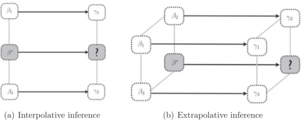
(S)

The first meta-principle we consider is that intermediate conditions should lead to intermediate conclusions.

For instance, given that both large and small detached houses have a comfort level that is between basic and luxurious, we derive that also medium detached houses should have a comfort level between these bounds. More generally, if a propositional formula

β

is conceptually between the formulas

β

1 and

β

2, the idea of interpolative inference is that whatever

we can derive from

β

should be conceptually between what we can derive from

β

1 and what we can derive from

β

2. The

Fig. 1. Modelling betweenness and parallelism between regions.

between

β

1 and

β

2 if

β

has all the features that

β

1 and

β

2 have in common. We could say, for instance, that a bistro is

conceptually between a bar and a restaurant, or that a studio is conceptually between a bedsit and an apartment. In ecology, we may consider that taiga is between tundra and temperate-forest. We could take the view that the painting style of Renoir is conceptually between the painting styles of Monet and Manet.

To encode information about betweenness at the syntactic level, we use a modality

✶

, i.e. the formula

β

1

✶

β

2 is true

whenever a situation holds which is conceptually between a situation satisfying

β

1 and a situation satisfying

β

2 (or

al-ternatively, when talking about concepts,

β

1

✶

β

2 is true for instances that are between

β

1 and

β

2). Typically, it will not

be possible to have a precise definition of

β

1

✶

β

2, as, in fact, our logical language may not be rich enough to precisely

capture exactly those situations. However, in practice, we may obtain knowledge about upper and lower approximations of

β

1

✶

β

2. We write

Σ ⊢

γ

→ β

1

✶

β

2 to denote that everything which satisfies

γ

is conceptually between

β

1 and

β

2, and

Σ ⊢ β

1

✶

β

2

→

γ

to denote that anything which is conceptually between

β

1 and

β

2should definitely satisfy

γ

.

Example 3. It is not the case that all lofts are conceptually between a three-bedroom apartment and a penthouse (e.g. a small loft with only one bedroom), so loft

→

three-bed-ap

✶

penthouse does not hold. However, we do have trivially that

three-bed-ap

∨

penthouse

→

three-bed-ap

✶

penthouse

Conversely, however, some lofts are between a three-bedroom apartment and a penthouse, so we cannot remove the dis-junct loft in the consequent of the following implication

three-bed-ap

✶

penthouse

→

three-bed-ap

∨

loft

∨

penthouse

Note that in the considered domain, there are no apartments with more than three bedrooms (with the possible exception of penthouses), hence three-bed-ap, loft and penthouse exhaustively cover all situations that are between a three-bedroom apartment and a penthouse.

On the other hand, we may consider that all studios are between bedsits and one-bedroom apartments. Under this view, we should be able to derive the following rules from

Σ

:

bedsit

∨

studio

∨

one-bed-ap

→

bedsit

✶

one-bed-ap bedsit

✶

one-bed-ap

→

bedsit

∨

studio

∨

one-bed-ap

Using the binary modality

✶

, we can define the following interpolative inference rule:

(

R

, Σ ) ⊢ β

1

→

γ

1

(

R

, Σ ) ⊢ β

2

→

γ

2

Σ ⊢ β

∗

→ β

1

✶

β

2

Σ ⊢

γ

1

✶

γ

2

→

γ

∗

(

R

, Σ ) ⊢ β

∗

→

γ

∗ (I)

A diagrammatic representation of this interpolation principle is shown inFig. 1(a): given two rules

β

1

→

γ

1 and

β

2

→

γ

2,

we derive a rule which applies to a situation

β

∗ which is intermediate between

β

1 and

β

2. The conclusion

γ

∗ of that rule

is required to exhaustively cover all situations that are intermediate between

γ

1 and

γ

2.

The second meta-principle states that analogous changes in the condition of a rule should lead to analogous changes in the conclu-sion.

Let us write

hβ

1

, β

2

i

to denote the change that is needed to convert a specification compatible with

β

1 into a

this notion of direction is not symmetric, e.g. while

h

two-bed-ap

,

three-bed-ap

i

denotes the direction of an increasing num-ber of bedrooms,

h

three-bed-ap

,

two-bed-ap

i

denotes a decreasing number. Given a third formula

β

3, we are then interested

in those situations that can be obtained by changing a situation compatible with

β

3 in the direction specified by

hβ

1

, β

2

i

.

In particular, we will write

β

3

✄

hβ

1

, β

2

i

for the formula that covers all such situations. For example, we could consider

that progressive rock differs from hard rock by having less standard song structures and arrangements, while keeping the same instruments. Then heavy-metal

✄

h

hard-rock

,

prog-rock

i

would cover all music genres that use heavy metal instruments and timbres, but less standard song structures and arrangements. This would include all progressive metal, as well as some instances of avant-garde metal, among others. In biology, we may consider that the difference between dog to coyote is analogous to the difference between cat and leopard, or to the difference between cat and lynx, which we could encode as

coyote

→

dog

✄

h

cat

,

leopard

i

and coyote

→

dog

✄

h

cat

,

lynx

i

respectively. Note in particular that we do not take into account the amount of change: while we may consider that the change from cat to leopard is bigger than the change from dog to

coyote, the direction of change is the same.

As for betweenness, we will mainly be interested in approximating

β

3

✄

hβ

1

, β

2

i

rather than finding an exact definition,

i.e. we will be looking for propositional formulas that imply, and that are implied by

β

3

✄

hβ

1

, β

2

i

.

Example 4. The change from a bedsit to a studio essentially corresponds to an increase in size and comfort. In this sense, such a change is similar to the change from a two-bedroom apartment to a three-bedroom apartment, or even to a pent-house. We may consider, for instance:

Σ ⊢

two-bed-ap

∨

three-bed-ap

∨

penthouse

→

two-bed-ap

✄

h

bedsit

,

studio

i

Σ ⊢

two-bed-ap

✄

h

bedsit

,

studio

i →

two-bed-ap

∨

three-bed-ap

∨

loft

∨

penthouse

Only the direction of the change is taken into account here, and not the amount of change. For instance, we might have

Σ ⊢

one-bed-ap

∨

two-bed-ap

∨

three-bed-ap

∨

penthouse

→

one-bed-ap

✄

h

one-bed-ap

,

two-bed-ap

i

Note that the meaning of

h. , .i

by itself cannot be expressed at the syntactic level, i.e.

. ✄ h. , .i

is treated as a ternary modality. Extrapolative inference can then be formalized as follows:

(

R

, Σ ) ⊢ β

1

→

γ

1

(

R

, Σ ) ⊢ β

2

→

γ

2

(

R

, Σ ) ⊢ β

3

→

γ

3

Σ ⊢ β

∗

→ β

1

✄

hβ

2

, β

3

i

Σ ⊢

γ

1

✄

h

γ

2

,

γ

3

i →

γ

∗

(

R

, Σ ) ⊢ β

∗

→

γ

∗ (E)

A diagrammatic representation is given inFig. 1(b). In this case, three rules

β

1

→

γ

1,

β

2

→

γ

2 and

β

3

→

γ

3 are available,

and we are interested in deriving conclusions about a fourth situation

β

∗_{which differs from}

_β

1 as

β

3 differs from

β

2. The

conclusion

γ

∗_{which is derived exhaustively covers all situations that differ from}

_γ

1 as

γ

3 differs from

γ

2.

Finally, we assume that the consequence relation

⊢

is deductively closed:

(

R

, Σ )

⊢

β

1

→

γ

1

(

R

, Σ )

⊢

β

2

→

γ

2

{β

1

→

γ

1

, β

2

→

γ

2

} |H

A

β

3

→

γ

3

(

R

, Σ )

⊢

β

3

→

γ

3

(D)

Example 5. Consider the rules fromExample 2. Applying (S), we immediately have

(

R

, Σ ) ⊢

bungalow

→

medium

(

R

, Σ ) ⊢

mansion

→

very-large

Assuming

Σ ⊢

bungalow

∨

villa

∨

mansion

→

bungalow

✶

mansion

Σ ⊢

medium

✶

very-large

→

medium

∨

large

∨

very-large we find using (I) that

(

R

, Σ ) ⊢

bungalow

∨

villa

∨

mansion

→

medium

∨

large

∨

very-large

and using (D) that

(

R

, Σ ) ⊢

villa

→

medium

∨

large

∨

very-large which refines the trivial conclusion that we obtained in

(

R

, Σ ) ⊢

large

∧

detached

→

lux

(

R

, Σ ) ⊢

large

∧

row-house

→

comf

(

R

, Σ ) ⊢

small

∧

detached

→

bas

∨

comf

If we now assume that (writing det for detached)

Σ ⊢ (

large

∨

medium

∨

small

∨

very-small

) ∧

row-house

→ (

large

∧

row-house

) ✄ h

large

∧

det

,

small

∧

det

i

Σ ⊢

comf

✄

h

lux

,

bas

∨

comf

i →

bas

∨

comf

then (E) yields

(

R

, Σ ) ⊢ (

large

∨

medium

∨

small

∨

very-small

) ∧

row-house

→

bas

∨

comf (11)

from which we obtain using (D) that

(

R

, Σ ) ⊢

medium

∧

row-house

→

bas

∨

comf . Indeed, the rule in(11)plays the role of

β

1

→

γ

1from the definition of (D), whereas the rule

β

2

→

γ

2 is trivial.

At this point it may not be clear whether the inference relation defined by (S), (I), (E) and (D) always behaves according to intuition, nor what the implications are at the semantic level of adopting (I) and (E). To this end, in the following sections, we will develop a semantic counterpart of the inference relation

⊢

, which will clarify the nature of the modalities

✶

and

✄

h,i

and will allow us to implement decision procedures for reasoning tasks of interest. A crucial issue that will be discussed in detail is the interaction between the aforementioned modalities on the one hand, and logical conjunction on the other hand, e.g. discussing under which conditions

(

α

1

∧ β

1

) ✶ (

α

2

∧ β

2

)

is equivalent to

(

α

1

✶

α

2

) ∧ (β

1

✶

β

2

)

.

The principles (I) and (E) allow us to refine a rule base R by exploiting background knowledge about the conceptual relationship of labels from the same attribute domain. This background knowledge is of a qualitative nature. Extrapolative reasoning, for instance, is based on the idea of direction of change, but does not take the amount of change into account. An analogical proportion such as a

:

b

::

c

:

d, on the other hand, not only expresses that the change from a to b goes in

the same direction as the change from c to d, but also that the amount of change between a and b is the same as the amount of change between c and d[40]. To take information about the amount of change into account, and thus generalize analogical reasoning — making it also more cautious when necessary — we will use expressions such as

β

1

✄

[λ,µ]

hβ

2

, β

3

i

where 0

6

λ 6

µ

< +∞

. Intuitively, this formula covers all situations that can be obtained by changing

β

1 in the same

direction as the change from

β

2 to

β

3, such that the amount of change is between

λ

and

µ

times as large as the amount of

change between

β

2 and

β

3. This allows us to make inferences which are more precise in cases where suitable information

about the amount of change is available. For example, knowing that the amount of change between dog and coyote is approximately the same as the amount of change between cat and lynx, the latter relationship is more useful than the relationship between cat and leopard if we want to derive knowledge about coyotes from knowledge about dogs.

The most straightforward use of this generalization is to express whether the amount of change from

β

1 should be

smaller, equal, or larger than the amount of change from

β

2to

β

3. In particular,

β

1

✄

[1,1]

hβ

2

, β

3

i

corresponds to the solution X that makes

β

1

:

X

:: β

2

: β

3a perfect analogical proportion, while

β

1

✄

[0,1[

hβ

2

, β

3

i

and

β

1

✄

]1,+∞[

hβ

2

, β

3

i

express amounts

of change that are smaller and larger, respectively, than the amount of change from

β

2 to

β

3. Note that

β

1

✄

[0,+∞[

hβ

2

, β

3

i

corresponds to

β

1

✄

hβ

2

, β

3

i

. Also note that in the aforementioned cases, the approach remains entirely qualitative. Other

choices for the intervals

[λ,

µ

]

may give the approach a more numerical flavour, and would mainly be useful in scenarios where the conceptual relationships are obtained using data-driven techniques.

For

τ

a non-empty subset of

[

0

, +∞[

, Principle (E) can be refined to

(

R

, Σ ) ⊢ β

1

→

γ

1

(

R

, Σ ) ⊢ β

2

→

γ

2

(

R

, Σ ) ⊢ β

3

→

γ

3

Σ ⊢ β

∗

→ β

1

✄

τ

hβ

2

, β

3

i

Σ ⊢

γ

1

✄

τ

h

γ

2

,

γ

3

i →

γ

∗

(

R

, Σ ) ⊢ β

∗

→

γ

∗ (E’)

Along similar lines, for

σ

a non-empty subset of

[

0

,

1

]

, we consider expressions of the form

β

1

✶

σ

β

2to put constraints on

the relative closeness to

β

1 and

β

2. Specifically,

β

1

✶

[0,0.5[

β

2 corresponds to those situations between

β

1 and

β

2 that

are closer to

β

1 than to

β

2. Note that

β

1

✶

[0,0.5[

β

2 is a refinement of the construct

β

1

⇔

β

2 from CSL [29], as

be-tweenness is not required in CSL, only comparative closeness. Similarly,

β

1

✶

]0.5,1]

β

2 corresponds to situations that are

closer to

β

2 than to

β

1, and

β

1

✶

[0.5,0.5]

β

2 to situations that are exactly halfway. When data-driven techniques are used,

other intervals may again be useful. In scenarios where labels can be assumed to be equidistant, we may also know e.g. that small

→

very-small

✶

_[0.25,0.25]very-large and large

→

very-small

✶

_[0.75,0.75]very-large, where the idea is that medium is

Principle (I) can be refined to

(

R

, Σ ) ⊢ β

1

→

γ

1

(

R

, Σ ) ⊢ β

2

→

γ

2

Σ ⊢ β

∗

_{→ β}

1

✶

σ

β

2

Σ ⊢

γ

1

✶

σ

γ

2

→

γ

∗

(

R

, Σ ) ⊢ β

∗

→

γ

∗ (I’)

Example 6. Consider again the setting ofExample 5, and assume that a villa is conceptually halfway between a bungalow and a mansion, and that a large house is conceptually halfway between a medium house and a very-large house. We then get

Σ ⊢

villa

→

bungalow

✶

_[0.5,0.5]mansion (12)

Σ ⊢

medium

✶

_[0.5,0.5]very-large

→

large (13)

which allows us the obtain the refined conclusion

(

R

, Σ ) ⊢

villa

→

large using (I’) and (D). Alternatively, we could assume

that a villa is conceptually closer to a bungalow than to a mansion, by assuming that

Σ ⊢

bungalow

∨

villa

→

bungalow

✶

_[0,0.5[mansion Together with

Σ ⊢

medium

✶

_[0,0.5[very-large

→

medium

∨

large we would then find R

⊢

villa

→

medium

∨

large.

3.2. Mappings between attribute domains

At the semantic level, a rule base R can be seen as a mapping between sets of vectors of attributes. In particular, assume that all the labels in the antecedents of the rules in R belong to the attribute domains B1

, . . . ,

Bs and that the labels in the consequents belong to C1

, . . . ,

Ck. The rule base R can then equivalently be expressed as a function fR from subsets of

B =

B1

× · · · ×

Bsto subsets of

C =

C1

× · · · ×

Ck, defined for X

⊆ B

as

fR

(

X

) =

\

(

Y

∈

2C

¯

¯

¯

R

|H

A

Ã

_

(x1,...,xs)∈X s

^

i=1 xi

!

→

Ã

_

(y1,...,yk)∈Y k

^

i=1 yi

!)

where

A =

A1

× · · · ×

An and

{

A1

, . . . ,

An

} = {

B1

, . . . ,

Bs

} ∪ {

C1

, . . . ,

Ck

}

as before. It is not hard to see that this function indeed expresses the same knowledge as the rule base R. Furthermore, there exists a single Y∗

_∈

₂C

such that fR

(

X

) =

Y∗ and R

|H

A

Ã

_

(x1,...,xs)∈X s

^

i=1 xi

!

→

Ã

_

(y1,...,yk)∈Y∗ k

^

i=1 yi

!

Example 7. Consider again the rules base fromExample 2. We have that

B =

A1

×

A2

×

A3, as no rule refers to comfort

levels in its antecedent, and

C =

A2

×

A3

×

A4, as only the coarser housing types of A2 are referred to in the consequent of

rules. We find that a small detached villa is either basic or comfortable:

fR

¡©

(

villa

,

det

,

small

)

ª¢

=

©

(

det

,

small

,

bas

), (

det

,

small

,

comf

)

ª

Indeed, from

small

∧

detached

→

bas

∨

comf It follows that

small

∧

detached

∧

villa

→ (

bas

∨

comf

) ∧

small

∧

detached from which we can already conclude

fR

¡©

(

villa

,

det

,

small

)

ª¢

⊆

©

(

det

,

small

,

bas

), (

det

,

small

,

comf

)

ª

It is furthermore clear that there are no rules in R which could be used to further refine fR

({(

villa

,

det

,

small

)})

.

Similarly, we find that a bungalow is detached and medium-sized, while we find no restrictions on the possible comfort levels: fR

¡©

(

bun

,

x

,

y

)

¯

¯,

x

∈

A2

,

y

∈

A3

ª¢

=

©

(

det

,

medium

,

z

)

¯

¯

z

∈

A4

ª

We may see fR as an approximate (i.e. incomplete) model of a given domain, which may be refined as soon as new information becomes available. In particular, for two 2B

→

2C functions f and f′ _{which are monotone w.r.t. set inclusion,}

we say that f is a refinement of f′_{, written f}

₆

_f′_{, iff}

∀

X

⊆

B

_.

_f

₍

_X

_{) ⊆}

_f′

₍

_X

₎

₍₁₄₎

This idea of using monotone set-valued functions to describe approximate models is closely linked to the theory of Scott domains; see e.g.[41]for an elaboration of this idea. At the semantic level, completing the rule base R boils down to refin-ing the correspondrefin-ing function fR. In our approach, such refinements will be based on meta-knowledge about the nature of the relationship between

B

and

C

. This will lead us to replace fR by the largest refinement, w.r.t.

6

, which is compatible with the imposed meta-knowledge. In particular, as will become clear below, Principles (I) and (E) amount to refine fR by imposing some form of monotonicity, whereas (I’) and (E’) amount to refine fR by imposing a form of linearity. As could be expected, the meta-knowledge underlying (I’) and (E’) is stronger than the meta-knowledge underlying (I) and (E).

4. Formalization using conceptual spaces

The approach sketched in Section3requires information about how the labels of an attribute domain are conceptually related to each other. Provided that this information is available, inference can be carried out purely at the symbolic level. However, to justify the inference procedure, and to provide an adequate semantics for it, we need to be precise on how relationships such as betweenness should be interpreted. To this end, we assume that the cognitive meaning of the attributes can be represented geometrically, as convex regions in a conceptual space. Conceptual relationships can then be given a clear spatial interpretation, as will be discussed in Section4.1. Taking advantage of this link with conceptual spaces, Section4.2

subsequently reviews some opportunities for the acquisition of conceptual relations. Finally, Section4.3presents the idea of regular mappings between conceptual spaces as a basis for interpolative and extrapolative reasoning.

4.1. Geometric modelling of attribute domains

The theory of conceptual spaces [13] is centred around the assumption that the meaning of a natural property can be adequately modelled as a convex region in some geometric space. Formally, a conceptual space is the Cartesian product

Q1

×· · ·×

Qmof quality dimensions, each of which corresponds to an atomic, cognitively meaningful feature, called a quality. A standard example is the conceptual space of colours, which can be described using the quality dimensions hue, saturation and intensity. Labels to describe colours, in some natural language, are then posited to correspond to convex regions in this conceptual space, a view which is closely related to the ideas of prototype theory[42]. The label red for instance will be represented by the set of points whose hue is in the spectrum normally associated with red, whose saturation is sufficiently high, and whose intensity is neither too high nor too low. Note that while e.g. red may be an atomic property at the symbolic level, at the cognitive level it is defined in terms of more primitive notions. Quality dimensions may be continuous or discrete, and can even be finite. In practice, however, it is common to identify conceptual spaces with Euclidean spaces

[42], and to define cognitive similarity in terms of Euclidean distance. We will also adopt this simplifying view throughout the paper, although part of the discussion readily generalizes to more general spaces.2

Now consider again the example of housing types. A conceptual space to represent housing types would have a large number of dimensions, relating to shape, size, colour, texture, etc. Each house that exists in the world will correspond to one specific point in this conceptual space. Conversely, however, there may be points in that conceptual space which do not correspond to structures that can be physically realized, or that would not be recognized as houses (e.g. a building structure of 20 km long and 1 cm wide). Each attribute from the domain A1 corresponds to a convex region in the conceptual space,

where intuitively, e.g. the region corresponding to villa corresponds to those building structures that are more similar to prototypical villas than to prototypical instances of the other attributes in A1.

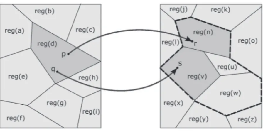
In general, each attribute domain Aithus corresponds to a partition of some conceptual space in convex regions, where each attribute of Ai corresponds to a partition class. As some regions of conceptual spaces may correspond to types of instances that do not exist in the real world, the number of partition classes may, in principle be higher than the number of attributes in Ai. We write reg

(

x

)

to denote the convex region that corresponds to label x. For example, reg

(

three-bed-ap

)

represents all sections of building structures that could be classified as three-bedroom apartments. This set will contain both points that correspond to actual apartments (which exist somewhere in the world) and possible apartments (which may in principle be built one day).

This conceptual space representation of the attributes is considerably richer than what can be described at the symbolic level, and therefore also allows for richer forms of inference. However, in most application domains, it is not reasonable to assume that such representations are available. Moreover, the precise representation of a property in a conceptual space strongly depends on the considered context and may be subjective. Usually, however, it is assumed that a particular concep-tual space representation can be obtained from a generic representation by appropriately rescaling the quality dimensions

2 _{In particular, interpolative reasoning can be carried out w.r.t. any space for which betweenness can meaningfully be defined. See e.g.[43]for a} formal-ization of conceptual spaces in terms of a primitive betweenness relation.

Fig. 2. Modelling betweenness and parallelism between regions.

[44]. Note that this observation implies that also similarity judgements may differ across contexts and people, as rescaling the dimensions may influence the relative Euclidean distance between points. For instance, while apples are usually consid-ered to be closer to tomatoes than to chocolate, in the context of desserts, they may be closer to chocolate (e.g. because both can be used in cakes). To alleviate these issues, we will rely on (mainly) qualitative knowledge about the spatial relation-ship of different properties. Such qualitative knowledge may be easier to obtain, and because the spatial relations that will be considered are invariant under affine transformations (such as rescaling the quality dimensions), they are more robust against changes in context and person. In particular, such relations are not affected by rescaling of the quality dimensions, although they would still depend on context changes that introduce additional quality dimensions.

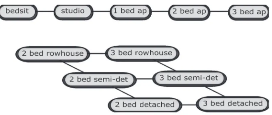
For each attribute domain Ai, we assume that information is available about betweenness and parallelism of the concep-tual space representation of its attributes. For example, we may intuitively think of a studio to be between a bedsit and a

one-bedroom apartment. In the domain of music genres, we may consider that the change from hard-rock to progressive-rock

is parallel to the change from heavy-metal to progressive-metal, and that progressive-rock is between hard-rock and

avant-garde. The notions of betweenness and parallelism are straightforwardly defined for points in Euclidean spaces. In particular,

let us write bet

(

p

,

q

,

r

)

to denote that q lies between p and r (on the same line), and par

(

p

,

q

,

r

,

s

)

to denote that the vec-tors−pq and−→ →−rs point in the same direction. The fact that point q is between points p and r means that for every point x it

holds that d

(

q

,

x

) 6

max

(

d

(

p

,

x

),

d

(

r

,

x

))

, and in particular, that whenever p and r are close to a prototype of some concept, then q is close to it as well. In this sense, we may see bet

(

p

,

q

,

r

)

as a way to express that whatever natural properties p and r have in common, p and q have them in common as well (identifying points in a conceptual space with instances). On the other hand, par

(

p

,

q

,

r

,

s

)

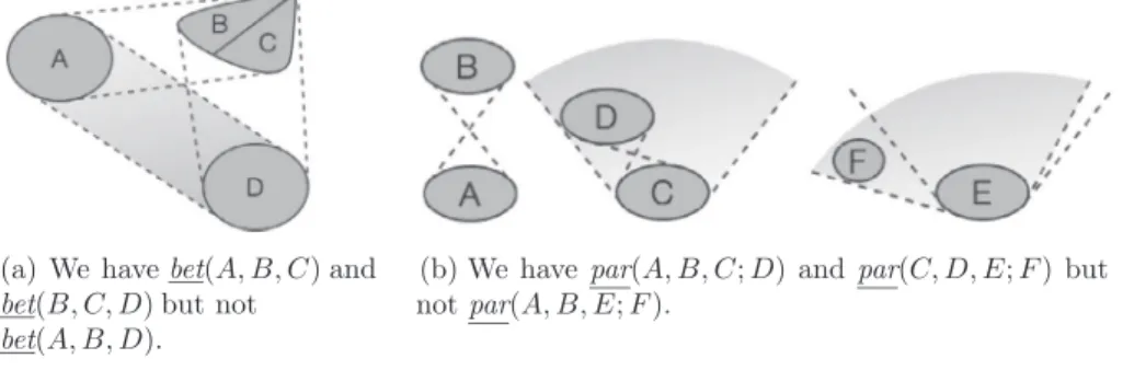
intuitively means that to arrive at s, r needs to be changed in the same way as p needs to be changed to arrive at q, i.e. at the qualitative level, p is to q as r is to s (although the amount of change may be different).

The notions of betweenness and parallelism, which are defined for points, need to be extended to regions, in order to describe relationships between attributes. As is well known, this can be done in different ways[45]. We will consider the following two notions of betweenness for regions A, B, and C (in a given Euclidean space):

bet

(

A

,

B

,

C

)

iff

∃

q

∈

B

.∃

p

∈

A

.∃

r

∈

C

.

bet

(

p

,

q

,

r

)

(15) bet

(

A

,

B

,

C

)

iff

∀

q

∈

B

.∃

p

∈

A

.∃

r

∈

C

.

bet

(

p

,

q

,

r

)

(16) In particular, if A and C are convex regions, bet

(

A

,

B

,

C

)

holds if B overlaps with the convex hull of A

∪

C , whereas bet

(

A

,

B

,

C

)

holds if B is included in this convex hull. These two notions of betweenness are illustrated inFig. 2(a), where

bet

(

A

,

B1

,

C

)

, bet

(

A

,

B1

,

C

)

and bet

(

A

,

B2

,

C

)

hold, but not bet

(

A

,

B2

,

C

)

. Note in particular that both relations are reflex-ive w.r.t. the first two arguments, in the sense that e.g. bet

(

A

,

A

,

C

)

holds, as well as symmetric, in the sense that e.g.

bet

(

A

,

B

,

C

) ≡

bet

(

C

,

B

,

A

)

. However, transitivity does not necessarily hold for regions, e.g. from bet

(

A

,

B

,

C

)

and bet

(

B

,

C

,

D

)

we cannot infer that bet

(

A

,

B

,

D

)

; a counterexample is depicted inFig. 3(a).3 _{In the terminology of rough set theory[46],}

bet and bet correspond to upper and lower approximations of betweenness. The underlying idea is that, given our finite set

of labels, we may not be able to exactly describe the convex hull of two regions A and B. All we can do, then, is to list all labels which are completely included in the convex hull (i.e. define the lower approximation of the convex hull), and all labels which have a non-empty intersection with the convex hull (i.e. define the upper approximation of the convex hull). In the following, for the ease of presentation we will often identify labels with the corresponding regions, writing e.g.

bet

(

a

,

b

,

c

)

for bet

(

reg

(

a

),

reg

(

b

),

reg

(

c

))

.

Example 8. In the domain of housing types, we may consider that we have bet

(

three-bed-ap

,

loft

,

penthouse

)

but not

bet

(

three-bed-ap

,

loft

,

penthouse

)

. Note that this corresponds to what was expressed at the syntactic level inExample 3.

3 _{This counterexample also illustrates a technical subtlety of the considered framework. If we want to represent the meaning of each label as a}

topolog-ically closed set, then regions will inevitably share their boundary with other regions, which is not compatible with the view that different labels (of the same attribute domain) refer to pairwise disjoint properties. One solution to this problem is to associate with each label a topologically open region, and introduce topologically closed regions that correspond to borderline instances, i.e. instances for which it is hard to tell whether they belong to one concept or to another. InFig. 3(a), nothing prevents us from taking B and C to be topologically open regions.