Modeling mercury concentrations in northern pikes and walleyes from frequently fishes lakes of Abitibi-Témiscamingue (Québec, Canada): a GIS approach
14
0
0
Texte intégral
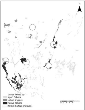
(2) 278. Here, we present an alternative approach, also based on the principles of rank modeling, that does not demand field measurements and uses only readily available geospatial data. Using these models, we were able to successfully rank the risk of finding elevated Hg concentrations in the flesh of two of the most praised fish species of the region, northern pike (Esox lucius) and walleye (Stizostedion vitreum), across a series of lakes located in the Abitibi-Témiscamingue region (ATr) (Province of Québec, Canada) that are subject to frequent fishing activities. The models were developed using Geographic Information System (GIS) and the model output was then used to produce Hg risk maps for local populations.. Material and methods Region under study The ATr covers an area of 64 878 km2, which represents about 5% of the territory of the Province of Québec (Canada). The region stretches over a 300 km along the N–S axis, and includes a variety of ecosystems. The widespread clay deposits found in the region were formed after the last ice age when Lake Ojibway-Barlow covered the region (Veillette et al. 1987). These lands constitute the largest proportion of agrarian soils found in the region. Due to its old volcanic origin, the region is also rich in mineral deposits, which sustain extensive mining activities for gold, copper and silver extraction. In addition to the mining and agriculture activities, the regional economy also depends on wood logging and processing. This study proposes a novel methodological approach to deal with the environmental issue of Hg in waterbodies at the regional scale using readily available geospatial data and appropriate statistical tools (Fig. 1). Fishing in the Abitibi-Témiscamingue region Fishing activities in the region can be divided into three types (FAPAQ 2002, Beaulne 2008).. Beaulne et al. • Boreal Env. Res. Vol. 17. The most important fish harvesting activity is sport fishing, with about 189 000 fishing days per year. The majority (55%) of fishers are nonlocal residents (FAPAQ 2002). Although sport fishers are not typically high-frequency fish consumers, they are still at risk of high Hg exposure through fish consumption, given that they usually prefer to eat large specimens (fish trophies), such as walleye and northern pikes, that also have the highest Hg concentrations (Lucotte et al. 2005). The second type fish harvesting activity is urban angling. Many of the 85 municipalities found in the ATr are located on the shores of lakes. Inhabitants of the small cities in these municipalities often take advantage of this favorable setting to regularly go fishing and thus acquire an important part of their dietary protein through fish consumption, making them at risk of high Hg intake (FAPAQ 2002, Lucotte et al. 2005). Finally, the third type of fishing activity is that of subsistence fishers from First Nations communities that settled long ago in the region. The ATr region is home to seven communities of the Algonquin Nation. The historic development and fate of the Algonquins are closely related to water plans and aquatic resources. These communities traditionally follow sustained fishing and hunting practices, making them by far the highest fish consumers in the province of Québec (Grenier et al. 1994, Lucotte et al. 2005). Contrarily to the other groups of fishers, the Algonquins usually diversify the type of fish consumed, including in their diet species with lower Hg concentrations such as whitefish and longnose suckers. Furthermore, the Algonquins are not subjected to the fishing regulation implemented in the region that forces fishers to release all walleye catches of less than 30 cm — corresponding to those usually bearing less Hg. Selection of the lakes to be included in the study An important part of the 20 000 lakes or so located in the ATr do not sustain any significant fishing activity due to limited access or their small size. These lakes were, therefore, removed.
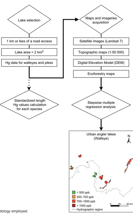
(3) Boreal Env. Res. Vol. 17 • Modeling mercury concentrations in fish: a GIS approach. 279. Lake selection. Maps and imageries acquisition. 1 km or less of a road access. Satellite images (Landsat 7). Lake area > 2 km2. Topographic maps (1:50 000). Hg data for walleyes and pikes. Digital Elevation Model (DEM) Ecoforestry maps. Standardized length Hg values calculation for each species. Stepwise multiple regression analysis. Urban angler lakes (Walleye). N. < 500 ppb. Fig. 1. Flow chart of the methodology employed.. from the dataset used in this study as they were considered irrelevant for establishing risk maps for local fishing populations. We limited our selection to lakes likely to be frequently used by either one of the three groups of fishers described above. The selection was performed as follows (Fig. 1): First, we analyzed the topographic and road and trail maps provided by the National Topographic Database (see http://geogratis.cgdi.. 500–700 ppb 700–1000 ppb > 1000 ppb Hydrographic region. 0. 25. 50 km. gc.ca/geogratis/en/index.html) to determine the extent of ground access to lakes. Lakes larger than 2 km2 located within 1 km from a road or trail were kept in our inventory. Then, lakes larger than 2 km2 located within a 5-km buffer zone of urbanized area (85 municipalities) were selected. Finally, lakes larger than 2 km2 located within a 10-km buffer zone of First Nation communities were also included in the analysis..
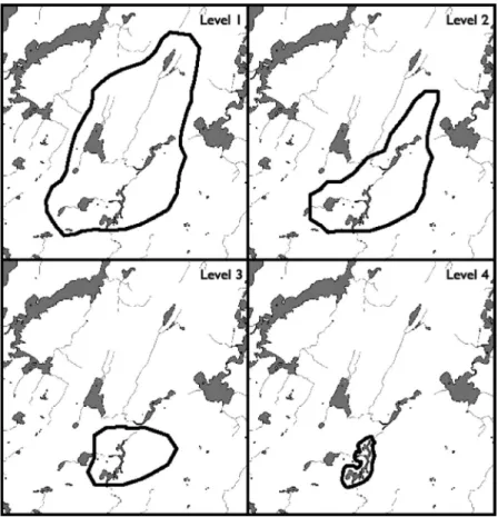
(4) 280. Beaulne et al. • Boreal Env. Res. Vol. 17. Fig. 2. Example of a lake watershed divided into four levels.. Choice of spatial range for the description of watersheds Biogeochemical processes at the watershed level are known to regulate Hg cycling. But it is likely that the impacts of such processes on Hg availability and loading will decrease with increasing distance from the lake shores. We thus divided lake watersheds into four levels in order to properly weight Hg-driving processes (Fig. 2). The 1st level watershed — an area up to 3000 km2 — is defined as the total land area draining either directly into a lake or into all higher rank lakes located upstream. The 2nd level watershed — an area up 1000 to km2 — represents the land area draining either directly into a lake, or into the first lake upstream. The 3rd level watershed — an area of tens to hundreds km2 — is limited to the land area draining directly into a lake, without transiting through another lake. Finally, the 4th level watershed comprises the land area within a 1-km buffer zone from the lakeshore.. These divisions were done using a total of 80 free-access topographic maps at a scale of 1:50 000 (http://geogratis.cgdi.gc.ca/geogratis/ en/index.html). The watershed limits for the 1st, 2nd and 3rd levels were hand drawn from topographic curves using the ArcMap software (©ESRI). The resulting watershed areas were validated, whenever possible, using Digital Elevation Models (DEM), analyzed using GRASS (Geographical Resources Analysis Support System), an open-source GIS software (Beaulne 2008). Selection of variables Based on the previous studies that describe Hg dynamics between watersheds and lakes (RouéLe Gall et al. 2005, Harris et al. 2007, Sacramento River Watershed Program 2002), we chose to include eleven variables and one composite variable (a ratio of two variables), seven.
(5) Boreal Env. Res. Vol. 17 • Modeling mercury concentrations in fish: a GIS approach. of which are applied to the four watershed levels used to model Hg concentrations found in fish tissue (Table 1). Geomorphological variables The ratio of watershed area (WA) to lake area (LA) and the drainage density (DD) were calculated using ArcMap. The WA/LA variable provides a good indication of the relative potential for Hg loading to lakes (Braga 2000, Roué-Le Gall et al. 2005). The DD indicates the efficiency with which Hg is transported from watersheds to lakes. This variable is calculated as the ratio of the total length of streams and rivers within a watershed to the total lake area. We used the approach proposed by Riera et al. (2000) to assign different lake orders within chosen drainage basins. The value of 0 is assigned to headwater lakes, and values from 1 to 4 correspond to the position of the lake in a chain of lakes, the value of 1 being assigned to the lake closest to the headwater lake. The lake assignment was performed with ArcMap, extracting the lake and river-stream layers from 1:50 000 maps (see http://geogratis.cgdi.gc.ca/ geogratis/en/index.html), and/or more detailed maps provided by the Bureau of Hydrological Resources of Quebec. There is little published information describing the impact that watershed slopes (WS) have on the efficiency of Hg transfer to lakes (Teisserenc et al. 2011). In this study, we analyzed the influence of different watershed slope intervals (0%–2%, 2%–6%, and > 6%) at the four, previously described, watershed levels. First, we analyzed a raster-based DEM with a resolution of 30 m pixel–1 (using ArcView Spatial Analysis) to estimate the WS variable. These data were then transformed into a vectorial representation in order to calculate the total watershed area corresponding to the WS values of 0%–2%, 2%–6%, and > 6%. The growth rate of fish appears to be a key variable in estimating Hg concentrations in fish flesh, especially for walleye (Lavigne et al. 2010). Since this information is not readily available for the lakes considered in this study, we instead used the presence/absence of clay. 281. substratum in the lakes as a proxy for slow/ fast growth rates for walleyes. We made this assumption based on the fact that clay lakes are more turbid, thus limiting the hunting capacity of a fish like walleye that rely on sight to catch their prey (Abrahams et al. 1997). This variable appears as “Clay” in Table 1. Mining activities are also quite frequent in the studied region. The variable “Mines” used in our models (Table 1) corresponds to the number of mining sites (including tailings) in the watersheds of the studied lakes. These were identified as such on the 1:50 000 maps (see http://geogratis.cgdi.gc.ca/geogratis/en/index.html). Land use and land cover variables Deforestation is known to enhance Hg transfer from the watershed to lakes (Garcia and Carignan 1999, Porvari et al. 2003, Garcia and Carignan 2005). It is for this reason that lakes a priori known to have watersheds affected by heavy logging activities in the few years prior to fish sampling were discarded from our analysis in order to establish fish Hg models for un-logged lakes only. Nevertheless, we later discovered that two lakes where recent logging activities had occurred were integrated into our dataset. Land cover classes were assigned using four matricial Landsat TM 7 satellite images Table 1. Variables considered in the establishment of the models. Geomorphological variables. Watershed area (WA, km2) Lake area (LA, km2). Drainage density (DD, km–1)* Lake order (Order, 1 to 5). Watershed slope (WS, 0%–2%, 2%–6%, > 6%)* Lake on the clay plain (Clay, yes/no) Land cover variables. Unforested vegetation area (UVA, %)*. Wetland (Wet, %)*. Bare soils (Bare, %)* Mature forested area (MFA, %)* Other Number of mine sites or mine tailings. in the watershed (Mine)* * Calculated for the four levels of watershed..
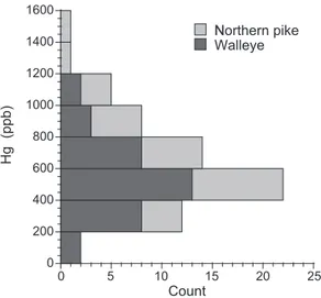
(6) 282. Fig. 3. Reference lakes with Hg concentrations readily available for pikes or/and walleyes.. with a 27-m resolution. The images were first mosaiced using GRASS software, and then land-cover classes were then determined with the unsupervised maximum likelihood analysis method using ArcGIS software. Four land cover classes were considered: (1) unforested vegetation areas (UVA) (regrouping cultivated land, low density shrubs and regenerating forest areas), (2) wetlands (Wet), (3) bare soils (Bare) (regrouping recently clear-cut areas, rock outcrops and human settlements), and (4) mature forested areas (MFA) (regrouping three of the ten classes yielded by the spectral analysis of the Landsat TM 7 images). The resulting regional land-cover classification was then transformed into a vectorial map (using ArcMap) and was analyzed with a layer of watersheds contours in order to calculate land cover areas corresponding to specific watersheds (Beaulne 2008). Fish data banks In order to build our northern pike and walleye Hg models, using information provided by the. Beaulne et al. • Boreal Env. Res. Vol. 17. Ministère du Développement Durable, de l’Environnement et des Parcs du Québec (www. mddep.gouv.qc.ca/Eau/guide), Hydro-Québec, and the Collaborative Mercury Research Network (COMERN) we gathered readily available fish Hg data for 27 lakes for pikes, and 33 lakes for walleyes (Fig. 3). These lakes cover the entire ATr region. Top predator northern pikes and walleyes are among the most valued catch (and fish meals) in the region, but they also usually bear the highest Hg concentrations. Hg concentrations at standardized fish length — 675 mm for northern pikes and 375 mm for walleyes — were calculated with polynomial regressions for each lake and each species using the approach presented by Lavigne et al. (2010) and Tremblay et al. (1998). However, the Québec Fish Consumption Guide (www.mddep.gouv.qc.ca/Eau/guide) only reports average fish Hg concentrations for small, average and large fish specimens i.e. 400 to 550 mm, 550 to 700 mm, and more than 700 mm for pikes, and 300 to 400 mm, 400 to 500 mm and more than 500 mm for walleyes. With this data, pike and walleye Hg concentrations at standardized length were calculated using second degree polynomial regressions. Pike Hg concentrations at 675mm standardized length ranged from 265 to 1409 ppb with an average value of 733 ppb whereas walleye Hg concentrations at 375 mm standardized length ranged from 170 to 1188 ppb with an average value of 585 ppb (Fig. 4). Model construction The first step in the design of models relating pike and walleye Hg concentrations and environmental variables was to run a stepwise multiple regression analysis using the JMPin software ver. 5.1 (SAS Institute 2003). The selected independent variables were LA and WA and the four land cover variables (MFA, UVA, Wet, Bare). A second set of independent variables included the lake order, WA/LA ratio, DD, the portion of the watershed area with a slope steepness of 0%–2%, 2%–6% and > 6% and the number of mines in the watershed. The data from all the lakes were used in the first stepwise regression analysis. Examination of the dispersion diagrams.
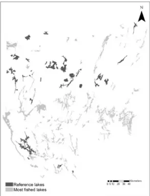
(7) Boreal Env. Res. Vol. 17 • Modeling mercury concentrations in fish: a GIS approach. Results Identification of the selected lakes A spatial analysis of the ATr identified 189 lakes in the region with a potential to sustain significant fishing activities, as they have a surface area larger than 2 km2 and are accessible via roads or trails. Only these lakes (Fig. 5) were selected for further analyses and modeling. Many of the 85 ATr municipalities are located on the shores of lakes and rivers. In fact,. 1600. Northern pike N Walleye. 1400 1200. Hg (ppb). between dependent and independent variables led us to segregate sub-groups of lakes and run a second series of multiple regression analyses for the walleye data only. These sub-groups include lakes with, or without, mining activities in their watershed, and lakes located on, or outside, the ancient Lake Ogibway-Barlow clay deposits. Underlying assumptions for regression analyses (linearity of relationships, normality of distributions, homoscedasticity of the residues) were verified (Scherrer 1984).. 283. 1000 800 600 400 200 0. 0. 5. 10. 15. Count. 20. 25. Fig. 4. Hg concentrations in 675 mm standardized length pikes and 375 mm standardized length walleyes.. there are 13 lakes with a surface area larger than 2 km2 that are located within a 5-km buffer zone around the towns and villages in the region, likely to be frequently visited by urban angers and sport fishers (Fig. 6). The ATr region is also home to seven First Nations communities, at. Fig. 5. All lakes (left-hand-side panel) and accessible lakes selected for the analysis (right-hand-side panel)..
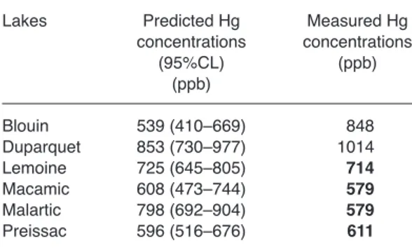
(8) Beaulne et al. • Boreal Env. Res. Vol. 17. 284. 1200 Hg = 341 + 98.5(Mines), r2 = 0.66. Hg (ppb). 1000. 800. 600. 400. 200. 3 4 5 6 7 Mines Fig. 7. Hg concentration in 675 mm standardized length pikes vs. number of mining sites and mine tailings located in the 4th level watershed.. Fig. 6. Lakes frequented by subsistance fishers, sport fishers and urban anglers.. higher risk of Hg exposure through frequent fish consumption: Pikogan, Kiticisakik, Lac Simon, Timiskaming, Winneway, Kebaowek and Hunter’s Point. Using spatial analysis we identified 19 lakes larger than 2 km2, located within 10 km of these settlements (Fig. 6). Northern pike Hg model The stepwise multiple regression analysis for the 27 lakes where northern pike Hg data were available indicates that only a few environmental variables correlate with Hg concentrations in pikes. The presence of wetlands in the watershed, for example is not related to Hg concentrations in pikes (r2 = 0.03, r2 = 0, r2 = 0.04 and r2 = 0 for the 1st to the 4th LW, respectively), even when atypical lakes with exceptionally low fish Hg concentrations, such as Lake Sabourin, are excluded from the analysis (r2 = 0.14, p = 0.0547). Similarly, no significant relationship between WA/LA — or DD — and northern pike Hg concentrations at standardized length was observed.. 0. 1. 2. However, the number of mining sites and mine tailings located in the 4th level watershed partly explains northern pike Hg concentrations, with 66% (p = 0.0074) of the variance being explained by this variable alone (Fig. 7). The portion of the watershed with gentle to moderate slope (steepness 2%–6%) also appears to be correlated with northern pike Hg concentrations, with the highest proportion (32%) of the variance being explained by the 3rd level watershed (p = 0.0016) (Fig. 8). The portion of mature forested area in the watershed also positively correlates with northern pike Hg concentrations, most notably for the 3rd level watershed where 28% of the variance is explained by this variable (p = 0.0044) (Fig. 9). Inversely, the proportion of bare soils, mostly corresponding to recently clear-cut areas, negatively correlates with northern pike Hg concentrations, although this correlation is weak (r2 = 0.13, p = 0.0798) (Fig. 10). Using the relationships presented above, we were able to build a predictive model explaining the Hg concentrations measured in northern pikes, according to the equation presented in Table 2. This simple model explains up to 74% (p < 0.0001) of the variance observed across northern pike Hg concentrations when data from two recently and extensively logged watersheds is removed — over a third of their total water-.
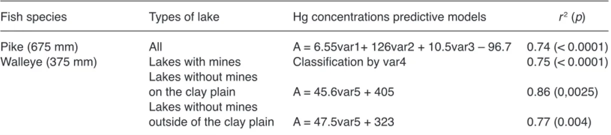
(9) Boreal Env. Res. Vol. 17 • Modeling mercury concentrations in fish: a GIS approach 1500. 285. 1600. 1200. Hg (ppb). Hg (ppb). 1000 800. 500 400 Hg = 341 + 6.48(Percentage of mature forest), r2 = 0.28. Hg = 510 + 8.5(Slope2%–6%), r2 = 0.32. 0. 30. 60 Slope2%–6%. 0. 90. Fig. 8. Hg concentration in 675 mm standardized length pikes vs. fraction of slopes between 2% and 6% in the 3rd level watershed.. shed area had been logged over the few years prior to the time the 2000 to 2003 satellite images were taken. We present in Table 3 an example of concordance between predicted and measured pike Hg concentrations in lakes where fish Hg data were available. Walleye Hg model The northern pike model fails to explain Hg concentrations measured in walleye tissue. In fact, when working with the walleye data we were not able to construct a single predictive model for the entire set of lakes used in this study and instead we had to separate lakes into three categories in order to obtain significant results. First, lakes having mining activities in the 4th. 0. 20 40 60 80 Percentage of mature forest. 100. Fig. 9. Hg concentration in 675 mm standardized length pikes vs. fraction of mature forest in the 3rd level watershed. 1500. 1000 Hg (ppb). 0. 500. 0. 0. 10. 20 30 40 50 Percentage of bare soil. 60. 70. Fig. 10. Hg concentration in 675 mm standardized length pikes vs. fraction of bare soils in the 3rd level watershed.. Table 2. Synthesis of the modeling results.Variables: var1 = fraction of mature forest in the 3rd level watershed, var2 = lake order, var3 = fraction of slopes between 2% and 6% in the 3rd level watershed, var4 = number of mining sites or mine tailings in the 4th level watershed, var5 = fraction of wetland in the 3rd level watershed. Fish species Types of lake Hg concentrations predictive models Pike (675 mm) All A = 6.55var1+ 126var2 + 10.5var3 – 96.7 Walleye (375 mm) Lakes with mines Classification by var4 Lakes without mines. on the clay plain A = 45.6var5 + 405 Lakes without mines. outside of the clay plain A = 47.5var5 + 323. r 2 (p) 0.74 (< 0.0001) 0.75 (< 0.0001) 0.86 (0,0025) 0.77 (0.004).
(10) Beaulne et al. • Boreal Env. Res. Vol. 17. 286. 1500. Hg = 96.4 + 233 (Mines), r2 = 0.75. Hg (ppb). 1200. 900. 600. 300. 0. 0. 1. 2. 3 Mines. 4. 5. 6. These lands are mainly used for agriculture or were used by settlers to establish towns and villages. In this group of lakes, the percentage of wetlands in the 3rd level watershed explains about 86% of the variability observed in the walleye Hg concentration dataset (p = 0.0025). The second group of lakes with no mining activity in their watershed includes lakes located outside the silt plain (surface deposits are till and drift) and mainly covered by forest. In this group of lakes, the percentage of wetlands on the 3rd level watershed similarly constitutes the strongest explanatory variable with 77% of the variance explained (p = 0.004) (Table 2).. Fig. 11. Hg concentrations for 375 mm standardized length walleyes vs. number of mines in the 4th level watershed.. Discussion. level watershed were identified. In this case, the number of lakeshore mines explains about 75% of the variability observed in the walleye Hg dataset (p < 0.0001) (Fig. 11 and Table 2). In lakes without any mining activity in the 4th level watershed, the fraction of wetland in the 3rd level watershed explains 73% of the variability of the Hg concentrations in walleyes. Better relationships are found when lakes without mines in their watersheds are split into two sub-groups. The first group comprises lakes located on the Ojibway-Barlow clay plain (more than 50% of the surface deposits is lacustrine silt), on the north-western part of the region.. This study presents for the first time a model to predict northern pike Hg concentrations using simple environmental variables easily derived from simple and available geographic data and satellite imagery. The advantage of the model is that it is readily usable on a wide regional scale and is functional even for large lake environments where in-situ environmental variables are difficult to evaluate properly. The first key variable in the northern pike model is the percentage of forested soils in the 3rd level watershed. This correlation is likely explained by the fact that the boreal landscapes have the ability to promptly capture important amounts of atmospheric Hg (Chen et al. 2005). The Hg burden then binds to organic material and can be lixiviated to lakes after episodes of rain or runoff (Driscoll et al. 2007, Chen et al. 2005). Indeed, recent studies have shown that new Hg inputs in boreal lakes are mostly linked to relatively fresh terrigenous organic matter, which originates from the surrounding watershed (Ouellet et al. 2009, Teisserenc et al. 2011). It is relevant to link the positive correlation of pike Hg concentrations with the percentage of forested soils in the 3rd level watershed to the weak negative correlation with the fraction of recently clear-cut areas in the lake watershed (Fig. 10). This observation is contrary to what previous studies reported for Hg levels found. Table 3. Comparison of predicted vs. measured Hg concentrations of 675 mm standardized length pikes for the lakes potentially fished by urban anglers. Numbers in boldface are measured values that fall within the calculated 95% confidence limits (95%CL). Lakes. Predicted Hg Measured Hg concentrations concentrations (95%CL) (ppb) (ppb). Blouin Duparquet Lemoine Macamic Malartic Preissac. 539 (410–669) 853 (730–977) 725 (645–805) 608 (473–744) 798 (692–904) 596 (516–676). 848 1014 714 579 579 611. Northern pike Hg model.
(11) Boreal Env. Res. Vol. 17 • Modeling mercury concentrations in fish: a GIS approach. in pikes caught in recently logged lakes (Garcia and Carignan 1999, 2005). One may explain this discrepancy by that fact that these authors sampled very small lakes (areas comprised between 0.1 and 2.3 km2) of the Boreal forest thus highly influenced by proportionally high percentage of clear-cut areas in their watersheds. Lake order, the second key variable, indicates the importance of Hg transfers from one lake to another in a chain of lakes. In fact, while most of the correlations presented here closely fit with variables scaled at the 3rd level watershed, the lake order takes into account Hg loading both from the primary watershed (3rd level watershed) and loading from upstream (2nd and 1st level watersheds). Finally, the importance of the third key variable, the percent of gentle to moderate slope steepness (2%–6%) in the watershed, may be explained by the fact that this range of steepness favors the transport of Hg bound to organic material from the surface soil horizons. Steeper slopes are usually more poorly vegetated while slopes with less than 2% steepness probably slow down lixiviation and Hg transport (Ouellet et al. 2009, Teisserenc et al. 2011). Contrary to previous findings reported in the literature (St. Louis et al. 1994, Roué-Le Gall et al. 2005, Harris et al 2007), variables such as DD, LA/WA or the fraction of wetlands were not significant in our statistical Hg models. This may be attributed to the fact that most of the previous models relied on data for perch, a fish species with a very different habit when compared with northern pike. Walleye Hg models Contrary to the northern pike dataset, it was impossible to elaborate a single predictive model for walleye Hg concentrations using the complete set of data. This is probably due to the ichthyologic differences between the two fish species. Walleyes prefer to feed in the pelagic zones of lakes, while northern pikes usually stay in shallow waters near the lakeshore. Lakes located on the clay plain have a higher turbidity than lakes located on the Canadian Shield. A predatory fish like walleye uses its sight to find. 287. preys and therefore has a slower growth rate in turbid lakes (Abrahams et al. 1997). As shown by Lavigne et al. (2010), growth rate is a key variable for explaining the Hg concentrations in walleye flesh. As fish age was not available in our fish data banks, we were not able to include this key variable in our model. To reduce the noise caused by this missing variable, we separated the lakes into two different groups, those on the clay plain and those outside of the clay plain. Three sub-models, supported by three key variables, were built to describe the observed variability of walleye Hg concentrations. The first key variable, the presence of mines in the 1st level watershed likely indicates anthropogenic point source Hg loadings that override other environmental processes controlling Hg concentrations. The second key variable, the surface deposits, segregates two other groups of lakes. In addition to differences possibly related to fish growth rates as mentioned above, it may be possible that the atmospheric Hg entering lake ecosystems located on the clay plain of ancient Lake Ogybway-Barlow loses part of its mobility and reactivity when binding with clay material, thus becoming less available for methylation (Jackson 1989, Dmytriw et al. 1995). The third key variable, the percent of wetland area in the 3rd level watershed, explains an important part of the variability in walleye Hg concentrations for lakes without mining activities, for lakes located both on and off the clay deposits (St. Louis et al. 1994). However the slope of the correlation between the two variables is significantly smaller for lakes located inside the clay deposits, supporting the hypothesis that Hg is partially immobilized through binding with clay particles. Regional mapping of the lakes potentially at risk of high Hg concentrations in fish Out of the 20 000 lakes located in the ATr, we identified 189 lakes in which significant fishing activities are likely to be undertaken by local inhabitants. For these lakes, we used the models generated in this study to draw regional maps showing predicted Hg concentrations in either.
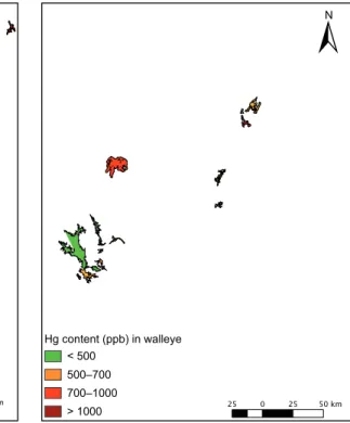
(12) Beaulne et al. • Boreal Env. Res. Vol. 17. 288 N. Hg content (ppb) in pike < 500. N. Hg content (ppb) in walleye < 500. 500–700. 500–700. 700–1000. 700–1000. > 1000. > 1000. Fig. 12. Regional predictive map of Hg concentrations for 675 mm standardized length pikes in lakes potentially frequented by sport fishers.. walleye or northern pike (Fig. 12). Such maps — which could be easily used by fishers — represent a powerful decision aid tool for community representatives and environmental stakeholders pointing out situations of potentially high exposure to Hg through fish consumption for the three groups of fishers identified in this study. The complete cartographic and GIS analysis allowed us to run the generated models on lakes where actual fish Hg data are not available. Another subset of 15 lakes used by subsistence fishers was also analyzed in order to predict fish Hg concentrations (Fig. 13). Considering the strategic importance of these lakes for the First Nation communities that extensively harvest fish resources from them, we were surprised to find Hg data for walleye available only for two of these lakes and only three lakes for northern pikes. Furthermore, the model output suggests that the highest northern pikes Hg concentrations found in the region are probably located in the lakes that are the closest to Algonquins settlements. Such a situation highlights the usefulness of our models for the identification of. Fig. 13. Regional predictive map of Hg concentrations in 375 mm standard length walleyes for lakes located nearby a native community.. Hg hot spots and sites where field data should be urgently collected.. Conclusions We were able to draw a regional portrait of the northern pike and walleye Hg concentrations in the ATr — a region that is representative of typical boreal forest environments — using easily derived geospatial data such as the fraction of mature forest area and wetlands in the watersheds, the lake order, the watershed slope steepness, and the presence of mining activities near lakeshores. Our results suggest that the Hg situation in the ATr is preoccupying. In only a few of the lakes considered in this study, Hg concentrations for the two highly valued fish species are predicted to be lower than the Canadian regulation on maximum Hg concentrations in retail fish (0.5 ppm). This conclusion also stresses the usefulness of visual decision aid tools, such as the one.
(13) Boreal Env. Res. Vol. 17 • Modeling mercury concentrations in fish: a GIS approach. developed in this study, that can help identify Hg hot spots and publicize this crucial information to community representatives and environmental stakeholders that frequently use fish resources. Finally, this study provides a good example of a successfully using GIS to elaborate a largescale ecosystem study based on previous findings issuing from more narrow and focused disciplinary research programs. It is likely that such a broader approach can be applied elsewhere to deal with environmental issues.. References Abrahams V.M. & Kattenfeld G.K. 1997. The role of turbidity as a constraint on predator–prey interactions in aquatic environments. Behavioral Ecology and Sociobiology 40: 169–174. Beaulne J.-S. 2008. Modélisation de la présence de Hg dans la chair des brochets et des dorés des lacs les plus pêchés de l’Abitibi-Témiscamingue: une approche par les systèmes d’information géographique. M.Sc. thesis, University of Québec at Montréal. Braga M.C., Shaw G. & Lester J.N. 2000. Mercury modeling to predict contamination and bioaccumulation in aquatic ecosystems. Rev. Environ. Contam. Toxicol. 164: 69–92. Chen C.Y., Stemberger R.S., Kamman N., Mayes B. & Folt C. 2004. Patterns of Hg bioaccumulation and transfer in aquatic food webs across. Multi-lake studies in the northeast US. Ecotoxicology 14: 135–147. Dmytriw R., Mucci A., Lucotte M. & Pichet P. 1995. The partitioning of mercury in the solid components of dry and flooded forest soils and sediments from a hydroelectric reservoir, Québec (Canada). Water Air Soil Pollut. 80: 1099–1103. Driscoll C., Han Y.-I., Chen C. & Evers D. 2007. Mercury contamination in forest and freshwater ecosystems in the northeastern United States. Bioscience 57: 17–28. Grenier A.-M., Dewailly É. & Gingras S. 1994. Étude pilote sur l’évaluation de l’exposition des pêcheurs sportifs au méthylmercure. Centre de santé publique de Québec. FAPAQ 2002. Plan de développement régional associé aux ressources fauniques de l’Abitibi-Témiscamingue. Société de la Faune et des Parcs du Québec, Direction de l’aménagement de la faune de l’Abitibi-Témiscamingue, Rouyn-Noranda, Quebec, Canada. [also available at http://www.mrnf.gouv.qc.ca/publications/faune/ PDRRF_08_211p.pdf]. Garcia E. & Carignan R. 1999. Impact of wildfire and clearcutting in the boreal forest on methyl mercury in zooplankton. Can. J. Fish. Aquat. Sci. 56: 339–345. Garcia E. & Carignan R. 2005. Mercury concentrations in fish from forest harvesting and fire-impacted Canadian boreal lakes compared using stable isotopes of nitrogen. Env. Toxicol. Chem. 24: 685–693. Harris R.C., Krabbenhoft D., Mason R., Murray M., Reash R.. 289. & Saltman R. 2007. Whole-ecosystem study shows rapid fish-mercury response to changes in mercury deposition. Proc. Natl. Acad. Sci. USA 104: 16586–16591. Jackson T.A. 1989. The influence of clay minerals, oxides and humic matter on the methylation and demethylation of mercury by micro-organisms in freshwater sediments. Applied Organometallic Chemistry 3: 1–30. Lavigne M., Lucotte M. & Paquet S. 2010. Fish growth rates as a mean for integrating environmental and biological factors controlling mercury concentration in predatory fish species. North American Journal of Fisheries Management 30: 1221–1237. Lucotte M., Canuel R., Boucher de Grosbois S., Amyot M., Anderson R., Arp P., Atikasse L., Carreau J., Chan H.M., Garceau S., Mergler D., Ritchie C., Robertson M.J. & Vanier C. 2005. An ecosystem approach to describe the mercury issue in Canada. In: Pirrone N. & Mahaffey K. (eds.), Dynamics of mercury pollution on regional and global scales: atmospheric processes, human exposure around the world, Springer Publisher, Norwell, MA, pp. 451–466. Ouellet J.-F., Lucotte M., Teisserenc R., Paquet S. & Canuel R. 2009. Lignin biomarkers as tracers of mercury sources in lakes water column. Biogeochemistry 94: 123–140. Petit S., Lucotte M. & Teisserenc R. 2011. Mercury sources and bioavailability in lakes located in the mining district of Chibougamau, Eastern Canada. Applied Geochemistry 26: 230–241. Porvari P., Verta M., Munthe J. & Haapanen M. 2003. Forestry practices increase mercury and methyl mercury output from boreal forest catchments. Environ. Sci. Technol. 37: 2389–2393. Riera J.L., Magnuson J., Kratz T. & Webster K.E. 2000. A geomorphic template for the analysis of lake districts applied to the Northern Highland Lake District, Wisconsin, USA. Freshwater Biol. 43: 301–318. Roué-Le Gall A., Lucotte M., Carreau J., Canuel R. & Garcia E. 2005. Development of an ecosystem sensitivity model regarding mercury levels in fish using a preference modeling methodology: application to the Canadian boreal system. Environ. Sci. Technol. 39: 9412–9423. Sacramento River Watershed Program 2002. Strategic plan for the reduction of mercury-related risk in the Sacramento River watershed. Available at http://www.srwp. org/documents/dtmc/documents/DTMCMercuryStrategyPlan.pdf. Scherrer B. 1984. Biostatistique. Gaétan Morin éditeur, Qc, Canada. St. Louis V., Rudd J.W.M., Kelly C.A., Beaty K.G., Bloom N.S. & Flett R.J. 1994. Importance of wetlands as sources of methyl mercury to boreal forest ecosystems. Can. J. Fish. Aquat. Sci. 51: 1065–1076. Teisserenc R., Lucotte M. & Houel S. 2011. TOM biomarkers as tracers of Hg sources in recent lake sediments of the Boreal forest. Biogeochemistry 103: 235–244. Tremblay G., Legendre P., Doyon J.F., Verdon R. & Schetagne R. 1998. The use of polynomial regression analysis with indicator variables for interpretation of mercury in fish data. Biogeochemistry 40: 189–201..
(14) 290 Veillette J.J. 1987. Former southwesterly ice flows in the Abitibi-Timiskaming region: implications for the con-. Beaulne et al. • Boreal Env. Res. Vol. 17 figuration of the Late Wisconsinan ice sheet. Earth Sci. Geol. Survey Can. 111–132..
(15)
Figure
+5
Documents relatifs