O
pen
A
rchive
T
OULOUSE
A
rchive
O
uverte (
OATAO
)
OATAO is an open access repository that collects the work of Toulouse researchers and
makes it freely available over the web where possible.
This is an author-deposited version published in :
http://oatao.univ-toulouse.fr/
Eprints ID : 10220
To cite this version : Bonometti, Thomas and Izard, Edouard and Lacaze,
Laurent Resolved simulations of submarine avalanches with a simple soft-sphere /
immersed boundary method. (2013) In: 8th International Conference on Multiphase
Flow - ICMF 2013, 26 May 2013 - 31 May 2013 (Jeju, Korea, Republic Of).
Any correspondance concerning this service should be sent to the repository
administrator: [email protected]
81h International Conference on Multiphase Flow ICMF 2013, Jeju, Korea, May 26-31, 2013
Resolved simulations of submarine avalanches
with a simple soft-sphere 1
immersed boundary method
Thomas Bonometti, Edouard Izard, Laurent Lacaze
IMFT, Université de Toulouse, INPT, UPS, CNRS, Institut de Mécanique des Fluides de Toulouse, Allée Camille Soula, F-31400 Toulouse, France
Keywords: immersed boundary, discrete element method, submarine avalanches, resolved simulations
Abstract
Physical mechanisms at the origin of the transport of solid particles in a fluid are still a matter of debate in the physics community. Y et, it is weil known that these processes play a fundarnental role in many natural configurations, such submarines landslides and avalanches, which may have a significant environmental and economie impact. The goal here is to reproduce the local dynamics of such systems from the grain scale to that of thousands of grains approxirnately. To this end a simple soft-sphere collision 1 immersed-boundary method has been developed in order to accurately reproduce the dynarnics of a
dense granular media collapsing in a viscous fluid. The fluid solver is a finite-volume method solving the three-dimensional, time-dependent Navier-Stokes equations for a incompressible flow on a staggered. Here we use a simple immersed-boundary method consisting of a direct forcing without using any Lagrangian marking of the boundary, the immersed boundary being defmed by the variation of a solid volume fraction from zero to one. The granular media is modeled with a discrete element method (DEM) based on a multi-contact soft-sphere approach. In this method, an overlap is allowed between spheres which mimics the elasto-plastic deformation of real grain, and is used to calculate the contact forces based on a linear spring model and a Coulomb criterion. Binary wall-particle collisions in a fluid are simulated for a wide range of Stokes number ranging from 10·1 to 104• lt is shown that good agreement is observed with available experimental results for the whole range of investigated parameters, provided that a local lubrication model is used when the distance of the gap between the particles is below a fraction of the particle radius. A new model predicting the coefficient of restitution as a function of the Stokes number and the relative surface roughness of the particles is proposed. This model, which makes use of no adjustable constant, is shown to be in good agreement with available experimental data. Finally, simulations of dense granular flows in a viscous fluid are performed. The present results are encouraging and open the way for a parametric study in the parameter space initial aspect ratio - initial packing.
Introduction
Particle-laden flows are encountered in a large number of industrial and natural applications, including chemical engineering, aeronautics, transportations, biomecanics, geophysics and oceanography. Modeling solid-fluid interaction is often difficult because of the complexity of the solid shape and motion in the fluid flow.
Methods for modeling solid-fluid interaction may be divided within two main groups, depending on the way the solid-fluid interfaces are described. One group, usually referred to as "body-fitted grid methods" makes use of a structured curvilinear or unstructured grid to conform the grid to the boundary of the fluid domain (Moin and Mahesh 1998; Hu et al. 2001). In situations involving complex moving boundaries, one needs to establish a new body-conformai grid at each time-step which leads to a substantial computational cost and subsequent slowdown of the solution procedure. In addition, issues associated with regridding arise such as grid-quality and grid-interpolation errors.
The second group of methods is referred to as "fixed-grid methods". These techniques make use of a fixed grid, which eliminates the need of regridding, while the presence of the
solid objects is taken into account via adequately formulated source terms added to fluid flow equations. Fixed-grid methods have emerged in recent years as a viable alternative to body-conformai grid methods. In this group, one can mention immersed-boundary method (IBM) (Peskin 2000; Fadlun et al. 2000; Kim et al. 2001; Uhlmann 2005), among others.
In the present work, we attempt to simulate the local dynarnics of such systems from the grain scale to that of thousands of grains approximately. To this end a simple soft-sphere collision 1 immersed-boundary method is
presented. The immersed-boundary method consists in a direct forcing method, using a continuous solid volume fraction to defme the boundary. The granular media is modeled with a discrete element method (DEM) based on a multi-contact soft-sphere approach.
The paper is structured as follow. First we describe the numerical techniques used here, then preliminary test cases are presented to show the ability of both methods independently. In a third part, binary wall-particle collisions in a fluid are simulated for a wide range of Stokes number ranging from 10·1 to 104, and a discussion about the use of a local lubrication model is done. In addition, a new model predicting the coefficient of restitution as a function of the
Stokes number and the relative surface roughness of the particles is proposed. Finally, simulations of dense granular flows in a viscous fluid are presented.
Nomenclature
gravitational constant (ms.2 ) pressure (Nm.2)
mean particle radius (rn) mean particle diameter (rn) local velocity in the fluid (ms-1) particle velocity (ms-1
)
local velocity in the particle (ms-1) IBM volume force (ms-2)
particle volume (m3) particle mass (kg)
coefficient of normal restitution contact time (s) Greek letters a Jl
v
psolid volume fraction dynarnic viscosity (Pas) kinematic viscosity (m2s-1) density (kg m-3 ) Subsripts p particle f fluid Numerical Approaches Immersed-boundary method (IBM)
Assuming a Newtonian fluid, the evolution of the flow is described using the Navier-Stokes equations, namely
V·V =0 (1)
p av+ pV.VV = -Vp
+
p g+V·
(u(vv +'VV)]+
P.f~ ~
where V, p, p and Jl are the local velocity, pressure, density and dynamic viscosity in the flow, respectively, g denotes gravity and
f
is a volume force term used to take into account solid-fluid interaction. (1)-(2) are written in a Cartesian or polar system of coordinates. These equations are enforced throughout the entire domain, comprising the actual fluid domain and the space occupied by the particles. In the following, the termf will be formulated in such way as to represent the action of the immersed solid boundaries upon the fluid.Let us consider a non-deformable solid particle of density pP, volume t?P and mass mP, the centroid of which being located at xP, moving at linear and angular velocity up and tq,, respectively. The local velocity U in the object is then defmed by U = uP + rxtq,, r being the local position relative the solid centroid. The motion of the particle is described by Newton's equations for linear and angular momentum of a rigid body, viz (Uhlmann 2005),
81h International Conference on Multiphase Flow ICMF 2013, Jeju, Korea, May 26-31, 2013
(3) with Fh
=-
v)P:_ )
f
fdt? p p "· (4) (5)where F h (resp. Ii.) is the acceleration (resp. torque) due to hydrodynarnic forces.
The time integration of the momentum equations for the fluid (2) and the solid (3) is performed via a third-order Runge-Kutta method for ail terms except the viscous term for which a second-order semi-implicit Crank-Nicolson scheme is used. The incompressibility condition (1) is satisfied at the end of each time step through a projection method. Domain decomposition and Message Passing Interface (MPI) parallelization is performed to facilitate simulation of large number of computational cells.
In general, the location of the particle surface is unlikely to coïncide with the grid nodes, so that interpolation techniques are usually employed to enforce the boundary condition by imposing constraints on the neighboring grid nodes. Here we adopt another strategy, by introducing a function a denoted as "solid volume fraction", which is equal to one in cells filled with the solid phase, zero in cells filled with the fluid phase, and 0 < a < 1 in the region of the boundary. In practice, the transition region is set-up to be of one-to-three grid cells approxirnately (Yuki et al. 2007). The forcing term reads
U-V
f=a--11t
(6)Recall that U is the local velocity imposed to the immersed solid object while V is the local velocity in the fluid; !::.t is the time step used for the time-advancement. The present choice, which may be viewed as a smoothing of the immersed boundary, is an alternative way to using a regularized delta function in conjunction with a Lagrangian marking of the boundary. The latter technique is largely used in immersed-boundary methods in order to allow for a smooth transfer of momentum from the boundary to the fluid (see e.g. Fadlun et al. 2000; Uhlmann 2005). The advantage of the present choice is that (1) it is simple to implement, (2) there is no need to introduce any Lagrangian mesh for tracking the immersed boundary, (3) no interpolation is performed so that the computational coast is reduced.
In the following, spherical particles will be considered. The corresponding solid volume fraction a is defined by (Yuki et al. 2007),
a(x)
=_!_ _ _!_tanh(lx
-xPI-
RJ
2 2
Â.ozi(7)
Π=
0.065 (1- )}
)+
0.39
(9)where n = (nx, ny, n,) is a normal outward unit vector at a surface element, u is a parameter controlling the thickness of the transition region and L1 is a characteristic grid size (.<1
=2112 .!U when the grid is uniform). Iso-contours of a as defined in (7) are shown in figure 2. With the present choices, the transition region is of three grid cells approximately.
Soft-sphere approach (DEM)
In this section, we describe the method used for dealing with solid contacts in a system of nP particles. Here, the modeling of the solid-solid interaction is done via a soft-sphere approach. Briefly, we assume the particles to be non-deformable but being able to overlap each other. This overlap is then used to compute the normal and tangential contact forces, using a locallinear mass-spring system and a Coulomb type mode!, respectively. When coupling is performed, an extra force Fe and torque
r;
is added in (3), namelyre= Iri
-
j
+Fwallf::ti
(10) (11)
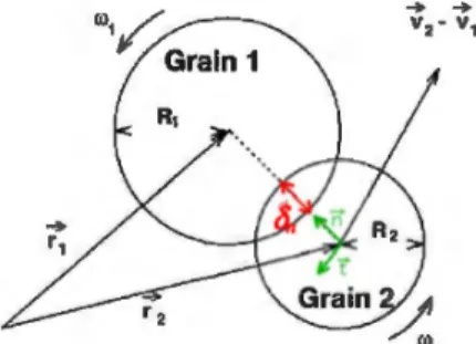
where F;1 is the contact force between particles i andj, F wau the wall-particle interaction force, F;1 and Fwau are the corresponding torques. F;.i and F;1 are computed using a local system of coordinates (n,t) depicted in figure 1 as follows Fi-i = F.n
+
FJri-j
= R;nx
Fl { 0 ifô.
>
0 F " = max ( 0,-k"ô" - Yn dt" dô ) otherwiseF,
=-min~k,ô,l,l,ucFn
l}sign(ôJ
(12) (13) (14) (15) where R; is the i-th particle radius,4. (
4) is the normal (tangential) distance of overlap, f1c is the friction coefficient,kn (k,) is the normal (tangential) stiffness and
rn
is the damping coefficient of the mass-spring mode!, respectively. Note that F wall and Fwa11 are treated in a similar manner by taking an infinite radius and mass for the wall. Theconstants of the mass-spring model y,, kn and k, are
calculated thanks to two additional parameters, namely the coefficient of normal restitution en and the contact time fe. These quantities are characteristic of the elastic properties of the particles.
81h International Conference on Multiphase Flow ICMF 2013, Jeju, Korea, May 26- 31, 2013
Figure 1: Notations used in the soft-sphere approach.
2m. ( )
Y,=--lne
n tc n (16) k = m.1!2+
T,
n 24
tc m. (17) where m.=m;mj(m;+mj) is the effective mass involved in the contact. Finall y, the tangential stiffness coefficient k, is assumed to be proportional to the normal stiffness coefficient kn (Foerster et al. 1994). In the present work, we set k,=0.2k.. To summarize, in the present soft-sphere approach, one needs to specify e., tc and Jlc in addition to the size and density of the particles for the mode! to be closed. Lubrication forceAs shown later, the coupled ffiM-DEM method may not be accurate in capturing the detailed flow structure in the liquid film which is drained when the particles approach each other because of the somewhat limited spatial resolution of the flow in the narrow gap. An extra lubrication force may thus be used in (3) to compensate for this (Kempe et al. 2012). Here we use the following mode! of lubrication force between two approaching particles i andj of velocity Up; and uPi and radius R; and Ri (Brenner 1961),
where 17 is an effective roughness length accounting for the surface roughness of real grains. This parameter was added in the model in order to mimic real particles and avoid the divergence of the force when contact occurs (4,=0). Depending on the type of material used for the particles, the relative surface roughness 1]/R is roughly in the range [10.6 ;
10"3] (Joseph et al. 2001). The present lubrication force is used when the distance between particles is in the range
0~4,~/2. We checked that the specifie value of the upper
bound of the force application (within the range [.!U; R]) did
not affect the results significantly. Results with the
Preliminary tests without coupling Falling sphere in a viscous liquid initially at rest
We set the physical properties of the particle and the fluid so the density ratio is P/P = 4 and the Archimedes number Ar= p(p -p)gD3
!,l
= 800. As shown later, this corresponds to a Re;uolds number, based on the terminal velocity of the sphere, of Re = pupl)lfl = 20 approximately. Here, we compare our results with those of a boundary-fitted approach which has been validated in previous papers (Mougin & Magnaudet 2001). This method fully resolves the flow around the falling sphere in the reference frame of the moving object, thanks to a spherical curvilinear grid which is refmed in the vicinity of the rigid boundary. The particle motion is solved via the Kirchhoff equations of motion. In this method a 88x34x66 spherical grid is used and the outer boundary are located at a distance of 20D from the sphere center.As for the present method, the simulation is performed in a cylindrical computational (r, z)-domain of 20D x 40D size with a 128 x 800 grid points. The spatial resolution is constant along the z-direction parallel to gravity as weil as in the region 0 $; r/D $; l.S (D/Ax = 20). For 1.S $; r/D $; 20, the grid size is varied following an arithmetic progression up to the outer wall. Free-slip boundary conditions are imposed at ali boundaries. The time-step used for the simulation is At( g/D /12 = 0.04. Figure 2 shows the grid used and iso-contours of the solid volume fraction a defmed in (7). The sphere is initially located at a distance SR from the upper wall and the fluid is initially at rest.
One can estimate the initial acceleration of the sphere at earl y times, assuming that only the buoyancy force and the added-mass force are at play. The initial vertical acceleration reads
dup = (Pp-P )g
dt Pp+CMP (19)
where CM is the added-mass coefficient equal to 112 for a sphere. When the sphere has reached a terminal velocity,_ the drag force is balanced by the buoyancy force so the tenmnal velocity can be computed as follows
lmp-mlg
u.p=
CvipnRz (20)where m p and m are the mass of the spherical particle and that of the fluid contained in an equivalent volume, respectively. Cv is the drag coefficient which can be classically estimated using Schiller and Naumann's correlation (Clift et al. 1978). Using this correlation together with the definition of the Reynolds number Re = pupl)lf1 and (20), one can compute the terminal velocity of the sphere. Figure 2 shows the temporal evolution of the sphere velocity with the boundary-fitted approach and the present immersed boundary method. For comparison, analytical solutions (19) and (20) are also plotted. Excellent agreement is observed with respect to both the numerical and analytical solutions. The present method is shown to satisfactorily reproduce the dynarnics of a free-moving object in a viscous fluid, from
ath International Conference on Multiphase Flow ICMF 2013, Jeju, Korea, May 26- 31, 2013 the acceleration phase up to the steady-state regime.
5 10 15
20
25t(g/D) 1/2
Figure 2: Time evolution of the particle velocity: - , present IBM method, - - -, boundary-fitted approach, ···, analytical solutions (19)-(20). Inset: close-up view of the grid used for the IBM simulation, with iso-contours of a= 0.01, 0.2S, O.S, 0.7S and 0.99.
Granular pressure in silo
In this section, only the soft-sphere approach is used, that is we solve (3) after having replaced Fh and
.n,
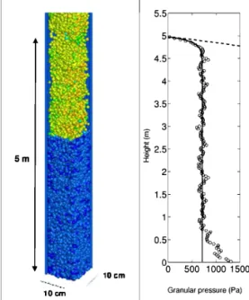
by F. and I;,, respective! y. This test case correspond to the filling of a silo of dimension 0.1x0.1xSm (figure 3) by S6000 particles of density p = 1317 kg.m·3 and mean radius R=Sxl0·3m under gravity !=9.81 m/s2• The radius is varied from one particle to another in a range of ±10% to avoid crystallization phenomena. Here we set the collision parameters to f1.=0.2S,en=0.3 and t.=104s. The walls of the silo were covered by fixed particles of equivalent size as those injected in the silo.
When the granular column is at rest, a coarse-graining technique is applied (see e.g. Goldhirsch & Goldenberg 2002) to measure the local granular stress tensor and the subsequent granular pressure (spherical part of the tensor). We plot on figure 3 the horizontally-averaged granular pressure in the silo. Going from the top of the column (z,.,Sm) down to the bottom (z=Om), the granular pressure fust follows a "hydrostatic" linear distribution on a depth corresponding to one silo diameter (4.9m $;
z
$; Sm), then the pressure quickly reaches a plateau and remains roughly constant on a distance of 4m down to z:=<0.7m. Below this height, the pressure monotonously increases as one gets to the bottom boundary. This behavior is attributed to the fact that in this region, particles have interacted with the bottom wall so the friction with the vertical wall was reduced and the pressure increased accordingly.The prediction of the granular pressure in the silo has been the subject of considerable work because of its obvious practical interest. One conventional model, namely the Janssen model, has proved to reproduce reasonably weil the pressure distribution in a silo. In this model one assumes that (i) the grain assembly is a continuous medium of equivalent density p8m=CpP, C being the global compactness
in the granular column, (ii) the vertical stresses are redistributed toward the horizontal directions by a factor K and (iii) the wall friction is at the threshold of motion. Under these assomption, the vertical distribution of the granular pressure reads,
5m ..._____ 10cm 5.5.---.---.---, 4.5 4 3.5 - 3
.s
~ 2.5 " I 2 1.5 0.5 500 1 000 1500Granular pressure (Pa)
Figure 3: Soft-sphere simulation. (Left) Silo filling with 56000 particles colorized by their velocity (blue: low velocity, red: high velocity). (Right) Horizontally-averaged granular pressure distribution in the silo (when the granular medium is at rest): 0, present DEM method, - , analytical solution (21), ---,equivalent hydrostatic distribution.
()
pgmgS[l
fw~(h-z))
p z = - - -
-e
fwKP
(21)where S (P) is the horizontal section (perimeter) of the silo,
fw is the wall friction coefficient, K is the coefficient of stress redirection and h is the height of the granular column. Note that the coarse-graining technique allows us to directly measure fw and K while these quantities are difficult to determine a priori or in a real experiment. Therefore, we plotted in figure 3 the analytical solution (21) by estimating the parameter fwK using a best fit of the numerical results.
This gives a value of fwK "" 0.30
±
0.06. The direct calculation of fwK from the numerical data gives, includingthe dispersion error,JwK "" 0.38 ± 0.11, a value which is in reasonable agreement with the best-fit estimate. This shows the capability of the present soft-sphere method to accurately reproduce the behavior of a dense granular media in motion and at rest.
Results and Discussion
Bouncing of a solid sphere on a wall in a viscous jluid
In this section, we present results of the simulation of one spherical particle bouncing on a wall in a viscous liquid initially at rest. To this end, the immersed boundary method (IBM) is coupled with the soft-sphere approach (DEM). The simulation is performed with the same grid as that used in figure 2. Here the resolution is D//'u = 20. Note that tests with D//'u = 10 and 40 have been done and showed that the
81
h International Conference on Multiphase Flow ICMF 2013, Jeju, Korea, May 26- 31, 2013 results were not affected by spatial resolution. Free-slip boundary conditions are imposed at ali boundaries except at the bottom wall where bouncing occurs. We set the physical properties of the particle and the fluid so that we cover a large range of density ratios 2~/p~102, Reynolds numbers
0.1~ Re=pupl)lp ~0(103) and Stokes numbers 1~t:;;104•
Here Stokes number is defined as,
(p
+CMp)VT DSt P (22)
9f.l
where CM=1/2 is the added-mass coefficient of the spherical particle.
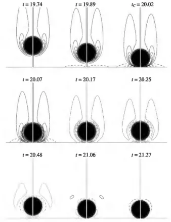
The evolution of the vorticity field around the particle during impact is presented in figure 4, for the case
P/P;=-8, St=53 and Re,.,60. Here the collision parameters
were set to en=0.97, tc=l0-4
s, f..Lr?0.25, and the relative surface roughness used in the lubrication model (18) was set to 1]IR=4xl04. At t=19.74, the flow field around the particle
is not influenced by the wall and vice versa. However, when the sphere gets doser to the wall, the fluid is pushed away from the centerline and vorticity is created at the wall. This is visible in figure 4 at time t=19.89 as the particle is at a distance from the wall of R approximately. Note that at this time instance, the grid resolution is of 4-5 grid cells in the liquid film. When collision occurs at t=20.02 ( 4,~0),
vorticity is maximum in the region close to the impact zone, indicating strong shear stress as fluid is pushed away parallel to the wall. Right after impact (20.07~t:;;20.25) a thin layer of vorticity of opposite sign develops at the particle surface and at the wall, while vorticity in the wake of the particle decreases, though still present. At t=20.48, the particle has reached its maximum height after the first bouncing and falls back again toward the wall. Afterwards
(t~21.06), the vorticity around the particle quickly disappear because of significant viscous dissipation.
The corresponding time evolution of the particle velocity is displayed in figure 5. Clearly, the particle reaches a steady-state velocity, denoted Vr, before bouncing on the wall. lt can be noticed that before the collision effectively occurs the particle velocity decreases from Vr to an impact velocity, denoted Vc, which is about 12% less than Vrin the present case. During the bouncing, the particle velocity changes sign but does not recover its initial velocity. This rebound velocity is denoted VR. Right after the impact, there is a strong decrease of the particle velocity followed by a milder trend. Finally, one can see on figure 5 a second rebound (1""21) which is hardly detectable from the flow visualization.
The simulation presented in figures 4 and 5 were first repeated for two specifie density ratios P/P;=-8 and 16
(Stand Re varying in the abovementioned range) and one
specifie Reynolds number Re=1, without any lubrication
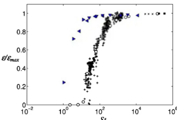
model (18). We plot in figure 6 the restitution coefficient
dG..ax=-VLIVr (see figure 5 for definitions) as a function of Stokes number (22). For comparison, we included available experiment data of the rebound of a spherical inclusion with a wall or another particle. While the numerical results are in good agreement with experimental data for St~200, the restitution coefficient is clearly overestimated at lower St. This can be attributed to the low resolution of the flow field when the gap between the particle and the wall is of the order of the grid size. As a consequence, the film pressure
stemming from the drainage of the liquid in the gap is underestimated so the particle rebound is artificially enhanced. This issue is overcome when one adds a lubrication force (18) in (3). Figure 7 shows the results obtained with the coupled IBM-DEM method with the lubrication mode! (18) for the case P/PF8. The numerical
results fall in the range of the experimental data.
t= 19.74 t = 19.89 tc= 20.02
t= 20.07 1=20.17 t = 20.25
t= 20.48 t = 21.06 t = 21.27
Figure 4: Vorticity field around a sphere impacting a wall
<PIPF8, St=53, Re,60, D/Liz=20.). Contours levels are set from -17.8 to 17.8 in increments of 3.9. Here, time and vorticity are scaled by (D!g/12 and (g!D/12 , respectively.
3,---~----~----~---~----, +-Vr
'
~ Vcô
9 ---a.0
0
:::l-1
-~9 20 21 +-VR-2
0
5
10
15
20
25
t(g/D) 1/2Figure 5: Temporal evolution of the particle vertical velocity (same case as figure 3). Inset: close-up view of the velocity during bouncing. Also defined are the particle terminal velocity Vr, the velocity at contact V c and the rebound velocity VR.
81h International Conference on Multiphase Flow ICMF 2013, Jeju, Korea, May 26- 31, 2013 Overall, one may conclude from figure 7 that the present IBM-DEM method is able to reproduce the rebound of a particle in a viscous fluid provided a suitable lubrication mode! is added to compensate the inability of the flow sol ver to capture the small scale flow field in the gap during the film drainage.
A new madel for the prediction of the effective coefficient of restitution
In this section, we propose a new mode! predicting the restitution coefficient E = -V
IIVr
observed in experiments without any adjustable constants. As shown later, this mode! only depends on two parameters, namely the Stokes number (22) and the relative surface roughness 1]/R. Sorne recent effort were done in attempting to predict the restitution coefficient thanks to models either based on lubrication theory (elasto-hydrodynamic madel, Davis et al. 1986, Barnocky & Davis 1988; mixed contact madel, Yang & Hunt 2008), or on a mass-spring analogy (Legendre et al. 2005, 2006). However, the first class of mode! fails to predict the restitution coefficient for the whole range of Stokes number, while the second class of model makes use of an adjusted constant.Here we revisit bath types of theory to derive a simple mode! which is able to capture reasonably well the observed restitution coefficients for the whole range of Stokes number (figure 7). The key idea is to decompose the sphere dynamics before and during impact into two stages. The first stage starts from a characteristic time at which the particle velocity begins to be influenced by the wall (i.e. for
§,.""R, approximately, see figures 4-5 and corresponding discussions) up to the time at which collision occurs (8,=0). During this stage, the particle is assumed (i) not to be deformed and (ii) to be slowed down by viscous forces generated by the displacement of fluid due to the presence of the wall. During the first stage, the particle velocity decreases from V1 to Vc, (see figure 5 for definition). In the
second stage, the particle get deformed and bounces. During this stage, we assume that the particle kinetic energy is converted into energy of deformation and is only partially restored into kinetic energy because sorne of the energy has been dissipated by bath inelastic deformation and viscous dissipation. During the second stage, the particle velocity goes from Veto VR.
In order to estimate the ratio V
dVr,
we consider that the particle, at location xP and of velocity uP, is moving toward a flat wall in a fluid at rest and we assume that the particle is subject to the steady drag force which is balanced by the buoyancy force, the added-mass force and the lubrication force F1ub defined in (18) which, in the present case, becomes F1ub=-61Cf.lU~/(8,.+1]). The kinematic equations then become,(23a,b)
where rn is the mass of the fluid contained in a sphere of radius R. Using the relation xP=R+§,., then dividing (23b) by (23a) in arder to eliminate time, and integrating between 4=0 (up=Vc) and 4=R (up=Vr), we find that
(24) where we assumed that R>>TJ. Regarding the second stage,
we follow Legendre et al. (2005)'s analysis and use a mass-spring model to describe the deformation
q
of the particle where we tak:e into account energy loss due inelastic deformation and viscous dissipation. The deformation of the particle is then govemed by,(25) with initial conditions §=0 and d!Jdt=Vc when the particle impacts the wall. Recall that
y,.
and kn are the damping andstiffness coefficient of the soft-sphere mass-spring model, respectively. C is a coefficient which we estimate to be inversely proportional to the relative surface roughness of the particle, i.e. C=RITJ. lntegrating (25) with the
corresponding initial conditions gives the classical solution
~t) of a damped harmonie oscillator (not shown), with a half-period of oscillation
(26)
(26) indicates that the larger the viscosity and/or
y,.,
the larger-r,
so that the contact time is larger accordingly, as expected. However, recent experiments of the impact of a solid sphere on a wall showed that the effective contact time remains finite and of the order of the contact time predicted by Hertz theory (considering no interaction with the surrounding fluid), in a large range of Stokes number 20:5:SK-103 (Legendre et al. 2006). Therefore, one can approximate (26) by ~((mp+CMm)lkn)112•Further assuming that the contribution of the lubrication force at impact 67!j.IR2V
dTJ
is of the same order as that of the elastic force knTJ in the dissipation of energy,one can estimate RITJ as a function of the fluid and particle
properties as RITJ=(k,/67!pVc)ll2. Using this together with
(26), the solution of (25) and the approximation
~((mp+CMm)lkn)112,
we can get an expression of the rebound velocity VR=d~ -r)ldt, as a function of the contact
velocity V c,
VR [ 1!/2 )
Vc = -e. exp
~Stx
fJ(St,TJI R) (27) fJ(St,q 1 R)= 1 + _!__1n(!l)
St R (28)
Combining (24), (27) and (28), we find a new model for the prediction of the coefficient of restitution êle,ax of a particle rebound in a fluid,
e
fJ(St,q!R)exp[ 1!/2 ) (29) ~ St x fJ(St,TJ 1 R)
emax
As mentioned above, this new model only depends on two parameters, namely Stand 1]/R. Note that here no adjustable
81h International Conference on Multiphase Flow ICMF 2013, Jeju, Korea, May 26 - 31, 2013 constant were needed. The model (29) is plotted in figure 7 for a wide range of relative surface roughness 10-6:5:1]/R:5:10-3. Good agreement is observed for both small and large values of the Stokes number. Note that the sensitivity of (29) with respect to 1]/R is larger at moderate-to-small Stokes numbers. This is line with the dispersion of experimental results which is observed to be larger at low St.
0.8 0.6 êlë,ax 0.4 0.2
..
o~---~~~oj+~~---~----~ 1~ 1~ 1~ 1~ 1~ StFigure 6: Restitution coefficient êlë,ax for spherical inclusions versus the Stokes number St. Present IBM-DEM simulations without lubrication force: T, p/p=16; <111111, p/p=8; ~. Rep"'l. Experiments with solid spheres: +, Joseph et al. 2001; 0, Gondret et al. 2002; x, Foerster et al. 1994. Experiments with drops: •, toluene drops in water (Legendre et al. 2005);
+,
liquid drop in air (Richard & Quéré 2000). Other experiments: •, spherical balloon filled with a mixture of water and glycerol (Richard & Quéré 2000). 0.8 0.6 êlë,ax0.4 0.2 o~----~~~j_~---~----~ 1~ 1~ 1~ 1~ 1~ StFigure 7: Same as figure 6:
+
,
present IBM-DEM simulations with lubrication force (18) for p/p=8. --, present model (29) with various relative surface roughnessw-
3:5:1JIR:5:10-6•
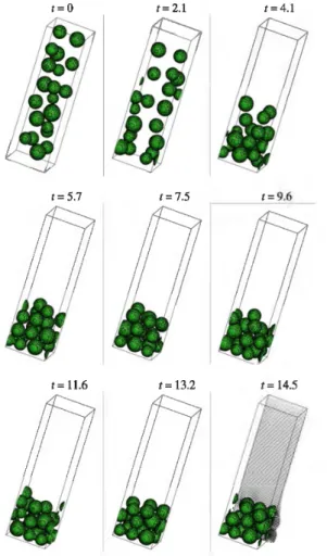
Immersed granular flow on an inclined plane
The last case corresponds to the simulation of an immersed granular flow on an inclined plane, as those encountered in submarine avalanches. The simulation is performed in a three-dimensional (x,y,z)-computational domain of size 3Dx3Dx10D in the streamwise, spanwise and vertical directions, respectively, discretized with 30X30x100 grid
points. We set the physical properties of the particle and the fluid so the density ratio is p/p = 85 and the Archimedes number Ar= p(pp-p)gD3!1i = 1200 (Re= puPD/p"' 10-100).
The collision parameters are the same as those used in figure 4. Periodic boundary conditions are imposed in the streamwise x-direction and no-slip boundary conditions are imposed elsewhere. The gravity vector makes an angle of 45° with the z-direction in the (x,z)-plane. Twenty quasi-monodispersed particles are initially randomly placed
in the computational domain within a fluid at rest.
Figure 8 shows the temporal evolution of the granular flow. The particles first collapse thanks to gravity (0 ::; t::; 5) to form a dense layer of particles which move as a sheet flow. The motion is sustained by the gravity since the angle of the inclined wall is weil above the angle of avalanche ("'30° for spherical particles). In that case, the fluid is put in motion by the displacement of the particle as observed in avalanches. The present results with a somewhat modest spatial resolution open the way for a parametric study in the parameter space initial aspect ratio - initial packing with a Iarger number of better-resolved particles.
Conclusions
We presented a simple soft-sphere immersed-bounday method capable of describing the flow of a dense granular media evolving in a viscous fluid. Simulations of wall-particle collisions in a fluid are shown to be in good agreement with available experimental results for the whole range of investigated parameters, provided that a local lubrication model is used. A new model predicting the coefficient of restitution as a function of the Stokes number and the relative surface roughness of the particles has been proposed and was shown to reproduce reasonably well experimental data. Finally, simulations of dense granular flows in a viscous fluid are presented. Current effort is made to perform a parametric study in the parameter space initial aspect ratio - initial packing, in order to investigate
immersed granular avalanches encountered in real
situations.
Acknowledgements
The authors thank Annaig Pedrono for her support in the development of the immersed-boundary version of the Navier-Stokes solver used in this research. Sorne of the computational time was provided by the Scientific
Groupment CALMIP (project P1027), the contributions of
which is greatly appreciated.
References
Barnocky, G. & Davis, R. H. 1988 Elastohydrodynamic collision and rebound of spheres: experimental verification. Phys. Fluids 31, 1324-1329.
Brenner, H. 1961 The slow motion of a sphere through a viscous fluid towards a plane surface. Chem. Eng Sei. 16, 242-251. Clift, R., Grace J. R. & Weber, M. E. 1978 . In Bubbles Drops and Panicules. Academie Press.
ath International Conference on Multiphase Flow ICMF 2013, Jeju, Korea, May 26- 31, 2013
1=0 1 = 2.1 1=4.1
1=11.6 t= 13.2 t= 14.5
Figure 8: Simulation of an immersed granular flow on a inclined plane in a viscous Iiquid. Time is scaled by (Dig)112• The grid resolution is made visible by lines plotted on the particles and the velocity field on a vertical plane at t=14.5.
Davis, R. H., Serayssol, J. M. & Hinch, E. J. 1986 The elastohydrodynamic collision of 2 spheres. J. Fluid Mech. 163, 479-497.
Fadlun, E. A., Verzicco R. Orlandi P. & Mohd-Yusof, J. 2000 Combined immersed boundary finite-difference methods for three-dimensional complex flow simulations. J. Comput. Phys.
161,35-60.
Foerster, S. F., Louge, M. Y., Chang, A. H. & Allia, K. 1994 Measurements of the collision properties of small spheres. Phys. Fluids 6, 1108-1115.
Goldhirsch, I. & C. Goldenberg, 2002 On the microscopie foundations of elasticity, Eur. Phys. J. E. 9, 245-251.
Gondret, P., M. Lance and L. Petit 2002 Bouncing motion of
spherical particles in fluid, Phys. Fluids 14, 643-652.
Hu, H., Patankar N. & Zhu, N. 2001 Direct numerical simulation of fluidsolid systems using the arbitrary lagrangian eulerian technique. J. Comput. Phys. 169, 427-462.
Joseph, G. , R. Zenit, L. Hunt and M. Rosenwinkel 2001 Particule-wall collisions in a viscous fluid, J. Fluid Mech. 433, 329-346.
Kempe, T. & J. Fohlich, 2012 Collision modelling for the interface-resolved simulation of spherical particules in viscous fluids, J. Fluid Mech, 709, 445 - 489.
Kim, J., Kim D. & Choi, H. 2001 An immersed-boundary finite-volume method for simulations of flow in complex geometries. J. Comput. Phys. 171, 132-150.
Legendre, D. C. Daniel and P. Guiraud 2005 Drop-wall bouncing in a liquid, Phys. ofFluids, 17,97-105.
Legendre, D., Zenit, R., C. Daniel and P. Guiraud 2006 A note on the modeling of the bouncing of spherical drops or solid spheres on a wall in viscous fluid, Chem. Eng. Sc. 61, 3543-3549.
Moin, P. & Mahesh, K. 1998 Direct numerical simulation: a tool in turbulence research. Ann. Rev. Fluid Mech. 30, 539--578.
Mougin, G. & Magnaudet, J. 2001 Path instability of a rising bubble. Phys. Rev. Lett. 88, 014502.
Peskin, C. 2000 The immersed boundary method. Acta Numerica
11, 479--517.
Richard, D. & Quéré D. 2000 Bouncing water drops. Eurphysics Letters 50, 769-775.
Uhlmann, M. 2005 An immersed boundary method with direct forcing for the simulation of particulate flows. J. Comput. Phys.
209, 448-476.
Yang, F.L. & M. L. Hunt, 2006 Dynaruics of a particule-particule collisions in a viscous liquid, Phys. Fluids 18, 121506.
Yuki, Y., Takeuchi S. & Kajishima, T. 2007 Efficient immersed boundary method for strong interaction problem of arbitrary shape object with self-induced flow. J. Fluid Sei. Tech. 2, 1-11.
81h International Conference on Multiphase Flow ICMF 2013, Jeju, Korea, May 26-31, 2013