Experiments on the Application of IOHMMs to Model Financial Returns Series

(1)

Montréal Mai 2002

Série Scientifique

Scientific Series

2002s-48

Experiments on the Application

of IOHMMs to Model Financial

Returns Series

Yoshua Bengio, Vincent-Philippe Lauzon,

Réjean Ducharme

(2)

CIRANO

Le CIRANO est un organisme sans but lucratif constitué en vertu de la Loi des compagnies du Québec. Le financement de son infrastructure et de ses activités de recherche provient des cotisations de ses organisations-membres, d’une subvention d’infrastructure du ministère de la Recherche, de la Science et de la Technologie, de même que des subventions et mandats obtenus par ses équipes de recherche.

CIRANO is a private non-profit organization incorporated under the Québec Companies Act. Its infrastructure and research activities are funded through fees paid by member organizations, an infrastructure grant from the Ministère de la Recherche, de la Science et de la Technologie, and grants and research mandates obtained by its research teams.

Les organisations-partenaires / The Partner Organizations

•École des Hautes Études Commerciales •École Polytechnique de Montréal •Université Concordia

•Université de Montréal

•Université du Québec à Montréal •Université Laval

•Université McGill

•Ministère des Finances du Québec •MRST

•Alcan inc. •AXA Canada •Banque du Canada

•Banque Laurentienne du Canada •Banque Nationale du Canada •Banque Royale du Canada •Bell Canada

•Bombardier •Bourse de Montréal

•Développement des ressources humaines Canada (DRHC) •Fédération des caisses Desjardins du Québec

•Hydro-Québec •Industrie Canada

•Pratt & Whitney Canada Inc. •Raymond Chabot Grant Thornton •Ville de Montréal

Short sections may be quoted without explicit permission, if full credit, including © notice, is given to the source.

ISSN 1198-8177

Les cahiers de la série scientifique (CS) visent à rendre accessibles des résultats de recherche effectuée au CIRANO afin de susciter échanges et commentaires. Ces cahiers sont écrits dans le style des publications scientifiques. Les idées et les opinions émises sont sous l’unique responsabilité des auteurs et ne représentent pas nécessairement les positions du CIRANO ou de ses partenaires.

This paper presents research carried out at CIRANO and aims at encouraging discussion and comment. The observations and viewpoints expressed are the sole responsibility of the authors. They do not necessarily represent positions of CIRANO or its partners.

(3)

Experiments on the Application of IOHMMs

to Model Financial Returns Series

*

Yoshua Bengio

†

, Vincent-Philippe Lauzon

‡

, and Réjean Ducharme

§

Résumé / Abstract:

"Input/Output Hidden Markov Models" (IOHMMs) sont des modèles de Markov cachés pour lesquels les probabilités d'émission (et possiblement de transition) peuvent dépendre d'une séquence d'entrée. Par exemple, ces distributions conditionnelles peuvent être linéaires, logistiques, ou non-linéaires (utilisant, par exemple, une réseau de neurones multi-couches). Nous comparons les performances de généralisation de plusieurs modèles qui sont des cas particuliers de IOHMMs pour des problèmes de prédiction de séries financières : une gaussienne inconditionnelle, une gaussienne linéaire conditionnelle, une mixture de gaussiennes, une mixture de gaussiennes linéaires conditionnelles, un modèle de Markov caché, et divers IOHMMs. Les expériences comparent ces modèles sur leurs prédictions de la densité conditionnelle des rendements des indices sectoriels et du marché. Notons qu'une gaussienne inconditionnelle estime le premier moment avec une moyenne historique. Les résultats montrent que, même si la moyenne historique donne les meilleurs résultats pour le premier moment, pour les moments d'ordres supérieurs les IOHMMs performent significativement mieux, comme estimé par la vraisemblance hors-échantillon.

Input/Output Hidden Markov Models (IOHMMs) are conditional hidden Markov models in which the emission (and possibly the transition) probabilities can be conditioned on an input sequence. For example, these conditional distributions can be linear, logistic, or non-linear (using for example multi-layer neural networks). We compare the generalization performance of several models which are special cases of Input/Output Hidden Markov Models on financial time-series prediction tasks: an unconditional Gaussian, a conditional linear Gaussian, a mixture of Gaussians, a mixture of conditional linear Gaussians, a hidden Markov model, and various IOHMMs. The experiments compare these models on predicting the conditional density of returns of market and sector indices. Note that the unconditional Gaussian estimates the first moment with the historical average. The results show that, although for the first moment the historical average gives the best results, for the higher moments, the IOHMMs yielded significantly better performance, as estimated by the out-of-sample likelihood.

Mots clés : Modèles de Markov cachés, IOHMM, séries financières, volatilité

Keywords: Input/Output Hidden Markov Model (IOHMM), financial series, volatility

*_{The authors would like to thank François Gingras, Éric Couture, as well as the NSERC Canadian funding agency.} †_{CIRANO et Département d'informatique et recherche opérationnelle, Université de Montréal, Montréal, Québec,} Canada, H3C 3J7. Tel: +1 (514) 343-6804, email: bengioy@iro.umontreal.ca

‡_{Département d'informatique et recherche opérationnelle, Université de Montréal, Montréal, Québec, Canada, H3C} 3J7. Email: lauzon@iro.umontreal.ca

§_{CIRANO et Département d'informatique et recherche opérationnelle, Université de Montréal, Montréal, Québec,} Canada, H3C 3J7. Tel: +1 (514) 343-6111 #1794, email: ducharme@iro.umontreal.ca

(4)

1 Introduction

Hidden Markov Models (HMMs) are statistical models of sequential data that have been used successfully in many machine learning applications, especially for speech recognition. In recent years, HMMs have been applied to a variety of applications outside of speech recognition, such as handwriting recognition (Nag, Wong and Fallside, 1986; Kundu and Bahl, 1988; Matan et al., 1992; Ha et al., 1993; Schenkel et al., 1993; Schenkel, Guyon and Henderson, 1995; Bengio et al., 1995), pattern recognition in molecular biology (Krogh et al., 1994; Baldi et al., 1995; Chauvin and Baldi, 1995; Karplus et al., 1997; Baldi and Brunak, 1998), and fault-detection (Smyth, 1994). Input-Output Hidden Markov Models (IOHMMs) (Bengio and Frasconi, 1995; Bengio and Frasconi, 1996) (or Conditional HMMs) are HMMs for which the emission and transition distributions are conditional on another sequence, called the input sequence. In that case, the observations modeled with the emission distributions are called outputs, and the model represents the conditional distribution of an output sequence given an input sequence. In this paper we will apply synchronous IOHMMs, for which input and output sequences have the same length. See (Bengio and Bengio, 1996) for a description of asynchronous IOHMMs, and see (Bengio, 1996) for a review of Markovian models in general (including HMMs and IOHMMs), and (Cacciatore and Nowlan, 1994) for a form of recurrent mixture of experts similar to IOHMMs.

An IOHMM is a probabilistic model with a chosen fixed number of states corresponding to different conditional distributions of the output variables given the input variables, and with transition probabilities between states that can also depend on the input variables. In the unconditional case, we obtain a Hidden Markov Model (HMM). An IOHMM can be used to predict the conditional density (which includes the expected values as well as higher moments) of the output variables given the current input variables and the past input/output pairs. The most likely state sequence corresponds to a segmentation of the past sequence into regimes (each one associated to one conditional distribution, i.e., to one state), which makes it attractive to model financial or economic data in which different regimes are believed to have existed.

Previous work on using Markov models to represent the non-stationarity in economic and financial time-series due to the business cycle are promising (Hamilton, 1989; Hamilton, 1988) and have generated a lot of interest and generalizations (Diebold, Lee and Weinbach, 1993; Garcia and Perron, 1995; Garcia and Schaller, 1995; Garcia, 1995; Sola and Driffill, 1994; Hamilton, 1996; Krolzig, 1997). In the experiments described here, the conditional dependency is not restricted to an affine form but includes non-linear models such as multi-layer artificial neural networks. Artificial neural networks have already been used in many financial and economic applications (see for example (Moody, 1998) for a survey), including to model some components of the business cycle (Bramson and Hoptroff, 1990; Moody, Levin and Rehfuss, 1993), but not using an IOHMM or conditional Markov-switching model. The main contribution of this paper is in showing a successful application of IOHMMs to a real-world financial data modeling problem, over different types of returns series, revealing some interesting properties of the underlying process by performing comparisons with alternative but related model structures. The IOHMMs and the other models are trained to predict the conditional density of the returns over the next one or more time steps (for daily, weekly,

(5)

and monthly data), not only their conditional mean. In this paper, we study and compare for different models the out-of-sample performance in terms of predicting the conditional density. Using the out-of-sample performance as a yardstick allows to compare models that have very different numbers of degrees of freedom, and that are not necessarily special cas-es of each other. The IOHMMs performed better in a statistically significant way in terms of out-of-sample log-likelihood in comparison to a Gaussian model, a HMM, a conditional linear Gaussian model, and a mixture of linear experts (mixture of conditionally linear Gaus-sian models). However, the GausGaus-sian model outperformed all the others for predicting the mean, and the IOHMMs performed better than models without a state variable, showing that the IOHMM captured non-linear dependencies in the higher moments involving a temporal structure, and that artificial neural networks were useful to capture these non-linearities.

2 Summary of the IOHMM Model and Learning

Algo-rithm

The model of the multivariate discrete time-series data is a mixture of several models, each associated to a sequence of states, or regimes. In each of these regimes, the relation between certain variables of interest may be different and is represented by a different conditional probability model. For each of these regime-specific models, we can use a multi-layer arti-ficial neural network or another conditional distribution model (depending on the nature of the variables). In this paper we experimented with conditionally Gaussian models for each regime, with the dependence being either linear or non-linear (with a neural network). The sequence of states (or regimes) is not observed, but it is assumed to be a Markov chain, with transition probabilities that may depend on the currently observed (or input) variables. In this paper we have only experimented with unconditional transition probabilities. An IOHMM is an extension of Hidden Markov Models (HMMs) to the case of modeling the conditional distribution of an output sequence given an input sequence. Whereas HMMs rep-resent a distribution P (yT

1) of sequences of (output) observed variables yT1 = y1, y2, . . . , yT,

IOHMMs represent a conditional distribution P (yT

1|xT1), given an observed input sequence

xT₁ = x1, x2, ..., xT. In the asynchronous case, the lengths of the input and output sequences

may be different. See (Bengio, 1996) for a more general discussion of Markovian models which include IOHMMs.

2.1 The Model and its Likelihood

As in HMMs, the representation of the distribution is very much simplified by introducing a discrete state variable qt (and its sequence q1T), and a joint model P (yT1, q1T|xT1), along with

two crucial conditional independence assumptions:

P (yt|qt1, y t−1 1 , x T 1) = P (yt|qt, xt) (1) P (qt+1|qt1, y1t, xT1) = P (qt+1|qt, xt) (2)

(6)

In simple terms, the state variable qt, jointly with the current input xt, summarize all

the relevant past values of the observed and hidden variables when one tries to predict the distribution of the observed variable yt, or of the next state qt+1.

Because of the above independence assumptions, the joint distribution of the hidden and observed variables can be much simplified, as follows:

P (yT₁, q₁T_|xT₁) = P (q1) T−1 Y t=1 P (qt+1|qt, xt) T Y t=1 P (yt|qt, xt) (3)

The joint distribution is therefore completely specified in terms of (1) the initial state prob-abilities P (q1), (2) the transition probabilities model P (qt|qt−1, xt) and, (3) the emission

probabilities model P (yt|qt, xt). In our experiments we have arbitrarily chosen one of the

states (state 0) to be the “initial state”, i.e., P (q1 = 0) = 1 and P (q1 > 0) = 0.

The conditional likelihood of a sequence, P (yT

1|xT1) can be computed recursively, by

computing the intermediate quantities P (yt₁, qt|xT1), for all values of t and qt, as follows:

P (yt₁, qt|xT1) = P (yt|qt, xt)

X

qt−1

P (qt|qt−1, xt)P (y1t−1, qt−1|xT1) (4)

The recursion is initialized with P (y1, q1|xT1) = P (y1|q1, x1)P (q1). This recursion is similar to

the one used for HMMs, and called the forward phase, but for the fact that the probabilities now change with time according to the input values. The computational cost of this recursion is O(T m) where T is the length of a sequence and m is the number of non-zero transition probabilities at each time step.

Let us note yTp

1 (p) for the p-th sequence of a training data set, of length Tp. The above

recursion allows to compute the log-likelihood function l(θ) =X p logP (yTp 1 (p)|x Tp 1 (p), θ) (5)

where θ are parameters of the model which can be tuned in order to maximize the likelihood over the training sequences _{xTp

1 (p), y Tp

1 (p)}. Note that we generally drop the conditioning of

probabilities on the parameters θ unless the context would make that notation ambiguous.

2.2 Training IOHMMs

For certain types of emission and transition distributions, it is possible to use the EM (Expectation-Maximization) algorithm (Dempster, Laird and Rubin, 1977) to train IOHMMs (see (Bengio and Frasconi, 1996) and (Lauzon, 1999)) to maximize l(θ) (eq. 5) iteratively. However, in the general case, one has to use a gradient-based numerical optimization algo-rithm to maximize l(θ). This is what we have done in the experiments described in this paper, using the conjugate gradient descent algorithm to minimize _{−l(θ). The gradient} ∂l(θ)_∂θ can be computed analytically by back-propagating through the forward pass computations (eq. 4) and then through the neural network or linear model. The equations for the gradients can be easily obtained, either by hand using the chain rule or using a symbolic computation program such as Mathematica.

(7)

2.3 Using a Trained Model

Once the model is trained, it can be used in several ways. If inputs and outputs up to time t (or just inputs up to time t) are given, one can compute the probability of being in each one of the states (i.e, regimes). Using these probabilities, one can make predictions on the output variables (e.g., decision, classification, or prediction) for the current time step, conditional on the current inputs and past inputs/outputs. This prediction is obtained by taking a linear combination of the predictions of the individual regime models,

P (yt|y1t−h, x t 1) = X i P (yt|qt= i, xt)P (qt= i, y1t−h|x t 1)

where h is called the horizon because it is the number of time steps from a prediction to the corresponding observation, i.e., we want to predict yt given yt−h (and the inputs). The

weights of this linear combination are simply the probabilities of being in each one of the states, given the past input/output sequence and the current input:

P (qt= i|xt1, y t−h 1 ) = P (qt= i, y1t−h|xt1) P iP (qt= i, y1t−h|xt1)

We can compute recursively

P (qt = i, yt−h1 |xt1) =

X

j

P (qt = i, qt−1 = j|xt)P (qt−1= j, yt−h1 |xt−11 )

starting from the P (q_t−h = i, yt₁−h_|xt₁−h) computed in the forward phase (equation 4).

We can also find the most likely sequence of regimes up to the current time step, using the Viterbi algorithm (Viterbi, 1967) (see (Lauzon, 1999) in the context of IOHMMs). The model can also be used as an explanatory tool: given both past and future values of the variables, we can compute the probability of being in each one of the regimes at any given time step t. If a model of the input variables is built, then we can also use the model to make predictions about the future expected state changes. What we will obtain is not just a prediction for the next expected state change, but a distribution over these changes, which also gives a measure of confidence in these predictions. Similarly for the output (prediction or decision) variables, we can train the model to compute the expected value of this variable (given the current state and input), but we can also train it to model the whole distribution (which contains information about the expected error in a particular prediction).

3 Experimental Setup

In this section, we describe the setup of the experiments performed on financial data, for modeling the future returns of Canadian stock market indices. The methodology for estimat-ing and comparestimat-ing performance is presented: it is based on the out-of-sample behavior of the models when trained sequentially. Using the out-of-sample performance allows to compare very different models, some of which may be much more parsimonious than others, and those

(8)

models do not need to be structurally special cases of each other. In subsection 3.1 we de-scribe the mathematical form of each of the compared models. In subsection 3.2, we explain how the out-of-sample measurements are analyzed in order to make a statistical comparison between a pair of models. The central question concerns the estimation of the variance of the difference between the average performance of two models.

Let us first introduce some notation. Let

rt= valuet/valuet−1− 1

be a discrete return series (the ratio of the value of an asset at time t over its value at time t_{− 1, which in the case of stocks includes dividends and capital gains). Let ¯r}h,t be a moving

average of h successive values of rt:

¯ rh,t = 1 h t X s=t−h+1 rs.

In the experiments, we will measure performance in two ways: looking at time t at how well the conditional expectation (first moment) of

yt= ¯rh,t+h

is modeled, and looking at how well the overall conditional density of yt is modeled. The

distribution is conditioned on the input series xt. The prediction horizons h in the various

experiments were 1, 5, and 12.

In the experiments, all the models ˆP are trained at each time step t to maximize the conditional likelihood of the training data, ˆP (y₁t−h_|xt₁−h, θ), yielding parameters θt. We then

use the trained model model to infer ˆP (yt|y1t−h, xt, θt), and we measure out-of-sample

• SE, the squared error: 1

2(yt− ˆE[yt|y t−h

1 , xt, θt])2, and

• NLL, the negative log-likelihood: − log ˆP (yt|y1t−h, xt, θt),

where ˆE[._{|θ] is the expectation under the model distribution ˆ}P (._{|θ). The above logarithm} is for making an additive quantity, and the minus is for getting a quantity that should be minimized, like the squared error.

In the experiments we have performed experiments on three types of return series: 1. Daily market index returns: we used daily returns data from the TSE300 stock

index, from January 1977 to April 1998, for a total of 4154 days. In some experiments daily returns are predicted while in others the daily data series are used to predict returns over 5 days (i.e. one week since there are no measurements for week-ends). 2. Monthly market index returns: we used 479 monthly returns from the TSE300 stock

index, from February 1956 to January 1996. We also used 24 economic and financial time-series as input variables in some of the models.

3. Sector returns: we used monthly returns data for the main 14 sectors of the TSE, from January 1956 to June 1997 inclusively, for a total of at most 497 months (some sectors started later).

(9)

3.1 Models Compared

In the experiments, we have compared the following models. All can be considered special cases of IOHMMs, although in some cases an analytic solution to the estimation exists, in other cases the EM algorithm can be applied, while in others only GEM or gradient-based optimization can be performed.

• Gaussian model: we have used a diagonal Gaussian model (i.e., not modeling the covariances among the assets). The number of free parameters is 2n for n assets. In the experiments n = 1 (TSE300) or n = 14 (sector indices). There is an analytical solution to the estimation problem. This model is the basic “reference” model to which the other models will be compared.

Pg(Y = y|x, θ) = n

Y

i=1

N (yi; µi, σi2)

where N (x; e, v) is the Normal probability of observation x with expectation e and variance v, θ = (µ, σ), and µ = (µ1, . . . , µn), σ = (σ1, . . . , σn). This is like an

“uncondi-tional” IOHMM with a single state.

• Mixture of Gaussians model: we have used a 2-component mixture in the experi-ments, whose emissions are diagonal Gaussians:

Pm(Y = y|x) = J

X

j=1

wjPg(Y = y|x, pj)

where θ = (w, p1, p2, ..., pJ), pj is the vector with the means and deviations for the j-th

component, and P

jwj = 1, wj ≥ 0. J = 2 in the experiments, to avoid overfitting.

The number of free parameters is J_{− 1 + 2nJ. This is like an “unconditional” IOHMM} with J states and shared transition probabilities (all the states share the same tran-sition probability distribution to the next states). This means that the model has no “dynamics”: the probability of being in a particular “state” does not depend on what the previous state was.

• Conditional Linear Gaussian model: this is basically an ordinary regression, i.e., a Gaussian whose variance is unconditional while its expectation is conditional:

Pl(Y = y|x, θ) = n Y i=1 N (yi; bi+ K X k=1 Ai,kxk, σi2)

where θ = (A, b, σ), xk denotes the k-th element of the input vector. The number of

free parameters is n(2 + K). In the experiments, K = 1, 2, 4, 6, 14, or 24 inputs have been tried for various input features. See more details below in section 4.

• Mixture of Conditional Linear Gaussians: this combines the ideas from the pre-vious two models, i.e., we have a mixture, but the expectations are linearly conditional

(10)

on the inputs. We have used separate inputs for each sector prediction: Plm(Y = y|x, θ) = J X j=1 wjPl(Y = y|x, pj)

where θ = (w, p1, p2, . . . , pJ), pj is the parameter vector for a conditional linear Gaussian

model, and as usual wj ≥ 0, Pjwj = 1. The number of free parameters is J times the

number of free parameters of the conditional linear Gaussian model, i.e., nJ (2 + K) in the experiments. J = 2 in the experiments, and K = 1, 2, 4, 6, 14, 24 have been tried. This is like an IOHMM whose transition probabilities are shared across all states. Like for the mixture of Gaussians, this means that the model has no “dynamics”: the probability of being in a particular “state” does not depend on what the previous state was. Note that this model is also called a mixture of experts (Jacobs et al., 1991). • HMM: this is like the Gaussian mixture except that the model has dynamics, modeled

by the transition probabilities. In the experiments, there are J = 2 states. The number of free parameters is 2nJ +J (J_{−1). This is like an “unconditional” IOHMM. Each} emis-sion distribution is an unconditional multinomial: P (qt = i|qt−1 = j, xt) = Ai,j. Each

emission distribution is a diagonal Gaussian: P (yt|qt= i, xt) =Qj=1n N (yt,i; µj,i, σ2j,i).

• Linear IOHMM: this is like the mixture of experts, but with dynamics (modeled by the transition probabilities), or this is like an HMM in which the Gaussian expectations are affine functions of the input vector. We have not used conditional transition probabilities in the experiments. Again we have used J = 2 states, and the number of inputs K varies. The number of free parameters is nJ (2 + K) + J (J _{− 1).}

• MLP IOHMM: this is like the linear IOHMM except that the expectations are non-linear functions of the inputs, using a Multi-Layer Perceptron with K inputs and a single hidden layer with H hidden units (H = 2, 3, ... depending on the experiment). In one set of experiments we have used the same MLP for all the n assets (i.e., a single network per state is used, with n outputs associated to the n assets). In the other experiments, a separate network (with 1 output and K inputs) is used for each asset, so there are n MLPs per state. In the first case the number of free parameters is J (J _{− 1) + J(2n +} (1 + H)n + H(n + 1)), and in the second case it is J (J _{− 1) + Jn(2 + H + H(K + 1)).}

3.2 Performance Measurements

When comparing the out-of-sample performance of two predictive models on the same data, it is not enough to measure their average performance: we also need to know if the performance difference is significant. In this section we explain how we have answered this question, using an estimator of the variance of the difference in average out-of-sample performance of time-series models.

In the experiments on sectors, there are several assets, with corresponding return series. Different models are trained separately on each of the assets, and the results reported below concern the average performance over all the assets. We have measured the average squared

(11)

error (MSE) and the average negative log-likelihood (NLL). We have also estimated the vari-ance of these averages, and the varivari-ance of the difference between the performvari-ance for one model and the performance for another model, as described below. Using the latter, we have tested the null hypothesis that two compared models have identical true generalization. For this purpose, we have used an estimate of variance that takes into account the dependencies among the errors at successive time steps. Let et be a series of errors (or error differences),

which are maybe not i.i.d. Their average is

¯ e = 1 n n X t=1 et,

assumed approximately Normal. We are interested in estimating the variance

V ar[¯e] = 1 n2 n X t=1 n X t0₌₁ Cov(et, et0).

Note that et’s form a series of out-of-sample performances, and unlike a series of in-sample

residues it may have autocorrelations, even if the model has been properly trained. A plot of the auto-correlation function of et (both for the NLL sequence and the difference in NLL

for two models) show the presence of significant auto-correlations. Since we are dealing with a time-series, and because we do not know how to estimate independently and reliably all the above covariances, we assumed that the error series is covariance-stationary and that the covariance dies out as _{|t − t}0_{| increases.}

Because there are generally strong dependencies between the errors of different mod-els, we have found that much better estimates of variance were obtained by analyzing the differences of squared errors, rather than computing a variance separately for each average:

V ar[¯eA_i _{− ¯e}B_i ] = V ar[¯eA_i ] + V ar[¯eB_i ]_{− 2Cov[¯e}A_i , ¯eB_i ] where ¯eA

i is the average error of model A on asset i, and similarly for B. Note that to take the

covariance into account, it is not sufficient to look at the average out-of-sample performance for each model.

The average over assets of the performance measure is simply the average of the average errors for each asset:

¯ eA = 1 n n X i=1 ¯ eA_i .

To combine the variances obtained as above for each of the assets, we decompose the variance of the average over assets as follows:

V ar[1 n n X i=1 (¯eA_i _{− ¯e}B_i )] = 1 n2 n X i=1 V ar[¯eA_i _{− ¯e}B_i ] + 2 n2 n X i=1 X j<i

Cov[¯eA_i _{− ¯e}B_i , ¯eA_j _{− ¯e}B_j ]

where the covariances are estimated by the sample covariances of the averages of the error differences:

Cov[¯eA_i _{− ¯e}B_i , ¯eA_j _{− ¯e}B_j ]_≈ 1 T (T _{− 1)}

T

X

t=1

(12)

In the tables below, we give the p-value of the null hypothesis that model A is not better than model B (where model A is a reference model, such as the best-performing model). In the case that ¯eA < ¯eB, the alternative hypothesis is that A is better than B (so we use a single-sided test, with p-value = P (E[eB_]_{− E[e}A_] _{≥ ¯e}B _{− ¯e}A_{)). In the opposite case, we}

consider the converse test (with the alternative hypothesis being that B is better than A).

4 Experimental Results

Each of the tables in this section gives the result of a series of experiments in which the output variable is the same, and we vary the choice of model and input variables (when the model is conditional).

To explain some of the details of the input variables used in the experiments, let us define the following measure of return variation:

vt =|rt− ¯rt,t|

where ¯rt,tis the historical average of the returns up to time t, and ¯vd,tis a d-time steps moving

average of vt available at time t.

The following target output variables have been considered:

• TSE300 5-day return: we want to predict the conditional density of the 5-day average future market index return yt= ¯r5,t+5 at time t (t on a daily scale); horizon h = 5.

• TSE300 12-month return: we want to predict the conditional density of the 1-year average future market index return yt= ¯r12,t+12at time t (t on a monthly scale); horizon

h = 12.

• TSE300 1-month return: we want to predict the conditional density of next month’s market index return yt = rt+1 at time t (t on a monthly scale); horizon h = 1.

• 14 sectors 1-month return: we want to predict the individual conditional density of next month’s return for each of the 14 sector indices of the Toronto Stock Exchange, yt= rt+1, at time t (t on a monthly scale); horizon h = 1.

The following input variables have been considered in the experiments (when the number of inputs used is n, it is shown in the tables with K = n besides the model structure):

• 1 input: the current return rt associated to the output series.

• 2 inputs: the current return rt and current variation vt.

• 4 inputs: the current return rt, current variation vt, and the average past 4 returns

and variations ¯r4,t and ¯v4,t.

• 12 inputs: the current return rt, current variation vt, the average past 4 returns and

(13)

• 14 inputs: the 14 current sector returns.

• 24 inputs: 24 economic and financial indicators of the Canadian financial markets: the first input is the historical average of the TSE300 market index, the next two variables are two Canadian interest rates, the next 6 variables are estimated risk premia for various assets, the next 2 variables are two measures of return-on-equity for the Canadian market, and the last 13 provide the shape of the interest rate curve.

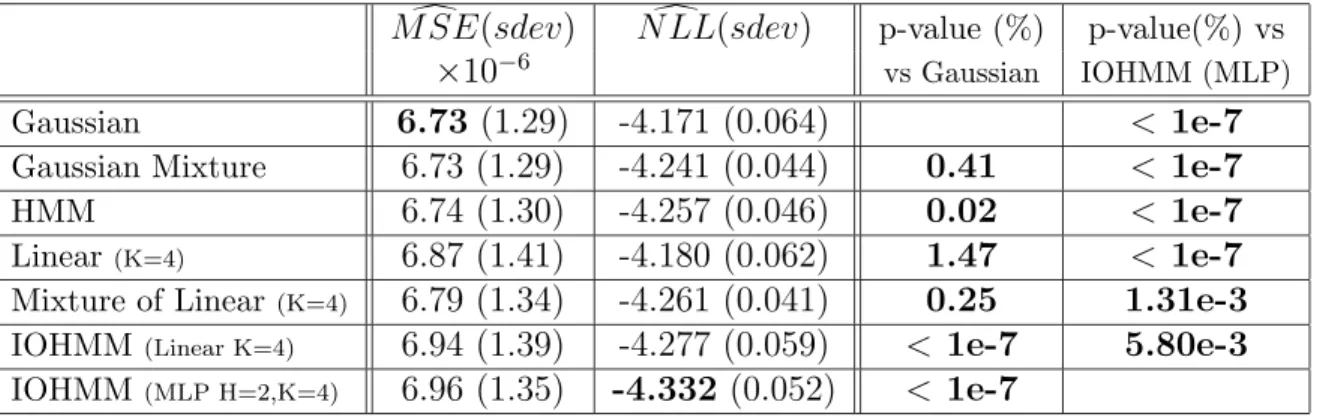
In the tables, the column entitled “M SE(sdev)” gives the average squared error and thed

estimated standard deviation of that average (in parenthesis). A similar column is provided for the negative log-likelihood (NLL). The performance figure in bold is the lowest (i.e. the best) in the column. The column entitled “p-value (%) vs Gaussian” gives the p-value (in percent) of a single-sided test for the null hypothesis that the model is not better in NLL than the Gaussian reference. If there is no “W” before the percentage, the alternative hypothesis is that the model is better than the reference; if there is a “W” then the test is with respect to the alternative hypothesis that the reference is better than the model. Similarly, the column entitled “p-value (%) vs M” compares each of the model with model M (which is the one with the lowest NLL). For this column there never is a “W” since the comparison is always against the “best” model, so we are testing with respect to the alternative hypothesis that the given model is worse than the “best” model. For both p-value columns, bold figures underline the fact that the p-value is less than 5%, i.e., that we consider that the null hypothesis of no difference should be rejected. Since in all comparisons no model significantly improved on the Gaussian for predicting the first moment (i.e., with respect to mean squared error), we have only given the p-values for comparing the negative log-likelihoods. Note that the p-values take into account not only the variances of each model’s performance but also their covariance, which is generally positive (hence the variance of their difference is much smaller than the sum of their variance).

d

M SE(sdev) N LL(sdev)d p-value (%) p-value(%) vs

×10−6 _{vs Gaussian} _{IOHMM (MLP)}

Gaussian 6.73 (1.29) -4.171 (0.064) < 1e-7

Gaussian Mixture 6.73 (1.29) -4.241 (0.044) 0.41 < 1e-7

HMM 6.74 (1.30) -4.257 (0.046) 0.02 < 1e-7

Linear(K=4) 6.87 (1.41) -4.180 (0.062) 1.47 < 1e-7

Mixture of Linear(K=4) 6.79 (1.34) -4.261 (0.041) 0.25 1.31e-3

IOHMM(Linear K=4) 6.94 (1.39) -4.277 (0.059) < 1e-7 5.80e-3

IOHMM(MLP H=2,K=4) 6.96 (1.35) -4.332 (0.052) < 1e-7

Table 1: Results on modeling the next TSE300 5-day returns every day. Bold MSE or NLL shows the best value obtained. Bold p-values are < 5%, suggesting that the difference with the reference is significant.

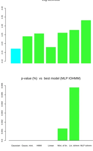
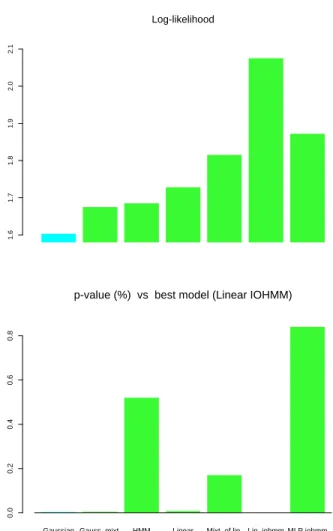
In table 1 and figure 1 the results on predicting the 5-day return of the TSE300 are presented. All the conditional models use the 4 inputs variables. No model outperforms

(14)

4.10 4.15 4.20 4.25 4.30 4.35 4.40 Log-likelihood

Gaussian Gauss. mixt. HMM Linear Mixt. of lin. Lin. iohmm MLP iohmm

0.0 0.001 0.002 0.003 0.004 0.005 0.006

p-value (%) vs best model (MLP IOHMM)

Figure 1: Comparative results on modeling the conditional density of the next TSE300 5-day returns every day. Top: out-of-sample log-likelihood. Bottom: p-value vs MLP IOHMM.

(15)

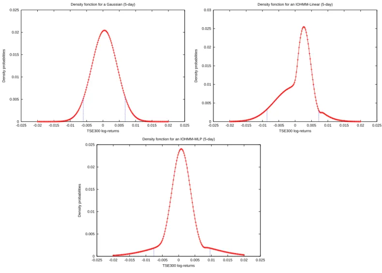
the Gaussian for predicting the first moment, but all of them outperform the Gaussian for predicting the conditional density. As in all of the other experiments, the Gaussian model gives the lowest MSE (error in prediction of the first moment), but the difference with the other models is not significant. For predicting the conditional density, the best model is the non-linear IOHMM (with a MLP), and the difference with each of the other models is significant. The following differences are also significant: the HMM is significantly better than the Gaussian mixture (p-value = 1.1%, showing that state information is important), the conditionally linear mixture is significantly better than the unconditional mixture (p-value = 0.16%, showing that the inputs are useful to predict the distribution of the future returns) and the linear IOHMM is significantly better than the mixture of conditionally linear mixture (p-value = 2.54%, showing that even with conditioning inputs, the hidden state variable remains useful). In addition, the table shows that the non-linearity in the IOHMM is important to get further improvement (it is not always the case with the other data sets). In figure 2 are shown examples of the shape of the predicted conditional densities for three of the models, out-of-sample, on this data series. Note the flatter shape of the density for the two IOHMMs (around 1 to 2% change in price).

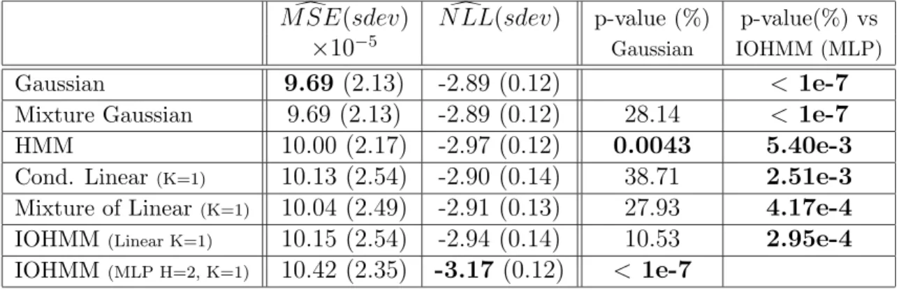
d

M SE(sdev) N LL(sdev)d p-value (%) p-value(%) vs

×10−5 _Gaussian _{IOHMM (MLP)}

Gaussian 9.69 (2.13) -2.89 (0.12) < 1e-7

Mixture Gaussian 9.69 (2.13) -2.89 (0.12) 28.14 < 1e-7

HMM 10.00 (2.17) -2.97 (0.12) 0.0043 5.40e-3

Cond. Linear(K=1) 10.13 (2.54) -2.90 (0.14) 38.71 2.51e-3

Mixture of Linear (K=1) 10.04 (2.49) -2.91 (0.13) 27.93 4.17e-4

IOHMM(Linear K=1) 10.15 (2.54) -2.94 (0.14) 10.53 2.95e-4

IOHMM(MLP H=2, K=1) 10.42 (2.35) -3.17 (0.12) < 1e-7

Table 2: Results on modeling the next TSE300 12-month returns every month. Bold MSE or NLL shows the best value obtained. Bold p-values are < 5%, suggesting that the difference with the reference is significant.

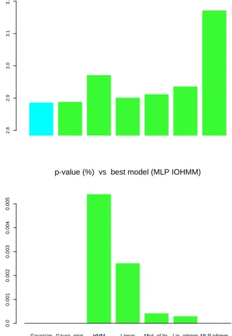
In table 2 and figure 3, the results of experiments on the monthly TSE300 data are pre-sented, with a horizon of h = 12 months, i.e., the models predict every month the conditional density of the next 12-month TSE300 market index return. Note that only the non-linear IOHMM and the HMM give a significantly better model than the Gaussian, and note that the non-linear IOHMM is significantly better than all the others.

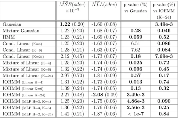
In table 3 and figure 4, the results of experiments on the monthly TSE300 data are presented. Almost all the models (except two of the linear models) are significantly better than the Gaussian for modeling the density of the next month return. The best model is the linear IOHMM, and its performance is significantly better than the performance of the other models. Note also that the models with the 24 inputs (which include not only technical but also economic variables) outperform the models with only technical variables in input.

(16)

0 0.005 0.01 0.015 0.02 0.025 -0.025 -0.02 -0.015 -0.01 -0.005 0 0.005 0.01 0.015 0.02 0.025 Density probabilities TSE300 log-returns Density fonction for a Gaussian (5-day)

0 0.005 0.01 0.015 0.02 0.025 0.03 -0.025 -0.02 -0.015 -0.01 -0.005 0 0.005 0.01 0.015 0.02 0.025 Density probabilities TSE300 log-returns Density fonction for an IOHMM-Linear (5-day)

0 0.005 0.01 0.015 0.02 0.025 -0.025 -0.02 -0.015 -0.01 -0.005 0 0.005 0.01 0.015 0.02 0.025 Density probabilities TSE300 log-returns Density fonction for an IOHMM-MLP (5-day)

Figure 2: Comparison of the shape of the conditional densities predicted for the same time step (out-of-sample) for three models of the 5-day TSE300 log-returns: Gaussian (left), linear IOHMM (middle), non-linear IOHMM (right). The vertical bars show a 90% confidence interval around the expected return.

(17)

2.8 2.9 3.0 3.1 3.2 Log-likelihood

0.0 0.001 0.002 0.003 0.004 0.005

Figure 3: Comparative results on modeling the conditional density of the next TSE300 12-month returns every 12-month. Top: out-of-sample log-likelihood. Bottom: p-value vs MLP IOHMM.

(18)

1.6 1.7 1.8 1.9 2.0 2.1 Log-likelihood

0.0

0.2

0.4

0.6

0.8

p-value (%) vs best model (Linear IOHMM)

Figure 4: Comparative results on modeling the conditional density of the next TSE300 1-month returns every 1-month. Top: out-of-sample log-likelihood. Bottom: p-value vs Linear IOHMM (K = 24).

(19)

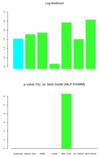
1.1 1.2 1.3 1.4 1.5 1.6 1.7 Log-likelihood

0 1 2 3 4 5 6

Figure 5: Comparative results on jointly modeling the conditional density of the next TSE 14 sectors 1-month returns every month. Top: out-of-sample log-likelihood. Bottom: p-value vs MLP IOHMM (K = 24).

(20)

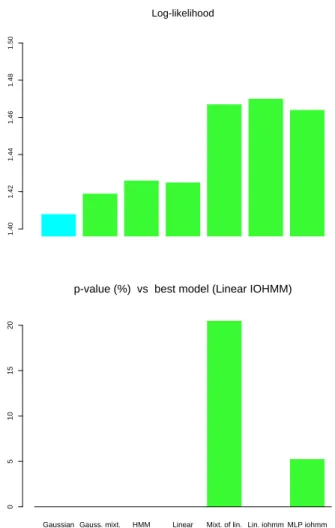
1.40 1.42 1.44 1.46 1.48 1.50 Log-likelihood

0

5

10

15

20

p-value (%) vs best model (Linear IOHMM)

Figure 6: Comparative results on separately modeling the conditional density of the next TSE 14 sectors 1-month returns every month. Top: out-of-sample log-likelihood. Bottom: p-value vs Linear IOHMM (K = 6).

(21)

d

M SE(sdev) N LL(sdev)d p-value (%) p-value(%)

×10−3 _{vs Gaussian} _{vs IOHMM} (K=24) Gaussian 1.22 (0.20) -1.60 (0.08) 3.49e-3 Mixture Gaussian 1.22 (0.20) -1.68 (0.07) 0.28 0.046 HMM 1.23 (0.21) -1.69 (0.07) 0.059 0.52 Cond. Linear(K=4) 1.25 (0.20) -1.63 (0.07) 6.51 0.086 Cond. Linear(K=6) 1.28 (0.21) -1.63 (0.07) 7.62 0.084

Cond. Linear(K=24) 2.12 (0.45) -1.73 (0.07) 0.18 7.69e-3

Mixture of Linear(K=4) 1.25 (0.20) -1.74 (0.06) 0.025 0.72

IOHMM(Linear K=4) 1.31 (0.22) -1.73 (0.06) 0.013 0.74

IOHMM(Linear K=6) 1.39 (0.24) -1.74 (0.05) 0.13 0.32

IOHMM(Linear K=24) 2.27 (0.48) -2.08 (0.09) 3.49e-3

IOHMM(MLP H=3, K=4) 1.25 (0.20) -1.75 (0.06) 4.86e-3 0.090

IOHMM(MLP H=3, K=6) 1.36 (0.22) -1.76 (0.06) 2.56e-3 0.25

IOHMM(MLP H=2, K=24) 1.42 (0.21) -1.87 (0.06) < 1e-7 0.84

Table 3: Results on modeling the next TSE300 1-month returns. Bold MSE or NLL shows the best value obtained. Bold p-values are < 5%, suggesting that the difference with the reference is significant.

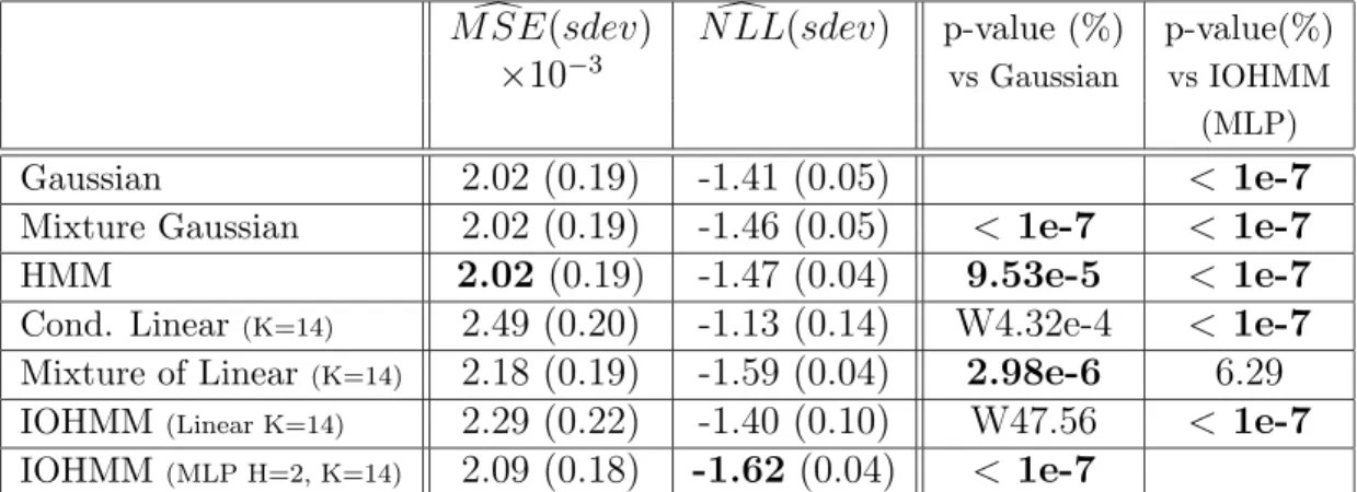
density of the next month’s return for the 14 sector indices. All the conditional models have 14 inputs, for the current return of each of the 14 sectors. The non-linear IOHMM yields the best results, significantly above all the other models except the mixture of linear experts (but the p-value is close to our threshold, at 6.3%). We have also tried to model the relative returns of the sectors with respect to the market index, and the results are shown in table 5. Again, the non-linear IOHMM performed best in NLL, but here the difference with the linear IOHMM is not statistically significant.

In table 6 and figure 6, the results of the other experiments on the monthly 14 sectors of the TSE300 data are presented, where each sector has been trained individually. For predicting the conditional density, the Gaussian is beaten significantly by all the other models. The best-performing model is one of the linear IOHMMs. It outperforms significantly all the models except an IOHMM with MLP (5 hidden units, 1 input) and the mixture of linear experts (with 6 inputs).

5 Conclusions

In this paper we have applied Input/Output Hidden Markov Models to financial time-series data in a number of comparative experiments aimed at measuring the expected generalization

(22)

d

×10−3 _{vs Gaussian} _{vs IOHMM}

(MLP)

Gaussian 2.02 (0.19) -1.41 (0.05) < 1e-7

Mixture Gaussian 2.02 (0.19) -1.46 (0.05) < 1e-7 < 1e-7

HMM 2.02 (0.19) -1.47 (0.04) 9.53e-5 < 1e-7

Cond. Linear(K=14) 2.49 (0.20) -1.13 (0.14) W4.32e-4 < 1e-7

Mixture of Linear(K=14) 2.18 (0.19) -1.59 (0.04) 2.98e-6 6.29

IOHMM(Linear K=14) 2.29 (0.22) -1.40 (0.10) W47.56 < 1e-7

IOHMM(MLP H=2, K=14) 2.09 (0.18) -1.62 (0.04) < 1e-7

Table 4: Results on jointly modeling the next 14 sectors 1-month returns (one model used for all the sectors). Bold MSE or NLL shows the best value obtained. Bold p-values are < 5%, suggesting that the difference with the reference is significant.

error of different types of model structures. The main conclusions from the experiments are the following:

• For predicting the expected future returns, none of the models we have tried performs better than the simple-minded historical average, i.e., we get better predictions of the mean using an unconditional model.

• For predicting the future distribution of the returns at a fixed horizon, we have found IOHMMs to perform significantly better than other models, more specifically:

– For predicting the next 5-day return of the TSE300, the non-linear IOHMM (with MLPs) is significantly better than all the other models.

– For predicting the next 12-month return of the TSE300, the non-linear IOHMM (with MLPs) is significantly better than all the other tested models.

– For predicting the next 1-month return of the TSE300, the linear IOHMM with fundamental economic input variables is significantly better than all the other models.

– For predicting the next 1-month return of the 14 sector indices,

∗ when predicting all 14 sectors simultaneously, the non-linear IOHMM (with MLPs) is significantly better than all the other tested models (except the mixture of linear experts, against which the p-value is 6.3%).

∗ when predicting all 14 sectors simultaneously, one of the linear IOHMMs is significantly better than most other models except a non-linear IOHMM and a mixture of linear experts.

By looking over these results and trying to answer qualitative questions about which type of models make better predictions, we find that the results broadly suggest that for predicting

(23)

d

×10−3 _{vs Gaussian} _{vs IOHMM}

(MLP)

Gaussian 0.994 (0.071) -1.81 (0.036) 3.0e-6

Mixture Gaussian 0.994 (0.071) -1.81 (0.036) 1.46e-4 3.0e-6

HMM 0.994 (0.071) -1.81 (0.036) 9,96e-1 3.0e-6

Cond. Linear(K=14) 1.14 (0.083) -1.82 (0.035) 41.13 < 1e-7

Mixture of Linear (K=14) 1.14 (0.083) -1.87 (0.025) 9.73e-3 1.32

IOHMM (Linear K=14) 1.23 (0.088) -1.89 (0.026) 7.44e-1 47.29

IOHMM (MLP H=2, K=14) 1.05 (0.077) -1.89 (0.029) 2.98e-6

Table 5: Results on jointly modeling the next 14 sectors 1-month relative returns (with respect to the TSE300 index). Bold MSE or NLL shows the best value obtained. Bold p-values are < 5%, suggesting that the difference with the reference is significant.

the density of the next returns or relative returns, (1) conditional models perform better, (2) using a state variable that can deal with regime changes yields better performance, (3) combining both conditional predictions and a state variable yields even better results, and in most cases (4) non-linear predictions associated to each state yield even better results than linear predictions.

There are many more experiments and analyses that should be done in order to pur-sue in the direction explored here. Most interestingly, we would like to ascertain whether the improvements in likelihood brought by the various mixture models, and in particular the IOHMMs, can be used in order to improve financial decision-taking, e.g., for assessing risk in portfolio management or for trading options. Also, in view of the fact that the model is good at predicting higher moments, it would be interesting to apply it as a risk-assessing tool (for example to evaluate value-at-risk) rather than as a tool to predict expected returns. It might be used as such (for controlling risk), or incorporated in a system that trades on predictions of volatility. Another type of application of the IOHMM is as a generative model for para-metric bootstrap. The IOHMM could thus be used to generate many alternative plausible histories, over which the variability of any learning algorithm (for example the variability of its out-of-sample performance) could be assessed.

References

Baldi, P. and Brunak, S. (1998). Bioinformatics, the Machine Learning Approach. MIT Press. Baldi, P., Chauvin, Y., Hunkapiller, T., and McClure, M. (1995). Hidden markov models of biological primary sequence information. Proc. Nat. Acad. Sci. (USA), 91(3):1059–1063. Bengio, S. and Bengio, Y. (1996). An EM algorithm for asynchronous input/output hidden

(24)

d

M SE(sdev) N LL(sdev)d p-value (%) vs p-value(%) vs

×10−3 _Gaussian _{Lin. IOHMM}

(K=6)

Gaussian 2.017 (.080) -1.408 (.019) < 1e-7

Mixture Gaussian 2.017 (.080) -1.419 (.018) 2.53e-4 < 1e-7

HMM 2.017 (.080) -1.426 (.018) 7.74e-5 < 1e-7

Cond. Linear (K=1) 2.013 (.081) -1.417 (.018) 0.31 < 1e-7

Cond. Linear (K=2) 2.030 (.081) -1.421 (.018) 0.17 < 1e-7

Cond. Linear (K=4) 2.049 (.082) -1.425 (.018) 0.073 < 1e-7

Cond. Linear (K=6) 2.064 (.083) -1.423 (.018) 0.097 < 1e-7

Mixture of Linear (K=1) 2.014 (.080) -1.430 (.018) 5.96e-6 < 1e-7

Mixture of Linear (K=2) 2.030 (.081) -1.436 (.018) 5.96e-6 < 1e-7

Mixture of Linear (K=4) 2.048 (.081) -1.458 (.016) < 1e-7 0.024

Mixture of Linear (K=6) 2.061 (.082) -1.467 (.016) < 1e-7 20.48

IOHMM (Linear K=1) 2.015 (.081) -1.431 (.018) < 1e-7 < 1e-7

IOHMM (Linear K=2) 2.031 (.081) -1.439 (.018) 5.96e-6 < 1e-7

IOHMM (Linear K=4) 2.050 (.081) -1.461 (.016) < 1e-7 1.06

IOHMM (Linear K=6) 2.073 (.083) -1.470 (.016) < 1e-7

IOHMM (MLP H=5, K=1) 2.022 (.080) -1.464 (.017) < 1e-7 5.26

IOHMM (MLP H=5, K=2) 2.051 (.081) -1.446 (.016) < 1e-7 8.94e-6

IOHMM (MLP H=3, K=4) 2.032 (.079) -1.445 (.017) < 1e-7 2.68e-5

IOHMM (MLP H=2, K=6) 2.035 (.081) -1.443 (.017) < 1e-7 < 1e-7

Table 6: Results on modeling the TSE300 14 sectors (1-month) returns, with a separate model for each sector. Bold MSE or NLL shows the best value obtained. Bold p-values are < 5%, suggesting that the difference with the reference is significant.

Markov models. In Xu, L., editor, International Conference On Neural Information Processing, pages 328–334, Hong-Kong.

Bengio, Y. (1996). Markovian models for sequential data. Technical Report 1049, Dept. IRO, Universit´e de Montr´eal.

Bengio, Y. and Frasconi, P. (1995). An input/output HMM architecture. In Tesauro, G., Touretzky, D., and Leen, T., editors, Advances in Neural Information Processing Systems 7, pages 427–434. MIT Press, Cambridge, MA.

Bengio, Y. and Frasconi, P. (1996). Input/Output HMMs for sequence processing. IEEE Transactions on Neural Networks, 7(5):1231–1249.

Bengio, Y., LeCun, Y., Nohl, C., and Burges, C. (1995). Lerec: A NN/HMM hybrid for on-line handwriting recognition. Neural Computation, 7(5):1289–1303.

(25)

Bramson, M. and Hoptroff, R. (1990). Forecasting the economic cycle: a neural network approach. In Workshop on Neural Networks for Statistical and Economic Data, Dublin. Cacciatore, T. W. and Nowlan, S. J. (1994). Mixtures of controllers for jump linear and non-linear plants. In Cowan, J., Tesauro, G., and Alspector, J., editors, Advances in Neural Information Processing Systems 6, San Mateo, CA. Morgan Kaufmann.

Chauvin, Y. and Baldi, P. (1995). Hidden markov models of the g-protein-coupled receptor family. Journal of Computational Biology.

Dempster, A. P., Laird, N. M., and Rubin, D. B. (1977). Maximum-likelihood from incomplete data via the EM algorithm. Journal of Royal Statistical Society B, 39:1–38.

Diebold, F., Lee, J., and Weinbach, G. (1993). Regime switching with time-varying transi-tion probabilities. In Hargreaves, C., editor, Nonstatransi-tionary Time Series Analysis and Cointegration. Oxford University Press, Oxford.

Garcia, R. (1995). Asymptotic null distribution of the likelihood ratio test in markov switching models. Technical Report 95s-7, CIRANO, Montreal, Quebec, Canada.

Garcia, R. and Perron, P. (1995). An analysis of the real interest rate under regime shift. Technical Report 95s-5, CIRANO, Montreal, Quebec, Canada.

Garcia, R. and Schaller, H. (1995). Are the effects of monetary policy asymmetric. Technical Report 95s-6, CIRANO, Montreal, Quebec, Canada.

Ha, J., Oh, S., Kim, J., and Kwon, Y. (1993). Unconstrained handwritten word recogni-tion with interconnected hidden Markov models. In Third Internarecogni-tional Workshop on Frontiers in Handwriting Recognition, pages 455–460, Buffalo. IAPR.

Hamilton, J. (1988). Rational-expectations econometric analysis of changes in regime. Jour-nal of Economic Dynamics and Control, 12:385–423.

Hamilton, J. (1989). A new approach to the economic analysis of non-stationary time series and the business cycle. Econometrica, 57(2):357–384.

Hamilton, J. (1996). Specification testing in markov-switching time-series models. Journal of Econometrics, 70:127–157.

Jacobs, R. A., Jordan, M. I., Nowlan, S. J., and Hinton, G. E. (1991). Adaptive mixture of local experts. Neural Computation, 3:79–87.

Karplus, K., Sjolander, K., Barrett, C., Cline, M., Haussler, D., Hughey, R., Holm, L., and Sander, C. (1997). Predicting protein structure using hidden markov models. Proteins: Structure, Function and Genetics, Supp. 1(1):134–139.

Krogh, A., Brown, M., Mian, I., Sj¨olander, K., and Haussler, D. (1994). Hidden markov models in computational biology: Applications to protein modeling. Journal Molecular Biology, 235:1501–1531.

(26)

Krolzig, H.-M. (1997). Markov-Switching Vector Autoregressions. Springer.

Kundu, A. and Bahl, L. (1988). Recognition of handwritten script: a hidden Markov model based approach. In International Conference on Acoustics, Speech and Signal Processing, pages 928–931, New York, NY.

Lauzon, V.-P. (1999). Modèles statistiques comme algorithmes d’apprentissage et MMCCs; prédiction de séries financières. Master’s thesis, Département d’informatique et recherche opérationnelle, Université de Montréal, Montréal, Québec, Canada.

Matan, O., Burges, C., LeCun, Y., and Denker, J. (1992). Multi-digit recognition using a space displacement neural network. In Moody, J., Hanson, S., and Lipmann, R., editors, Advances in Neural Information Processing Systems 4, pages 488–495, San Mateo CA. Morgan Kaufmann.

Moody, J. (1998). Forecasting the economy with neural nets: a survey of challenges. In Orr, G. and Muller, K.-R., editors, Neural Networks: Tricks of he Trade, pages 347–372. Springer.

Moody, J., Levin, U., and Rehfuss, S. (1993). Predicting the U.S. index of industrial produc-tion. Neural Network World, 3(6):791–794.

Nag, R., Wong, K., and Fallside, F. (1986). Script recognition using hidden Markov models. In International Conference on Acoustics, Speech and Signal Processing, pages 2071–2074, Tokyo.

Schenkel, M., Guyon, I., and Henderson, D. (1995). On-line cursive script recognition using time delay neural networks and hidden Markov models. Machine Vision and Applica-tions, pages 215–223.

Schenkel, M., Weissman, H., Guyon, I., Nohl, C., and Henderson, D. (1993). Recognition-based segmentation of on-line hand-printed words. In Hanson, S. J., Cowan, J. D., and Giles, C. L., editors, Advances in Neural Information Processing Systems 5, pages 723– 730, Denver, CO.

Smyth, P. (1994). Hidden markov models for fault detection in dynamic systems. Pattern Recognition, 27(1):149–164.

Sola, M. and Driffill, J. (1994). Testing the term structure of interest rates using a station-ary vector autoregression with regime switching. Journal of Economic Dynamics and Control, 18:601–628.

Viterbi, A. (1967). Error bounds for convolutional codes and an asymptotically optimum decoding algorithm. IEEE Transactions on Information Theory, pages 260–269.

(27)

Liste des publications au CIRANO*

Série Scientifique / Scientific Series (ISSN 1198-8177)

2002s-48 Experiments on the Application of IOHMMs to Model Financial Returns Series / Y. Bengio, V.-P. Lauzon et R. Ducharme

2002s-47 Valorisation d'options par optimisation du Sharpe Ratio / Y. Bengio, R. Ducharme, O. Bardou et N. Chapados

2002s-46 Incorporating Second-Order Functional Knowledge for Better Option Pricing / C. Dugas, Y. Bengio, F. Bélisle, C. Nadeau et R. Garcia

2002s-45 Étude du biais dans le prix des options / C. Dugas et Y. Bengio 2002s-44 Régularisation du prix des option : Stacking / O. Bardou et Y. Bengio

2002s-43 Monotonicity and Bounds for Cost Shares under the Path Serial Rule / Michel Truchon et Cyril Téjédo

2002s-42 Maximal Decompositions of Cost Games into Specific and Joint Costs / Michel Moreaux et Michel Truchon

2002s-41 Maximum Likelihood and the Bootstrap for Nonlinear Dynamic Models / Sílvia Gonçalves et Halbert White

2002s-40 Selective Penalization Of Polluters: An Inf-Convolution Approach / Ngo Van Long et Antoine Soubeyran

2002s-39 On the Mediational Role of Feelings of Self-Determination in the Workplace: Further Evidence and Generalization / Marc R. Blais et Nathalie M. Brière 2002s-38 The Interaction Between Global Task Motivation and the Motivational Function

of Events on Self-Regulation: Is Sauce for the Goose, Sauce for the Gander? / Marc R. Blais et Ursula Hess

2002s-37 Static Versus Dynamic Structural Models of Depression: The Case of the CES-D / Andrea S. Riddle, Marc R. Blais et Ursula Hess

2002s-36 A Multi-Group Investigation of the CES-D's Measurement Structure Across Adolescents, Young Adults and Middle-Aged Adults / Andrea S. Riddle, Marc R. Blais et Ursula Hess

2002s-35 Comparative Advantage, Learning, and Sectoral Wage Determination / Robert Gibbons, Lawrence F. Katz, Thomas Lemieux et Daniel Parent

2002s-34 European Economic Integration and the Labour Compact, 1850-1913 / Michael Huberman et Wayne Lewchuk

2002s-33 Which Volatility Model for Option Valuation? / Peter Christoffersen et Kris Jacobs 2002s-32 Production Technology, Information Technology, and Vertical Integration under

Asymmetric Information / Gamal Atallah

2002s-31 Dynamique Motivationnelle de l’Épuisement et du Bien-être chez des Enseignants Africains / Manon Levesque, Marc R. Blais, Ursula Hess

* Consultez la liste complète des publications du CIRANO et les publications elles-mêmes sur notre site Internet :

(28)

2002s-30 Motivation, Comportements Organisationnels Discrétionnaires et Bien-être en Milieu Africain : Quand le Devoir Oblige / Manon Levesque, Marc R. Blais et Ursula Hess 2002s-29 Tax Incentives and Fertility in Canada: Permanent vs. Transitory Effects / Daniel

Parent et Ling Wang

2002s-28 The Causal Effect of High School Employment on Educational Attainment in Canada / Daniel Parent

2002s-27 Employer-Supported Training in Canada and Its Impact on Mobility and Wages / Daniel Parent

2002s-26 Restructuring and Economic Performance: The Experience of the Tunisian Economy / Sofiane Ghali and Pierre Mohnen

2002s-25 What Type of Enterprise Forges Close Links With Universities and Government Labs? Evidence From CIS 2 / Pierre Mohnen et Cathy Hoareau

2002s-24 Environmental Performance of Canadian Pulp and Paper Plants : Why Some Do Well and Others Do Not ? / Julie Doonan, Paul Lanoie et Benoit Laplante

2002s-23 A Rule-driven Approach for Defining the Behavior of Negotiating Software Agents / Morad Benyoucef, Hakim Alj, Kim Levy et Rudolf K. Keller

2002s-22 Occupational Gender Segregation and Women’s Wages in Canada: An Historical Perspective / Nicole M. Fortin et Michael Huberman

2002s-21 Information Content of Volatility Forecasts at Medium-term Horizons / John W. Galbraith et Turgut Kisinbay

2002s-20 Earnings Dispersion, Risk Aversion and Education / Christian Belzil et Jörgen Hansen 2002s-19 Unobserved Ability and the Return to Schooling / Christian Belzil et Jörgen Hansen 2002s-18 Auditing Policies and Information Systems in Principal-Agent Analysis /

Marie-Cécile Fagart et Bernard Sinclair-Desgagné

2002s-17 The Choice of Instruments for Environmental Policy: Liability or Regulation? / Marcel Boyer, Donatella Porrini

2002s-16 Asymmetric Information and Product Differentiation / Marcel Boyer, Philippe Mahenc et Michel Moreaux

2002s-15 Entry Preventing Locations Under Incomplete Information / Marcel Boyer, Philippe Mahenc et Michel Moreaux

2002s-14 On the Relationship Between Financial Status and Investment in Technological Flexibility / Marcel Boyer, Armel Jacques et Michel Moreaux

2002s-13 Modeling the Choice Between Regulation and Liability in Terms of Social Welfare / Marcel Boyer et Donatella Porrini

2002s-12 Observation, Flexibilité et Structures Technologiques des Industries / Marcel Boyer, Armel Jacques et Michel Moreaux

2002s-11 Idiosyncratic Consumption Risk and the Cross-Section of Asset Returns / Kris Jacobs et Kevin Q. Wang

2002s-10 The Demand for the Arts / Louis Lévy-Garboua et Claude Montmarquette

2002s-09 Relative Wealth, Status Seeking, and Catching Up / Ngo Van Long, Koji Shimomura 2002s-08 The Rate of Risk Aversion May Be Lower Than You Think / Kris Jacobs