Gugl : Department of Economics, University of Victoria, P.O. Box 1700, STN CSC, Victoria, B.C., Canada V8W 2Y2; Tel.: (+1) 250 721-8538
egugl@uvic.ca
Leroux: HEC Montréal and CIRPÉE, 3000 chemin de la Côte-Ste-Catherine, Montréal, QC, Canada H3T 2A7; Tel. : (+1) 514 340-6864
justin.leroux@hec.ca
Gugl thanks Nick Baigent, Craig Brett, Philip Curry, Peter Kennedy, Shelly Lundberg, Hervé Moulin, David Scoones, Paul Schure and Linda Welling for their helpful comments on earlier versions of this paper. We also thank our discussant at the WEAI 84th conference in Vancouver, Jamie Woods for his comments on the current version.
Cahier de recherche/Working Paper 09-38
Share the Gain, Share the Pain? Almost Transferable Utility, Changes
in Production Possibilities, and Bargaining Solutions
Elisabeth Gugl
Justin Leroux
Abstract:
Consider an n-person economy in which efficiency is independent of distribution but the
cardinal properties of the agents’ utility functions precludes transferable utility (a property
we call “Almost TU”). We show that Almost TU is a necessary and sufficient condition for
all agents to either benefit jointly or suffer jointly with any change in production
possibilities under well-behaved generalized utilitarian bargaining solutions (of which the
Nash Bargaining and the utilitarian solutions are special cases). We apply the result to
household decisionmaking in the contex of the Rotten Kid Theorem and in evaluating a
change in family taxation.
Keywords: Axiomatic bargaining, solidarity, transferable utility, familyT-taxation, Rotten
Kid Theorem
1
Introduction
Solidarity is a crucially important consideration whenever individuals coopera-tively decide on how to allocate resources among themselves: an agreement is unlikely to be reached if some are hurt while others bene…t in the event of a fore-seeable shock in the available resources. From a normative standpoint, solidarity is also a chief concern when making policy recommendations, as illustrated by the following slightly modi…ed example found in Nash (1950). Suppose Jack and Bill are siblings and have to share the following items: a book, a whip, a ball, a bat, a box, a pen, a toy, a knife, and a hat. Now suppose the parents take away the whip and the knife and replace them with a bucket and a shovel. It may be a relief for them to know that they will either disappoint both children or delight them both. In other words, the parents may want to make sure that their action does not destabilize their childrens’ bonding by making one child better o¤ and the other worse o¤ and thus giving the impression that parents favor one child over the other. On a larger scale, a government may take a similar stance when it comes to family policies: it may be desirable to know that a change in family policies such as changes in parental leave policies or family taxation, –policies that clearly change a family’s production possibility set – do not leave some family members worse o¤ and others better o¤, which could unduly stress intrafamily relationships.
In practice, however, most bargaining situations which draw upon the results of axiomatic bargaining typically do so using some generalized utilitarian bar-gaining solution (GUBS). This broad class of solutions consists of maximizing an additively separable social welfare function and includes the utilitarian and Nash bargaining solutions. Despite their appealing properties (Moulin 1988), bargaining solutions in the GUBS class typically fail to satisfy solidarity (Chun and Thomson, 1988) unless agents’ utility is transferable. Yet, transferable utility (TU) is a very strong assumption which forbids taking into account com-monly observed features of individual preferences such as diminishing marginal utility and, by extension, risk aversion. Hence, for most practical purposes, the use of the class of GUBS seems rather limited in applications.
We remedy the issue by establishing that well-behaved GUBS (to be de…ned) satisfy solidarity on a broader utility class than TU, which we de…ne and call Almost TU. Almost TU requires the same ordinal properties as TU but allows for cardinal properties like diminishing marginal utility as well. Hence, our result broadens the valid range of applications for bargaining solutions of the GUBS class.1 Also, from an implementation standpoint, policy makers may be unsure of the cardinal properties of agents’ utility functions when evaluating the change in welfare due to a change in policy. Hence they may be reassured to know that the utility of the agents will change in the same direction even in the event of a misestimation of these cardinal properties, as long as the ordinal
1MasCollel et al. (1995, p. 831) take as given that individuals have cardinal utility
func-tions, when they state:"[...] whereas a policy maker may be able to identify individual cardinal utility functions (from revealed risk behavior, say), it may actually do so but only up to a choice of origins and units."
properties for TU are satis…ed.
More precisely, our main result (Theorem 1) characterizes Almost TU as the domain on which all well-behaved GUBS satisfy solidarity. We then present two applications where our main result bears useful consequences. First, in family policies, changes in family taxation amount to changes in the production possi-bility set of the household. Consquently, knowing that the solidarity property holds helps decrease the number of dimensions of possible opposition to a policy change (i.e., only interhousehold tensions will have to be considered, but not intrahousehold tensions). The second application we o¤er relates to the ques-tion of incentive compatibility (Theorem 2) and as an applicaques-tion we present a version of the Rotten Kid Theorem which holds on the wider domain of Almost TU instead of TU.
Even if a GUBS satis…es the solidarity property, there is still a possibility that a change in the utility possibility set a¤ects agents’ utilities in opposite ways. This happens if not only joint production possibilities change but the stand-alone utilities of agents change as well (see section 6 for examples). Yet, even in this case, Almost TU in combination with a GUBS remains useful as it allows us to decompose the impact of such a change into a "utility possibility set" e¤ect (agents share the gain or the pain holding the disagreement point …xed) and a "disagreement point" e¤ect (di¤erent agents may experience changes in their utility at the disagreement point in opposing directions).
2
Related Literature
Many works emphasize the importance of solidarity in allocation problems, be it with respect to population or to the total amount of goods available (see Moulin, 1988, or Sprumont, 2008, for a survey.) This work belongs to the latter strand of the literature and is more closely related to Chun and Thomson (1988), which explicits the parallel between fair allocation problems and bargaining situations. Chun and Thomson (1988) show that the solidarity property holds in a one-good economy for some bargaining solutions. Our main result generalizes theirs to a many-goods production economy when preferences exhibit Almost TU.
In the context of axiomatic bargaining, many characterizations of bargaining solutions are motivated by at least some notion of solidarity or monotonicity arguments.2 Xu and Yoshihara (2008) o¤er a systematic treatment of well-known bargaining rules with respect to solidarity-type axioms.
Although we motivate the interest in the solidarity property as a normative issue, our result also has implications for incentive compatibility. In an applica-tion of our main theorem we draw a connecapplica-tion to Bergstrom’s (1989) treatment of the Rotten Kid Theorem.3 Bergstrom shows that each child behaves so as to
2Individual monotonicity is the property that distinguishes the Kalai-Smorodinsky solution
from the Nash Bargaining solution (Kalai and Smorodinsky 1975).
3There has been renewed interest in the Rotten Kid Theorem in explaining the economics
of child labor (Baland and Robinson 2000, and Bommier and Dubois 2004). The question of whether or not TU is a reasonable assumption in this context plays a crucial role in these two
maximize the head of household’s altruistic utility function if and only if util-ity is transferable. By strengthening the assumption on the altruistic parent’s preferences to be of the form of a well-behaved GUBS rather than just treating each child as a normal good, we present a Rotten Kid Theorem that holds for Almost TU, not just TU.
The issue of incentive compatibility also arises in a model in which spouses need to take individual actions in order to produce goods that they will later distribute among themselves. Based on Gugl (2009) we provide such a model of "Rotten Spouses" in section 6.1. Almost TU takes care of two issues at once: Assuming Almost TU, the class of well-behaved GUBS satis…es the Solidarity property as well as incentive compatibility.
3
The Model
Consider a population N = f1; 2; :::; ng of agents who produce L 2 goods. These goods may include public goods, but at least one good is private. More precisely, the population faces a production possibility set Y RL
+ that is a closed, convex and comprehensive set. If we denote by y 2 RL
+ a particular product mix, then @Y , the production possibility frontier of Y , and the corre-sponding transformation function, F : RL+! R, are de…ned as follows:
Y = y 2 RL+jF (y) 0 , and @Y = fy 2 Y jF (y) = 0g :
We denote by xi = (xi1; xi2; :::; xiL) 2 RL+ agent i’s consumption vector. A distribution of y is a list of consumption vectors, one per agent, x = (x1; :::; xn) such that:
P
i2Nxil= yl for any private good, l, and xik= xjk = yk for all i; j 2 N and any public good, k:
For any product mix y, we denote by X(y) the set of distributions of y and by X(Y ) =Sy2Y X(y) the set of feasible distributions under Y . An allocation is a product mix-distribution pair (y; x) 2 Y X(y):
The preferences of each agent i are represented by a utility function, ui, which is non-decreasing, concave and twice di¤erentiable from RL
+ to R.4 We denote by U the class of such utility functions. A utility pro…le is a collection of utility functions, (u1; u2; :::; un) 2 UN, one per agent. An economy is a pair (Y; u) 2 RL
+ UN.
We denote by U (Y; u) = f 2 RNj9x 2 X(Y ) s.t. u(x) = g the utility possibility set corresponding to the economy (Y; u). It follows from our assump-tions on an economy that U (Y ) is a closed, convex, and comprehensive set.
papers.
4We assume di¤erentiability for expositional purposes, but our results extend to
We denote by @U (Y; u) the Pareto frontier of U (Y; u); i.e., @U (Y; u) = f 2 U (Y; u)j 0 =) 02 U(Y; u)g.= 5
We shall consider that agents cooperatively manage the economy, in the form of a bargaining process, with the possibility that agents disagree on how to do so. Hence, we denote by di agent i’s stand-alone utility level and call d = (d1; d2; :::; dn) 2 U(Y; u) the disagreement point of the bargaining process. We denote by the pair (U (Y; u); d) the corresponding bargaining problem. Note that we take the view that the disagreement point may depend on the utility pro…le, u, but is independent of the cooperative production possibilities, Y .
A bargaining solution is a function, S : RL
+ UN RN ! U(Y; u), map-ping to each bargaining problem a utility vector in the corresponding utility possibility set such that S(U (Y; u); d)= d and S(U(Y; u); d) 2 @U (Y; u). We denote by S the class of bargaining solutions. A family of bargaining solu-tions we shall consider is that of generalized utilitarian bargaining solusolu-tions (GUBS) where, for each bargaining solution in this class, there exists a list of n concave, strictly increasing, and continuous functions, ( 1; 2; ::: n), such that (U (Y; u); d) = arg max 2@U(Y;u)Pi2N i( i di). Note that GUBS is a wide family of bargaining solutions; both the utilitarian solution and the Nash bargaining solution belong to GUBS, with i= 1 and i= ln( ) for all i, respec-tively. More precisely, we denote by G the subclass of GUBS for which the i’s are strictly concave; thus, so the Nash Bargaining solution belongs to G. The utilitarian solution belongs to another subclass of GUBS, the weighted utilitar-ian bargaining solutions (WUBS): A bargaining solution W belonging to WUBS is characterized by a list of n non-negative weights, (!1; !2; :::; !n) 2 RN+, with P
!i = 1, such that W (U (Y; u); d) 2 arg max 2@U(Y;u)Pi2N!i( i di). To ensure uniqueness of the solution in case @U (Y; u) is an (n 1)-dimensional hyperplane as Pareto frontier, we shall consider only the subfamily of WUBS which break ties along a non-decreasing path of RN
+: A non-decreasing path is a function : R+ ! RN+ s.t. (t) = ( 1(t); 2(t); :::; n(t)) non-decreasing in each coordinate with (0) = d andPi i(t) = t +Pidi.
W (U (Y; u); d) = arg min 2arg max 2@U(Y;u)
P !i( i di) max 2@U(Y;u) X !i( i di)
By convexity of U (Y; u), W (U (Y; u); d) is unique. We denote by W the family of WUBS breaking ties along a non-decreasing path. We refer to a G [ W as the class of well-behaved GUBS.
We say that a bargaining solution, S, satis…es Solidarity under utility pro…le u if one of the following vector inequality holds:
S(U (Y; u); d)= S(U(Y0; u); d) or S(U (Y; u); d)5 S(U(Y0; u); d) for any Y; Y0 RL
+, and any d 2 RN+.
5We adopt the ususal notational convention for vector inequalities: x= x0, x x0, and
4
Almost Transferable Utility
In this section we de…ne the new concept of Almost Transferable Utility. In order to do so, we …rst recall what is meant by a product mix that being e¢ cient independently of distribution, a necessary (and su¢ cient) condition for (Almost) TU to hold. The conditions under which a product mix is e¢ cent independently of distribution are well established in the literature by Bergstrom and Cornes (1983) and Bergstrom and Varian (1985). Our analysis below is not meant to reestablish these results but to apply the concept to introduce Almost TU.
4.1
E¢ ciency Independent of Distribution
6We denote by EX(y; u) = fx 2 X(y)j@x0 2 X(y); u(x0) u(x)g the set of exchange e¢ cient distributions in X(y) relative to the utility pro…le u and by P (Y; u) = f(y; x) 2 Y X(y)j@(y0; x0) 2 Y X(y0); u(x0) u(x)g the set of (Pareto) e¢ cient allocations in the economy (Y; u).
For any given y 2 Y , we say that x 2 X (y) is interior exchange e¢ cient if and only if:
@ui(xi) @xli @ui(xi) @xmi = @uj (xj ) @xlj @uj (xj ) @xmj
for all i; j 2 N, for all private goods l; m:
We denote by EX (y; u) the set of interior exchange e¢ cient distributions of X(y) relative to the utility pro…le u: We say that a product mix and distribution pair (y; x) 2 Y X(y) is interior e¢ cient if and only if the following holds: 8 > > < > > : @ui(xi) @xli @ui(xi) @xmi = @F (y) @yl @F (y)
@ym for all i 2 N, and all private goods l; m
and Pi2N @ui(xi) @xk @ui(xi) @xmi = @F (y) @yk @F (y) @ym
for any public good k and any private good m. (1) The …rst family of equalities states that all agents’ marginal rates of substi-tutions (MRS) between any two private goods, @ui(xi)
@xli =
@ui(xi)
@xmi ; must equal the
marginal rate of transformation (MRT) between these goods, @F (y)@x
l =
@F (y) @xm . The
second set of equalities are the Samuelson conditions for public goods.
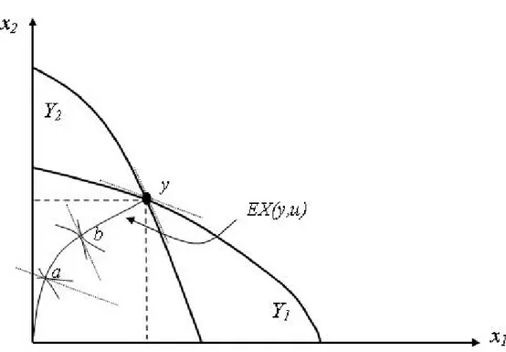
We say that e¢ ciency is independent of distribution if there exists y 2 Y such that, for all 2 @U (Y; u), = u (x) for some x 2 X (y) : In words, all points on the utility possibility frontier are be achieved via vasiour distributions of the same product mix. It follows from (1) that y is associated with a vector of marginal rates of substitution at the exchange e¢ cient distributions— one per pair of goods— which is independent of the utility level achieved by any agent. See Figure 1 for a graphical illustration in the case of two private goods, strictly quasi-concave utility functions and a strictly convex production possibility set.
6Bergstrom and Cornes (1983) call this concept "independence of allocative e¢ ciency from
In the …gure, neither y nor y0 are e¢ cient, because the value of the MRS as-sociated with EX (y; u) is di¤erent from the MRT at y; similarly for y0. The product mix associated with any e¢ cient allocation, y00, lies on @Y between y and y0, where the MRS of EX (y00; u) equals the MRT at y00.
Figure 1: E¤…cicency independent of distribution: Anll e¢ cient distributions aggregate up to the same product mix y00:
In the case of public and private goods, for a product mix to be e¢ cient independently of distribution requires that the sum of marginal rates of substi-tution stays the same for a given level of the public good yk no matter how the total amount of the private good ylis distributed.
4.2
Transferable Utility
A utility pro…le, u 2 UN, satis…es Transferable Utility (Bergstrom 1989) if for any given Y 2 RL
+, the following holds:
@U (Y; u) = f 2 U(Y; u) :X i2N
Note that resource and technological constraints as given by Y only play a role in the size of : If TU holds, e¢ ciency is independent of distribution (Bergstrom and Cornes 1983, and Bergstrom and Varian 1985). If we take agents’ utility to be ordinal, the converse is also true. Bergstrom and his co-authors give an exhaustive list of agents’ utility functions that lead to TU. Agents’ utility functions must allow the indirect utility representation of the Gorman Polar Form in an economy with only private goods (Bergstrom and Varian 1985) and a form dual to the Gorman Polar form in an economy with public and private goods (Bergstrom and Cornes 1981 and 1983).
Example 1 Finding the utility possibility frontier with TU.
a) Two private goods, two agents. Suppose ui= (x1ix2i)1=2: Then @U (Y; u) = f( 1; 2) 2 U (Y; u) : 1+ 2= (Y; u)g; where = maxy2Y (y1y2)1=2:Indeed, because both agents have identical preferences for any given y 2 Y; dividing all goods equally must be exchange e¢ cient, i.e. x = 12y1;12y2;12y1;12y2 2 EX (y; u) : Therefore (y; u) = 1
2(y1y2) 1=2 +1 2(y1y2) 1=2 = (y1y2)1=2and (Y; u) = maxy2@Y (y1y2)1=2:
b) A private and a public good, two agents. Suppose preferences over a private good and a public good are quasi-linear such that ui = x1i + hi(x2) ; where hi( ) is a strictly concave function. Then the segment of the utility pos-sibility frontier at which TU holds consists of all the points on the line from ( 1= h1(y2) ; 2= y1+ h2(y2)) to ( 1= y1+ h1(y2) ; 2= h2(y2)) where the vector (y1; y2) is found by arg maxy2Y y1+h1(y2)+h2(y2) ; and = maxy2Y y1+ h1(y2) + h2(y2) :
More generally, when TU holds, one can …nd @U (Y; u) in two steps. First, calculate (y; u) =Pi2Nui(xi)such that x 2 EX (y; u) : Second, …nd (Y; u) =
maxy2@Y (y; u) :
4.3
Almost Transferable Utility
Whether a product mix is e¢ cient independently of distribution, depends solely on the ordinal properties of the agents’utility functions. If they are such that a product mix is e¢ cient independently of distribution, but their cardinal prop-erties prohibit the particular utility representation that would lead to TU, then there must exist positive monotonic transformations,fi: R ! R, such that
X i2N
fi( i) = (Y; f (u)) :
However, fi( i) no longer represents an agent’s utility. Hence, we say that pro…le u 2 UN exhibits Almost Transferable Utility (Almost TU) if, for any given Y , the utility possibility frontier is of the form
@U (Y; u) = f 2 U(Y; u) :X i2N
Since ui is assumed to be concave, it follows that fimust be an increasing, and convex function. The intuition is that in order to recover a linear constraint, one needs constant "marginal utility" of money. Hence, given that strict concavity of uileads to decreasing marginal utility of money, a strictly convex transformation is required to undo this e¤ect.
Example 2 Finding the utility possibility frontier with Almost TU.
a) Take the same ordinal properties as in Example 1, but di¤ erent cardinal properties. Suppose u1 = (x11x21)1=3 and u2 = (x12x22)1=4; that is, given u from example 1a), u = u2=31 ; u1=22 : Then @U (Y; u) = f( 1; 2) 2 R2
+ : 3=2 1 + 2 2= Y; u 3=2 1 ; u22 g; where = maxy2Y (y1y2)1=2:
b) Suppose the cardinal utility function of agent i over a private good (x1i) and a public good (x2) is given by ui= (x1i+ hi(x2)) i; where hi( ) is a strictly concave function and i2 (0; 1). Then the segment of the utility possibility
fron-tier at which Almost TU holds consists of the endpoints ( 1= (h1(y2))a1; 2= (y1+ h2(y2)) 2) and ( 1= (y1+ h1(y2)) 1; 2= (h2(y2)) 2) and of all points ( 1; 2) between
these endpoints for which 1= 1
1 + 1= 2 2 = Y; u 1= 1 1 ; u 1= 2
2 ; where the vector (y1; y2) is found by arg maxy2Y y1+ h1(y2) + h1(y2) ; and = maxy2Y y1+ h1(y2) + h1(y2) :
In the following example (Almost) TU does not hold; although there exists a Y such that U (Y; u) forms a simplex, it is not the case for all production possibility sets.
Example 3 Three private goods, two agents. Let u1 and u2 be strictly increas-ing, strictly quasi-concave and homogenous of degree one. Moreover, let u1 = u (x11; x21) ; u2= u (x12; x32) : That is, good 3 replaces good 2 in agent’s 2 utility function as compared to that of agent 1’s. Let (Y; u1) = maxy2Y u (x11; x21) and (Y; u2) = maxy2Y u (x12; x32) : Consider the production possibility set given by Y = (y1; y2; y3) 2 R3+jy1+ p2y2+ p3y3 I with p2; p3; I > 0 and p2 = p3 = p: Then, (Y; u1) = (Y; u2) and @U (Y; u) = f( 1; 2) 2 U (Y; u) : 1+ 2 = (Y; u1) = (Y; u2)g: Suppose Y changes to Y0 such that Y0 = (y1; y2; y3) 2 R3+jy1+ p2y2+ p3y3 I with p26= p3: Then @U (Y0; u) = f( 1; 2) 2 U (Y0; u) : 1
(Y0;u1)+ (Y02;u2) = 1g: (Almost) TU is violated. Proof see Appendix.
5
Results
We now consider what happens if Almost TU holds and the production possi-bility set changes.
Lemma Given Almost TU, a change in the production possibilities of the econ-omy can only result in an expansion or a contraction of the utility possi-bility set:8Y; Y02 RL
Proof. Consider a change from Y to Y0: By Almost TU, @U (Y; u) = f 2 U (Y; u) :Pfi( i) = (Y; f (u))g and @U(Y0; u) = f 2 U(Y0; u) :
P
fi( i) = (Y0; f (u))g. Hence, either (Y; f (u)) = (Y0; f (u)), in which case U (Y; u) = U (Y0; u) ; or (Y; f (u)) > (Y0; f (u)) implying U (Y; u) U (Y0; u) ; or (Y; f (u)) <
(Y0; f (u)) implying U (Y; u) U (Y0; u) : We now state our main theorem.
Theorem 1 Any bargaining solution, S 2 G [ W, satis…es solidarity under pro…le u if and only if u exhibits Almost TU.
Proof. For su¢ ciency, note that for any S 2 G [ W, a …rst step— and, in case of S 2 G, also the last step— to …nding S is by solving the following:
max Pi2N i( i di) s:t: Pi2Nfi( i) = (Y; f (u))
(2)
In what follows, it will be useful to work with vi= fi( i), such that the above problem becomes
max Pi2N i(fi 1(vi) di) s:t: Pi2Nvi= (Y; f (u))
(3)
and then …nding the corresponding i from i = fi 1(vi): Chun and Thomson (1988) show that if agents have concave utility functions over one good only, and this good’s supply increases, both agents bene…t under the Nash bargaining solution. The authors remark that the result extends to any bargaining solution in G (Chun and Thomson 1988, p. 19). When problem (2) is presented as (3) ; a change in (Y; f (u)) due to a change in Y has the same impact on v as a change in the only good has on agents’ utilities in Chun and Thomson (1988)’s one-good economy. Thus their proof applies to our problem (3) for any G2G such that limxi!0gi = 1. In addition, our proof of su¢ ciency below also handles
the subclass W of GUBS, the possibility of corner solutions7,and accounts for d 6= (0; 0) :
Suppose Almost TU holds, and let S 2 G [ W, Y RL
+, u 2 UN and d 2 U(Y; u): Denote by v = S(fv 2 RNjP
i2Nvi (Y; f (u))g; d) the solution vector in the v-space.
Case 1: dfi2
d 2 i(f
1
i (vi)) > 0 for at least n 1 values of i 2 N. It follows that v is the unique element of @f (U (Y; u)) such that the following expression holds: 8 < : @ i @(f 1 i (vi) di) dfi1 dvi (vi) = @ j @(f 1 j (vj) dj) dfj 1 dvj (vj) for all i; j 2 N
such that fi 1(vi) > max i; di and fj 1(vj) > max j; dj ; (4)
7The possibility of corner solutions is not a concern in the proof of Chun and Thomson
where i (resp. j) is the utility level of agent i (resp. agent j) when she does not receive any private good. The left hand side of (4) depends on vi only, and the right hand side of (4) depends on vj only: Since fi 1( ) is increasing and concave, df
1 i
dvi is positive and non-increasing. Similarly, i
being concave and fi 1being increasing, @ i
@(fi1(vi) di) is non-increasing in
vi. Hence, the product @(f 1@ i i (vi) di) df 1 i dvi (resp. @ j @(fj 1(vj) dj) dfj1 dvj ) is
non-increasing in vi (resp.vj). Therefore, for (4) to hold as changes values, vi and vj must change in the same direction, thus proving the result.
Case 2: d2fi
dv2 i (f
1
i (vi)) > 0 for at most n 2 values of i 2 N. If S 2 G, v is the unique element of @f (U (Y; u)) for which expression (4) holds and the argument of Case 1 follows through. Now, suppose S 2 W, with ! 2 Rn
+ its associated weights, there may be more than one v 2 @f(U(Y; u)) for which expression (4) holds. Denote
(Y; u; !) = 8 > > < > > : 2 @U(Y; u)j !i df 1 i @vi (vi) = !j df 1 j dvj (vj) for all i; j 2 N
and i> max i; di and j > max j; dj : 9 > > = > > ; .
We proceed to show that the fact that (Y; u; !) may not be a singleton does not a¤ect the comonotonicity of the utility shares. In particular, despite the fact that S breaks ties along a non-decreasing path, this is not automatic as the path may not pass through (Y; u; !):
It follows from elementary convex optimization arguments that if (Y; u; !) is not a singleton, then lim!^t!! (Y; u; ^!t) is a singleton for any sequence
of Rn
+, f^!tgt2N, such that ^!t6= ! for all t and limt!1!^t= !. Therefore, an argument similar to that in Case 1, applied to the sequences f^!tgt2N implies that, for any Y0 RL
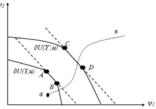
+such that, by Lemma 5, U (Y; u) U (Y0; u) (resp U (Y0; u) U (Y; u)), the set (Y0; u; !) dominates (resp. is domi-nated by) (Y; u; !) in the following sense: for any element 2 (Y; u; !), there exists 0 2 (Y0; u; !) such that 0 (resp. 0 ). See Figure 2. Thus, the fact that S breaks ties along a non-decreasing path yields the desired result, regardless of whether this path passes through (Y; u; !) or
(Y0; u; !).
For necessity, let S be a generalized utilitarian bargaining solution and let u 2 Un be a utility pro…le which does not satisfy Almost TU. Consider a pro-duction possibility set, Y1 RL+, and let y 2 @Y1 be an e¢ cient product mix, so that a 2 EX (y; u) in the economy (Y1; u). By e¢ ciency:
@ui(ai) @xli @ui(ai) @xmi = @uj(aj) @xlj @uj(aj) @xmj = @F1(y) @yl @F1(y) @ym (5)
for any pair of agents i and j and any pair of goods l and m. 8
By continuity, and because the pro…le u does not satisfy Almost TU, there exists an interior exchange e¢ cient distribution b 2 EX (y; u) such that (y; b) is not Pareto e¢ cient in the economy (Y1; u). Therefore,
@ui(bi) @xli @ui(bi) @xmi = @uj (bj ) @xlj @uj (bj ) @xmj for
all i; j 2 N and all l; m 2 L but
@ui(bi) @xli @ui(bi) @xmi = @uj (bj ) @xlj @uj (bj ) @xmj 6= @F1(y) @yl @F1(y) @ym
for some pair l; m of goods. Without loss of generality, suppose that
@ui(bi) @x1i @ui(bi) @x2i = @uj(bj) @x1j @uj(bj) @x2j > @F1(y) @y1 @F1(y) @y2 ; for all i; j 2 N.
Now construct another production possibility set, Y2 RL+, such that y 2 @Y2 and @F2(y) @yl @F2(y) @ym = @ui(bi) @xli @ui(bi) @xmi = @uj (bj ) @xlj @uj (bj ) @xmj
for all l; m 2 L and all i; j 2 N, as shown in Figure 3 in the two-agent case.
8For clarity, we are presenting the proof in the case of all private goods. The proof with
public goods is similar, with the e¢ ciency condition (5) being replaced by the Samuleson condition for these goods (Expression (1)).
Figure 3: Allocation a ( b) is e¢ cient when the production set is Y1 (Y2).
It follows from the construction of Y2 that a is not an e¢ cient allocation in (Y2; u) because @F2(y) @y1 @F2(y) @y2 > @ui(ai) @x1i @ui(ai) @x2i
for all i 2 N. Therefore, there exists an allocation in Y2which Pareto-dominates a. In other words, if we denote by a1 the utility vector corresponding to distribution a, (recall that e¢ ciency of a in the economy (Y1; u) implies that a1 2 @U(Y1; u)) there exists another vector
Figure 4: When utility possibility frontiers cross, solidarity may not hold
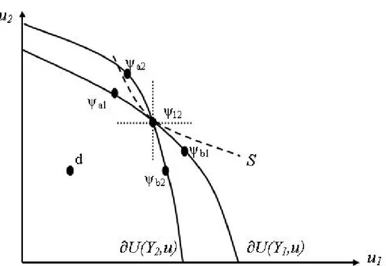
Similarly, because the allocation (y; b) 2 P (Y2; u)nP (Y1; u), there exists a utility vector b12 @U(Y1; u) which dominates b2 2 @U(Y2; u); i.e. b1> b2. From the two previous arguments, and from the continuity of @U (Y1; u) and @U (Y2; u), it must be that @U (Y1; u) and @U (Y2; u) cross at some point in the utility space. Denote by 122 @U(Y1; u) \ @U(Y2; u) such a point.
We now show that there exist bargaining situations where a change from the production possibility set Y1to Y2will bene…t some agents while hurting others. Consider a disagreement point, d 2 U(Y1; u), such that S(U (Y1; u); d) = 12; i.e., such that 12 = arg max 2U(Y1;u)Pi i( i di). Such a disagreement point exists due to the continuity and the strict monotonicity and concavity properties of the i’s, if S 2 G or, if S 2 W, due to the fact that S. breaks ties along a path. Therefore, invoking again the strict monotonicity and concavity of the i’s, and the fact that @U (Y1; u) and @U (Y2; u) cross at 12, it follows that S(U (Y2; u); d) 6= 12.9 Finally, it follows from the fact that U (Y2; u) is convex and comprehensive that S(U (Y2; u); d) neither dominates nor is dominated by S(U (Y1; u); d).
9Recall that we de…ned the disagreement point to be entirely determined by the utility
pro…le and the agents’stand-alone utilities. According to this interpretation, the disagreement point is una¤ected by changes in the joint production possibilities.
Remark 4 Many GUBS do not belong to G [ W; where the 0is are not strictly concave everywhere, for which the proof of Theorem 1 readily applies.
Remark 5 Note that Chun and Thomson (1988)’s one-good economy is a spe-cial case of our economy; with L = 1; and y1 given, it follows that Pi2Nvi = P
x1i and (y1; f (u)) = y1:
Remark 6 In the case of identical utility functions and a symmetric GUBS, if d is on the 45 degree line, the solidarity property is satis…ed even if the bargain-ing solution is not well-behaved. By symmetry of U ( ; u) it is impossible that U (Y1; u) and U (Y2; u) cross at the 45 degree line, yet a symmetric GUBS will always select where @U ( ; u) crosses the 45 degree line.
6
Applications
Theorem 1 has important policy implications. For example, research on fam-ily economics frequently uses bargaining rules – most often the Nash bargain-ing solution – to analyze intrafamily distribution. In this literature parame-ters that change the disagreement point without changing the utility possibility set (McElroy (1990) refers to them as extrahousehold environmental parame-ters) have received substantial attention (Lundberg et al., 1997, Rubalcava and Thomas, 2000, Chiappori et al., 2002), but policies that have the potential to a¤ect the disagreement point as well as the utility possibility set are more dif-…cult to analyze. Examples of policies a¤ecting the utility possibility set and maybe the disagreement point are parental leave policies, policies subsidizing child care, and family taxation. We focus on the latter in the application below.
6.1
Change in Family Tax Policy
Many tax expenditures and provisions in income taxation have a quite complex impact on a family’s full budget set. For example the question of joint or individual taxation changes the household’s production function of income. To …x ideas consider the following model based on Gugl (2009).
Consider a household consisting of two spouses (i = f; m) as the set of agents. Each spouse cares about his or her consumption of a private good (x1i) and consumption of a household public good (x2). Hence, a spouse’s utility function is given by ui(x1i; x2) : Total time endowment of each spouse is denoted by T; which can be divided between employment (li) towards purchasing the private good (x1f+ x1m= y1) and home production (ti) to produce y2.10 Then a spouse’s time constraint is given by li+ ti= T:
Household production is given by
x2= y2(lf; lm) = hf(T lf) + hm(T lm) : (6)
1 0Home production can be interpreted as raising children, but can also stand for taking care
where hf and hmboth satisfy the following properties: hi(0) = 0;@h@tii > 0; and @2h
i
@t2 i 0:
Household Net Income A person’s taxable income is given by the product of his or her wage rate (wi) times the hours worked (li) : Let ind(wili) be the net wage of a person if taxed individually. Given a progressive tax on wages, ind(:) is a strictly increasing and concave function. Thus @@wind
iliwiis the
marginal net-wage rate of spouse i:11
Under joint taxation the net wage of the family as a whole is given by joint
(wflf+ wmlm) : Given a progressive tax on wages, joint(:) is a strictly concave function of the household’s wage,Pi=f;mwili. Then @
joint
@(Pi=f;mwili)wi
is the marginal net-wage rate of spouse i under joint taxation:12
Normalizing the price of the private good to 1, the household budget con-straint is given by
x1f+ x1m= y1= ind(wflf) + ind(wmlm) (7)
under individual taxation, and by
x1f+ x1m= y1= joint(wflf+ wmlm) (8)
under joint taxation.
The couple’s production possibility frontier, @Y; is found by
max (y1; y2)
subject to constraints (6) and (7) under individual taxation and (6) and (8) under joint taxation. A change from individual to joint taxation is a rather complex change and it is possible that @Yindand @Yjoint intersect.13
Let the disagreement point be determined by the stand-alone utility of each spouse, i.e. a person’s utility before marriage. Thus the tax schedule applied in the disagreement point is individual taxation and does not change with a change in family taxation.14 Pollak (2006) argues that even if the disagreement point is determined by a non-cooperative game of spouses and not by the stand-alone utility, it should not change with a change in family taxation. He also concludes that "joint taxation provides incentives for specialization but [...] the
1 1Since the tax schedule starts at a zero tax rate and then increases the tax rate with wage
income, 0 <@@wind
ili 1for any wili> 0and
@ ind(0) @wili = 1:
1 2Again, the tax schedule starts at a zero tax rate and then increases the tax rate with wage
income, so that 0 < @ joint
@ Pi=f;mwili
1for any wili> 0and @
joint(0)
@Pi=f;mwili = 1:
1 3For example, in the US di¤erent tax schedules exist for singles and couples and a couple’s
tax liability is typically more than twice the amount of the tax liability of a single person earning half as much as the family as a whole. This form of joint taxation can lead to Yjoint to be neither a subset of, nor contain, Yind.
distributional e¤ects of joint taxation, which operate through the feasible set, are indeterminant" (Pollak 2006, p. 29). Assuming ATU o¤ers a less ambiguous answer.
Proposition 1 If spouses have utility functions that lead to Almost TU and use a well-behaved GUBS to determine intrafamily distribution, both people either bene…t or lose jointly with a change from individual taxation to joint taxation.
The result presented here establishes conditions under which a change in family taxation is guaranteed to change each family member’s welfare in the same direction provided the disagreement point remains the same. Even if the disagreement point changes, as this would be the case if the tax schedule for singles also changes as part of a fundamental tax reform, Almost TU allows us to decompose the impact of a change in income taxation into a "utility possibility set" e¤ect (family members share the gain or the pain) and a "disagreement point" e¤ect (di¤erent family members may experience changes in their utility at the disagreement point in opposing directions).15
If utility is not Almost TU, it is not clear whether a change in the produc-tion possibility set caused by a change in government policy such as a change from individual taxation to joint taxation will bene…t both spouses in the same direction when a GUBS is used to determine intrafamily distribution, even if the disagreement point is una¤ected by the change in family taxation. In order to evaluate changes in family taxation, it is therefore useful to know whether GUBS plus Almost TU is a good approximation to household behavior.
Almost TU implies that a product mix is e¢ cient independently of distri-bution. Yet empirical studies have found that a change in the disagreement point without changing the utility possibility set of spouses leads to a di¤erent household expenditure pattern or division of labor (e.g. Lundberg et. al, 1997, Rubaclava and Thomas, 2000, Chiappori et al., 2002). A change in expendi-tures on male vs. female clothing or male vs. female entertainment goods when interpreted as changes in expenditures on private consumption goods would be consistent with a model in which spouses have utilities over a household public good (corresponding to y2 above) and disposable income (corresponding to y1 above) that lead to Almost TU. A change in the division of labor, however, either refutes the assumption of Almost TU in the family bargaining context or suggests that more is going on than what is captured in a one period model.16
6.2
Incentive Compatibility
So far, we have considered exogenous changes in the production possibility set and assumed that agents produce e¢ ciently the goods that they share according
1 5Gugl (2009) builds on that result in a two-period bargaining model. The model uses TU
rather than Almost TU.
1 6See e.g. Gugl (2009) for a two-period model with TU that would imply a change in the
to a GUBS. Now suppose that agents choose their actions non-cooperatively to produce goods. In particular, denote by Ai the action set of an agent and by ai 2 Ai a speci…c action taken by agent i: Denote by a i the actions taken by all the other agents except agent i: Each vector a = (ai;a 1) 2 Ai
Y j6=i
Aj
generates y (a) 2 Y Qi2NAi .
Theorem (Incentive Compatibility) If agents use a S 2 G [ W to deter-mine the distribution of a given product mix y (a), the unique subgame perfect Nash equilibrium (SPNE) outcome of the game in which agents sequentially choose their actions is e¢ cient if and only if Almost TU holds. Proof: Su¢ ciency: By Almost TU and Theorem 1. S satis…es solidarity. Therefore, all agents seek to maximize (y(a); u). The fact that agents play a sequential game eliminates the possibility of a coordination problem and, hence, agents will non-cooperatively reach a vector of actions a 2 arg maxa2Qi2NAi
(y(a); u): Necessity follows from Theorem 1: Only if Almost TU holds does a solu-tion in G [ W guarantee that agents have a common goal (i.e., to maximize
(y(a); u)).
6.2.1 Incentive Compatibility and Household Decision Making The above model of spousal decision making also satis…es incentive compatibility in case of Almost TU: Both spouses have an incentive to provide the e¢ cient amount of labor.
Corollary 1 Suppose spouses agree to divide produced goods based on a GUBS but choose their labor supply individually. Each spouse chooses the e¢ cient labor supply if and only if Almost TU holds.
6.2.2 The Rotten Kid Theorem
Theorem 2 has also implications for Gary Becker (1974)’s Rotten Kid Theorem. Bergstrom (1989) formalizes the game that rotten kids play with their altruistic parent: In comparison with the model of spousal decision making introduced above, children now take the place of the spouses; each child’s action impacts the production possibility set of the family. The parent in this game has a …xed amount of money at her disposal and, after observing her kids’actions, deter-mines monetary transfers to its o¤spring by maximizing her altruistic utility function. Thus, the parent’s altruistic preferences play the same role that the GUBS plays in the model of spousal decision making. Therefore, children thus take into account how the parent will react to their actions when they choose their own actions. The Rotten Kid Theorem states that even if the children are completely sel…sh and care only about their own consumption, they will behave as if they are maximizing the parent’s altruistic utility function.
Bergstrom (1989)’s proof of the Rotten Kid Theorem requires TU, because he assumes that the parent treats every child’s utility as a normal good in her
altruistic utility function: Only if any action by a child, given the actions of all the other children results in a restricted utility possibility set in the form of a simplex are all the children guaranteed to bene…t from taking e¢ cient actions. In comparison to Bergstrom, we can weaken the requirement of TU to Almost TU by imposing a stronger, yet reasonable condition on the parent’s altruistic utility function.
Corollary 2 Suppose the parent’s altruistic utility function takes on the form of a general utilitarian social welfare function. Each child behaves as if he/she would maximize the altruistic utility function of the parent if and only if chil-dren’s utility functions lead to Almost TU.
7
Conclusion
Many normatively appealing properties are also crucial in determining posi-tive questions.17 The solidarity property is no exception. We showed that for well-behaved General Utilatarian Bargaining Solutions the solidarity property is satis…ed if and only if Almost TU holds. We then showed that if the agents can agree on how to distribute goods once they are produced, but choose their actions individually, incentive compatibility is satis…ed if and only if the GUBS satis…es the solidarity property.
However, Almost TU is an important subdomain of all utility pro…les and we believe Almost TU, combined with GUBS, to be a useful approach to modelling joint decisions in a variety of economic situations. We are also aware that one may take the opposite view, seeing our result as a damnation of GUBS because Almost TU seems to be rarely satis…ed in practice. In that case the question becomes which class of bargaining solutions should take its place. The one that comes to mind immediately is the egalitarian solution (i.e., the solution that equally splits utility gains) or any other solution that plots a monotonic path through the disagreement point and pays no attention to the shape of the utility possibility set. It is obvious that such solutions satisfy the solidarity property and therefore incentive compatibility regardless of whether the utility pro…le leads to Almost TU or not.
However, such speci…cations are not without their own drawbacks. For ex-ample, consider a two stage game, in which agents can choose actions in the …rst stage that impact their disagreement utility as well as their joint production pos-sibilities in the second stage. The second stage consists of the joint production and distribution of goods as modelled in this paper. The more bargaining solu-tions emphasize the disagreement point the more will agents ine¢ ciently invest in their disagreement utility (Anbarci et al., 2002).
1 7See Moulin (1988) for a link between strong monotonicity in voting rules and strategy
8
References
Anbarci, N, S. Skaperdas and C. Syropoulos, 2002, Comparing Bargaining So-lutions in the Shadow of Con‡ict: How Norms against Threats Can Have Real E¤ects, Journal of Economic Theory 106, 1-16.
Baland, J-M and J. A. Robinson, 2000, Is Child Labor E¢ cient? Journal of Political Economy 108, 663-79.
Becker, Gary S., 1974, A Theory of Social Interactions, Journal of Political Economy 82, 1063-94.
Bergstrom, Th. C., 1989, A Fresh Look at the Rotten Kid Theorem – and Other Household Mysteries, Journal of Political Economy 97, 1138-59.
Bergstrom, Th. C. and R. C. Cornes, 1983, Independence of Allocative E¢ ciency from Distribution in the Theory of Public Goods, Econometrica 51, 1753-66.
Bergstrom, Th. C. and R. C. Cornes, 1981, Gorman and Musgrave are Dual: An Antipodean Theorem on Public Goods, Economic Letters 7, 371-378.
Bergstrom, Th. C. and H. R. Varian, 1985, When do market games have transferable utility? Journal of Economic Theory 35, 222-33.
Bommier, A. and P. Dubois, 2004, Rotten Parents and Child Labor, Journal of Political Economy 112, 240-248.
Chiappori, Pierre-André, Bernard Fortin, and Guy Lacroix, 2002; Marriage Market, Divorce Legislation, and Household Labor Supply, Journal of Political Economy 110, 37-72.
Chun, Y. and W. Thomson, 1988, Monotonicity Properties of Bargaining Solutions When Applied to Economics” Mathematical Social Sciences 15, 11-27.
Gugl, Elisabeth, 2009, Income splitting, specialization, and intra-family dis-tribution, Canadian Journal of Economics 42, 1050-71.
Kalai, E. and M. Smorodinsky, 1975, Other Solutions to Nash’s Bargaining Problem, Econometrica 43, 513-18.
Lundberg, Shelly J., Robert A. Pollak and Terence J. Wales, 1997, Do Hus-bands and Wives Pool Their Resources? Evidence from the United Kingdom Child Bene…t, Journal of Human Resources 32, 463-480.
Mas-Colell, A., M. D. Whinston and J. R. Green, 1995, Microeconomic Theory (Oxford University Press, New York).
Moulin, H., 1988, Axioms of Cooperative Decision Making (Cambridge Uni-versity Press, Cambridge).
Nash, J. F. Jr., 1950, The Bargaining Problem, Econometrica 18, 155-62. Pollak, R. A., 2006; Family Bargaining and Taxes: A Prolegomenon to the Analysis of Joint Taxation, Forthcoming in CESifo Economic Studies + MIT Press book
Rubalcava, Luis and Duncan Thomas, 2000, Family Bargaining and Welfare, Working Paper CCPR-007-00, California Center of Population Research.
Rubinstein, A., Z. Safra, and W. Thomson, 1992, On the Interpretation of the Nash Bargaining Solution and Its Extensions to Non-Expected Utility Preferences, Econometrica 60, 1171-81.
Sprumont, Y., 2008, Monotonicity and Solidarity Axioms in Economics and Game Theory, in Rational Choice and Social Welfare, Springer Berlin Heidelberg Eds. 71-94.
Xu, Y. and N. Yoshihara, 2008, The Behaviour of Solutions to Bargaining Problems on the Basis of Solidarity, Japanese Economic Review 59,133-138.
9
Appendix
9.1
Proof of Example 3
To …nd (y; x) 2 P (Y; u) ; …rst note that any e¢ cient allocation must satisfy the
following: 8 < : y1= x11+ x12 y2= x21 y3= x32 To …nd P (Y; u) and @U (Y; u) we solve:
max x11;x12;x21;x32
u (x11; x21) s.t. 2= u (x12; x32)
x11+ x12+ p2x21+ p3x32= I This problem is equivalent to simultaneously
max x11;x12 u (x11; x21) s.t. x11+ x12+ p2x21= I1 and max x21;x32 u (x12; x32) s.t. x11+ p3x32= I2 subject to I1+ I2= I:
It is obvious that the higher agent 1’s share of I; the higher her utility. Thus each 2 @U (Y; u) must be associated with a di¤erent distribution of I where agent 1 gains utility with every increase in her share and agent 2 loses utility with every decrease in his share. Homogeneity of degree one implies homotheticity which in turn implies that it is optimal for agent 1 to consume (x11; x21) in the same proportion as before as her share of I increases. The same is true for agent 2 with respect to (x12; x32) : By homogeneity of degree 1 of the utility functions, we also know that an increase in the share of I causes a proportional increase in ui: Hence, the indirect utility function of agent 1 writes as follows
where
e (p2) = max x11;x21
u (x11; x21) s.t. x11+ p2x21= 1
and we can write the indirect utility function of agent 2 as (p3; I2) =e (p3) I2 where e (p3) = max x12;x32 u (x12; x32) s.t. x12+ p3x32= 1
Di¤erentiating with respect to Ii: @ i @Ii
=e (pi+1) :
This implies that as agent 1’s share of I increases by one unit, her utility in-creases bye (p2), and agent 2’s utility decreases bye (p3) : Independent of how many units of I are already allocated to person 1, the decrease in person 2’s utility and the increase in person 1’s utility will always be the same as person 1 receives an additional unit of I: Therefore any ( 1; 2) is found by
2= (Y; u2) e (p3 ) e (p2) 1
:
Also note that
e (p3) e (p2) =e (p3) I e (p2) I = (Y; u2) (Y; u1) : Thus @U (Y; u) = 2 R2+j 1 (Y; u1) + 2 (Y; u2) = 1 :
Only in the special case in which p2= p3= p such that Y = y 2 R3+jy1+ p (y2+ y3) = I we have
(Y; u1) =e (p) I = (Y; u2) : Then