2007 — Construction of nacelle power-curve following Markov's theory

ECOLE DE TECHNOLOGIE SUPERIEURE UNFVERSITE DU QUEBEC

THESIS PRESENTED TO

ECOLE DE TECHNOLOGIE SUPERIEURE

IN PARTIAL FULFILLMENT OF THE REQUIREMENTS FOR THE DEGREE OF MASTER OF MECHANICAL ENGINEERING

M. Eng.

BY

POULIN, Jonathan

CONSTRUCTION OF NACELLE POWER-CURVE FOLLOWING MARKOV'S THEORY

MONTREAL, OCTOBER 29 2007 ) Copyright 2007 reserved by Jonathan Poulin

Mr. Christian Masson, Thesis Supervisor

Departement de genie mecanique a I'Ecole de technologic superieure

Ms. Saskia Honhoff, Thesis Co-supervisor General Electric, Wind Energy

M. Jean-Pierre Kenne, President of the Board of Examiners

Departement de genie mecanique a I'Ecole de technologic superieure

M. Simon Joncas, Examiner

Departement de genie de la production automatisee a I'Ecole de technologic superieure

THIS THESIS HAS BEEN PRESENTED AND DEFENDED BEFORE A BOARD OF EXAMINERS

SEPTEMBER 28, 2007

ACKNOWLEDGMENT

First, I would like to thank my thesis supervisor Christian Masson, for giving me the opportunity to make my master's thesis in wind-turbine technology. Your support, knowledge and availability was well appreciated. You give me much more than simply answer my questions! Thank you for everything.

I also would like to thanks my thesis co-supervisor Saskia Honhoff, from General Electric, in Germany. Thank you for your hospitality, when I went 3 weeks in Germany. Also thank you for all the time you spent with me in order to realise this thesis.

Thank you to all my friends and family, especially my father Luc, my mother Carole and her husband Michel. This thesis wouldn't have been possible without you. You made me believe that it was possible to make this project and did support me on the toughest moments. I'm gratefiil to have you for parents... Thank you! Merci!

Special thanks to my girlfriend Marie-Josee, thank you for loving me, being with me all that time and helping me in the realisation of this thesis. The past one and half year with you was exceptional... Merci Bibi!

POULIN, Jonathan ABSTRACT

The standard procedure to constmct a power curve is the lEC standard. However, this model contains some flaws. In fact, by averaging the power inside a bin speed the power obtained isn't precise, since the power is directly affected by the turbulence intensity of the wind speed. Moreover, it requires long time to evaluate the influence of different settings with this method. The solution proposed in this thesis is to implement a novel method to construct a power curve, which is by following the Markov's theory. This method calculates the stationary power with a stochastic approach, which is more precise and should take less time than the standard procedure. Nonetheless, the construction of a power curve with the meteorological-mast (MM) anemometer isn't always feasible. In addition, the distance between the MM and the turbine can reduce the correlation of the wind speed read at the MM anemometer and the one which hit the blades of the turbine. Thus, to correct that, the construction of the power curve should be implemented on the nacelle anemometer.

The final objective of this master thesis is to implement a Markov power-curve program, which will calculate the stationary power with the nacelle anemometer at each speed bin. Furthermore, this thesis will evaluate and optimise the parameters to obtain the best power curve following this novel method. Finally, the evaluation of the measurement time required to construct this type of power curve will be executed.

Albeit the power curves obtained following this new method aren't stable, this thesis proposes the median to calculate the conditional moment, since the results are less affected by the turbulence intensity. Besides, it also proposes to average the wind speed over a period of two minutes, when using the nacelle anemometer, to eliminate the fast fluctuations of the wind speed due to the blade passage. Moreover, the utilisation of the data averaged over different periods of time doesn't change the result of the power curve. However, the time required to construct a Markov power-curve isn't affected by the averaging time of the data. Nevertheless, this novel method is a little bit faster than the lEC procedure.

Further improvement should be done in the power-curve program. The software amelioration should make the resuUs more stable and more accurate. In addition, the required time to construct a Markov power-curve might decrease again. The first recommendation is to verify with more data sets the rotor-position filter effect, when using the nacelle anemometer to construct a Markov power-curve. The second recommendation could be to correct the second minimum problem when calculating the stationary power with the minimal potential. A method to correct that will be to optimize the relaxation-time interval to determine the drift.

CONSTRUCTION O F NACELLE POWER-CURV E FOLLOWIN G MARKOV'S THEOR Y

POULIN, Jonathan

RESUME

La procedure standard pour construire une courbe de puissance est la norme lEC. Toutefois, ce modele contient quelques faiblesses. Une de ses faiblesses est le fait de moyenner les puissances, ce qui engendre des erreurs puisque les puissances obtenues, sur la courbe de puissance, sont grandement influencees par I'intensite de turbulence de la vitesse du vent. De plus, cette norme pent demander beaucoup de temps pour evaluer 1'influence de divers parametres sur une eolienne. La solution proposee dans ce memoire est d'implementer une nouvelle methode, en suivant la theorie de Markov, pour calculer les courbes de puissance. Cette methode calcule la puissance stationnaire avec une approche stochastique, laquelle est plus precise et s'effectue en un plus court laps de temps. II arrive aussi que le calcul d'une courbe de puissance puisse etre impossible a effectuer avec I'anemometre a la tour meteorologique, il faut done creer une fonction de transfert pour I'implementer a I'anemometre a la nacelle de I'eolienne.

L'objectif final de ce memoire est de creer un programme qui va constmire une courbe de puissance, avec I'anemometre a la nacelle, en suivant la theorie de Markov, tout en evaluant et opfimisant I'influence de divers parametres. Finalement, un autre objectif est I'analyse du temps minimum requis avec ce nouveau modele pour constmire une courbe de puissance. Bien que les resultats obtenus ne soient pas stables, ni parfait, ce memoire propose la mediane pour calculer le moment conditionnel, puisque les resultats sont moins affectes par I'intensite de turbulence. Par la suite, il propose aussi de moyenner les vitesses du vent sur une periode de deux minutes, lorsque la vitesse du vent est lue sur I'anemometre a la nacelle, afin d'eliminer les fluctuations rapide du vent causees par le passage des pales de I'eolierme. Cependant, le temps necessaire a la construction d'une courbe de puissance en suivant la theorie de Markov n'est pas affectee par les donnees moyennces a differents intervalles de temps. Par contre, cette nouvelle methode pent constmire une courbe de puissance en un temps plus rapide que la norme lEC.

De plus amples ameliorations doivent etre effectue dans le programme qui constmit la courbe de puissance avec Markov. En fait, I'amelioration du programme permettrait d'obtenir des resultats plus stables, et done plus precis. Par le fait meme, cette amelioration pourrait faire en sorte d'effectuer une courbe de puissance en un temps plus court. La premiere recommandation est de verifier I'impact du filtrage pour la posifion du rotor, avec un plus grand nombre d'eoliennes. La deuxieme recommandation est de corriger I'apparition du deuxieme minimum. Une methode pour le corriger est d'optimiser I'intervalle du temps de relaxation.

INTRODUCTION 1 CHAPTER 1 LITERATURE REVIEW 5

1.1 Intemafional Electrotechnical Commission (lEC) standard 5

1.1.1 Performance test on a wind turbine 6 1.2 lEC flaws 11

1.3 Markov process 12 1.4 GE's works 12 1.5 University of Oldenburg's contribution 15

1.5.1 Simulated-data and power-curve programs 15 1.5.2 Articles made by the University of Oldenburg 16

CHAPTER 2 MATHEMATICAL MODEL 18 2.1 Langevin equation for Brownian motion 18

2.2 Fokker-Planck equation 21 2.3 Stochastic processes 22 2.4 Markov property 23 2.5 Coefficients esfimafion 23 CHAPTER 3 WIND-TURBINES DESCRIPTION 27

3.1 Klondike-ll 27 3.2 Wietmarschen 29

3.3 Prettin 31 CHAPTER 4 POWER CURVE CONSTRUCTED WITH THE

METEOROLOGICAL-MAST ANEMOMETER 34

4.1 Default power-curve 36 4.2 Power-states range filter 40

4.3 Method to calculate the conditional moment 42

4.3.1 Median 43 4.3.2 Most frequent power-difference 45

4.3.3 Power-differences filter 48

4.4 Method to calculate the stationary power curve 50

4.5 Method to calculate the drift 52

4.6 Power-states number 54 4.7 Averaging time 56 4.8 Wind speed averaging 58 4.9 Synthesis of all parameters 61 CHAPTER 5 POWER CURVE CONSTRUCTED WITH THE NACELLE

ANEMOMETER 63 5.1 Wind-speed averaging at the nacelle anemometer 64

VII

5.2 Rotor-position filter 66 5.3 Averaging time below 1 second 67

CHAPTER 6 VALIDATION OF THE POWER CURVE WITH WIETMARSCHEN

AND PRETTIN TURBINES 70 6.1 Meteorological-mast anemometer 70

6.2 Nacelle anemometer 75 CHAPTER 7 TIME REQUIRED TO CONSTRUCT A NACELLE POWER-CURVE

FOLLOWING MARKOV'S THEORY 81

CONCLUSION 84 RECOMMENDATIONS 87

APPENDIX I FLOW CHART: SOFTWARE TO CONSTRUCT THE STATIONARY

POWER CURVE 89 APPENDIX 11 POWER ERROR FOR THE DATA AVERAGED AT 1 SECOND 95

APPENDIX III POWER ERROR FOR THE DATA AVERAGED AT 0,1 SECOND 98 APPENDIX IV CONDITIONAL MOMENT IN FUNCTION OF THE RELAXATION

TIME 101 BIBLIOGRAPHY 105

Figure 1.1 Requirements as to distance of the meteorological mast and maximum

allowed measurement sectors [9] 7 Figure 1.2 Sectors to exclude due to wakes of neighbouring and operating wind turbines

and significant obstacles [9] 8 Figure 1.3 GE's simulated data created around a theoretical power-curve [13] 14

Figure 1.4 Power curve obtained by the University of Oldenburg with their

simulated-data and power-curve programs [6] 16 Figure 1.5 Power curves obtained for a simulated data set [7] 17

Figure 2.1 Example of conditional moment in function of the relaxation time (i) 25 Figure 2.2 Comparison of the minimal potential with the zero crossing to determine the

stationary power output [13] 26 Figure 3.1 Klondike-II site located in U.S.A. in the Oregon State 28

Figure 3.2 Scatter plot of the power in fianction of the MM wind speed at an averaged

time of 1 second for Klondike-10 29 Figure 3.3 Wietmarschen site located in Germany 30 Figure 3.4 Scatter plot of the power in function of the MM wind speed at an averaged

time of 1 second for Wietmarschen-1 31 Figure 3.5 Prettin site located in Germany 32 Figure 3.6 Scatter plot of the power in fiinction of the MM wind speed at an averaged

time of 1 second for Prettin-5 33 Figure 4.1 Scatter plot of the simulated data around the theoretical power-curve [6] 35

Figure 4.2 Defauh power-curve for the simulated data 37 Figure 4.3 Default power-curve for the MM anemometer of Klondike-10 37

Figure 4.4 Linear-regression method to determine the power at the bin speed of 6,25 m/s

IX

Figure 4.5 Minimal-potential method to determine the power at the bin speed of 6,25 m/s

for Klondike-10 39 Figure 4.6 Conditional moment in fiinction of the relaxation fime at the bin speed of 6,25

m/s at the power state of 579 kW for Klondike-10 40 Figure 4.7 Comparison of different power-states range filter for the simulated data 42

Figure 4.8 Comparison of different power-states range filter for the MM anemometer of

Klondike-10 42 Figure 4.9 Histogram of the power difference for the bin speed of 9,25 m/s, for the

power state of 1450 kW and for the relaxation time (T) of 5 seconds for

Klondike-10 43 Figure 4.10 Comparison of the mean with the median to calculate the power curve for the

simulated data 44 Figure 4.11 Comparison of the mean with the median to calculate the power curve for the

MM anemometer of Klondike-10 45 Figure 4.12 Example of distribution for the power difference 46

Figure 4.13 Example of distribution for the power difference at 50% of the highest

number of data 47 Figure 4.14 Comparison of the median with the most frequent to calculate the power

curve for the MM anemometer of Klondike-10 48 Figure 4.15 Comparison of the median with the power-differences filter to calculate the

power curve for the simulated data 49 Figure 4.16 Comparison of the median with the power-differences filter to calculate the

power curve for the MM anemometer of Klondike-10 49 Figure 4.17 Comparison of the median with the power-differences filter to calculate the

power curve for the MM anemometer of Wietmarschen-2 50 Figure 4.18 Comparison of the minimal potenfial with the linear regression to calculate

the power curve for the simulated data 52 Figure 4.19 Comparison of the minimal potential with the linear regression to calculate

the power curve for the MM anemometer of Klondike-10 52 Figure 4.20 Comparison of the power curve with different methods to calculate the drift

Figure 4.21 Comparison of the power curve with different methods to calculate the drift

for the MM anemometer of Klondike-10 54 Figure 4.22 Comparison of different number of power states to calculate the power curve

for the simulated data 55 Figure 4.23 Comparison of different number of power states to calculate the power curve

for the MM anemometer of Klondike-10 56 Figure 4.24 Comparison between the averaging times higher than 1 second to constmct

the power curve for the MM anemometer of Klondike-10 57 Figure 4.25 Comparison between the averaging times shorter than 1 second to construct

the power curve for the MM anemometer of Klondike-10 58 Figure 4.26 Comparison of different averaging times of the wind speed to constmct the

power curve for the simulated data 60 Figure 4.27 Comparison of different averaging times of the wind speed to constmct the

power curve for the MM anemometer of Klondike-10 60 Figure 4.28 Comparison of different averaging times of the wind speed to constmct the

power curve for the MM anemometer of Wietmarschen-2 61 Figure 5.1 Correlation between the MM and the nacelle anemometer for Klondike-10 63

Figure 5.2 Default power-curve constmcted for the nacelle anemometer of Klondike-10 64 Figure 5.3 Comparison of different wind-speed averaging time for the power curve

constmcted for the nacelle anemometer of Klondike-10 66 Figure 5.4 Comparison of the rotor-position filter for the power curve constmcted for the

nacelle anemometer of Klondike-10 67 Figure 5.5 Comparison of the time averaging for the power curve constmcted for the

nacelle anemometer of Klondike-10 68 Figure 6.1 Power curve obtained with the default parameters for the MM anemometer of

Prettin-4 71 Figure 6.2 Power curve obtained with the default parameters for the MM anemometer of

Prettin-5 72 Figure 6.3 Power curve obtained with the default parameters for the MM anemometer of

XI

Figure 6.4 Power curve obtained with the default parameters for the MM anemometer of

Wietmarschen-2 73 Figure 6.5 Comparison of the time averaging for the power curve constmcted for the

MM anemometer of Wietmarschen-1 74 Figure 6.6 Comparison of the time averaging for the power curve constmcted for the

MM anemometer of Wietmarschen-2 75 Figure 6.7 Power curve obtained with the default parameters for the nacelle anemometer

of Prettin-4 76 Figure 6.8 Power curve obtained with the default parameters for the nacelle anemometer

of Prettin-5 77 Figure 6.9 Power curve obtained with the default parameters for the nacelle anemometer

of Wietmarschen-1 77 Figure 6.10 Power curve obtained with the default parameters for the nacelle anemometer

of Wietmarschen-2 78 Figure 6.11 Comparison of the time averaging for the power curve constmcted for the

nacelle anemometer of Wietmarschen-1 79 Figure 6.12 Comparison of the time averaging for the power curve constmcted for the

nacelle anemometer of Wietmarschen-2 79 Figure 7.1 Power error at each bin speed in fiinction of the time for the data averaged at

1 second 82 Figure 7.2 Power error at each bin speed in fianction of the time for the data averaged at

A Swept area of the wind-turbine rotor [m^] AEP Annual Energy Production [MWh]

5iomin Measured air pressure averaged over 10 minutes [N/m ] Cp C • d D D<'> r)(I) noise-ind De F F(V) Fc Ff

k

L

Power coefficient in bin z

Distance between the rotor and the anemometer [m] Rotor diameter [m]

Drift coefficient Noise-induced drift

Equivalent rotor diameter [m] Force [N]

Rayleigh cumulative probability distribution function for wind speed Damping force [N]

Flucmation force [N] Height of obstacle [m] Width of obstacle [m] Boltzmann's constant [J/ °K]

Distance between the obstacle and the MM [m] Mass [kg]

Conditional moment N Number of bins

XIll

Ni Number of 10 minutes data sets in bin / Nh Number of hours in one year [8760 hours] p Fluctuation around the stafionary power [W] P Power output [W]

Pfix Stationary power [W]

Pi Normalized an averaged power output in bin / [W] P„ Simulated power output [W]

P„,ij Normalized power output of data sety in bin / [W] Psiaie Power state [W]

Psiationary Stationary power [W]

P,h Theoretical power output [W] Q Conditional probability

RQ Gas constant of dry air [287.05 J/(kg x "K)]

/ Time (s)

T Temperature (°K)

T\omm Temperature averaged over 10 minutes [°K]

77 Turbulence intensity

w„ Simulated wind speed

U Horizontal mean wind speed [m/s] V Wind speed [m/s]

f^iomin Measured wind speed averaged over 10 minutes [m/s]

Vave Annual average wind speed at hub height [m/s]

Vi Normalized and averaged wind speed in bin z [m/s] Vn Normalized wind speed [m/s]

V„,ij Normalized wind speed of data sety in bin / [m/s] W Probability-density fianction

a Additional excluded sector [degree] /? Noise influence

y Relaxation parameter

r Fluctuating force per unit mass [N/kg] r„ Gamma function

5 Dirac delta function

£ Attraction from averaged wind speed (^ Stochastic variable

rjGB Gear box ratio r]ioi Total efficiency A Mass flow [kg/s]

V Speed [m/s]

V Acceleration [m/s ] p Air density [kg/m^]

po Reference air density [kg/m^]

Pioniin Derived 10 minutes averaged air density [kg/m^] cr„ Standard deviation of the horizontal wind speed [m/s] X Relaxation time [s]

XV

(p Influenced rotor position [degree] (o Average generator speed [rpm]

In recent years, new demand for cleaner and renewable energy sources has arrived, since the pollution has became a global waming, with his non-desirable effect on the earth, to most of the population. Indeed, coal and oil energy, fuel emissions and others sources of pollution have a negative impact on globe health. The planet has the advantage to produce natural energy, and one of them comes from the wind, which can be found anywhere around the world.

Today, more than 74 GW of wind energy are installed all around the worlds, which represent over 100 000 wind turbines in 70 countries [5]. Furthermore, the low cost of wind energy, which is less expansive than the coal, oil and nuclear, is a favourable element to continue to investigate in this field. In fact, it costs approximately 3,5 to 4 cents per kilowatt hour and declining [3].

Introduction to wind turbine

The production of wind energy is done by the exploitation of a wind turbine. Basically, when wind hits the blades of the turbine, it creates a rotation of the rotor, and this rotation coupled with the torque produce the power. Afterwards, this mechanical power is transformed in electrical power by a generator.

The wind power is a cubic fiinction of the wind speed. However, the turbine isn't working at really low wind speed due to the fact it will cost more electricity that it will produce. Therefore, the mrbine start-up occurs when the wind speed reaches a point, where there is enough energy into it to efficiently use the turbine, which is referred to as the cut-in wind speed. Once the turbine has reached the cut-in wind speed, its power will increase with a cubic relation of the wind speed, until it attains the rated power. The rated power is the power capacity of the turbine. Once it is reached, the power will stay the same, even if the wind speed continues to increase. This is a preventive measure, since the turbine stresses would be

too high if the power would continue to increase. For the same reason, the turbine will stop if the wind speed is too high, which is called the cut-off wind speed.

Objectives an d methodolog y

Today, the wind-energy companies need to follow the lEC procedure to constmct a power curve. A power curve is a curve which expresses the power of the turbine in function of the wind speed. However, this standard procedure (lEC) has some flaws, since it can take some considerable time in order to constmct power curves. Moreover, by utilising an averaging method, like the lEC does, it is not accurate to calculate the power since it is a cubic function of the wind speed. Consequently, the measurements of different settings are long and the results aren't precise.

To avoid the seasonal variation when evaluating different settings and to reduce costs, these problems should be solved. One of the solutions is to evaluate a new method to constmct a power curve. The method analysed in this master thesis is the constmction of a power curve following Markov's theory. This method is a stochastic evaluation of the power curve. However, a problem occurs when using this method because it requires data averaged over a short period, and also because the turbine can be far away from the meteorological mast (MM). Thus, the correlation between the MM anemometer and the power output of the turbine is reduced or lost. Furthermore, the utilisation of the MM anemometer isn't always feasible, because it is too far away of the turbine, or the terrain is highly complex. For all these reasons, the analysis should be implemented on the nacelle anemometer.

This thesis proposes a program which can calculate a power curve with this novel method. In addition, it also recommends a transfer function to correlate the wind speed from the MM anemometer to the nacelle anemometer, with the respect of Markov's theory.

In order to have a better understanding of the thesis, the objectives, the problems and the results; the description of the thesis stmcmre is explained here.

In Chapter 1, a literature review, of what was made before in this field, is done. The standards and the results of the previous research from different contributors are presented. Moreover, the lEC flaws are exposed and proved, and a short introduction of the novel theory is done to acquire basic knowledge.

Then, Chapter 2 will demonstrate the mathematical model of a power curve constmcted with the Markov's theory. Therefore, the equations will be shown and the method to determine different coefficients will be revealed.

Next, Chapter 3 will introduce the wind turbines analysed in this master thesis. Consequently, the location of the wind farms, the operating data and the limitation of the analysis on those turbines are described.

After that. Chapter 4 will analyse the influence of each parameter to constmct a Markov power-curve with the MM anemometer. In fact, an optimisation of each parameter is done to determine the best power curve for all turbines studied.

Chapter 5 will optimise the parameters to constmct the best Markov power-curve, but this time with the nacelle anemometer.

Afterwards, Chapter 6 will only validate the best parameters with other sites or turbines. Therefore, power curves following Markov's theory will be constmcted with optimised parameters of others turbines and data sets, to verify the quality of the power curve for those sites or turbines.

Finally, Chapter 7 will determine the minimal amount of data required to constmct a good power curve with the nacelle anemometer and compare this result with the lEC standard.

LITERATURE REVIE W

The constmction of a power curve for a specific site is well known and well defined. When constmcted, this power curve is used to determine the Annual Energy Production (AEP) of the site. However, the constmction of a power curve requires data collection over a certain period of time like power, wind speed, air density, wind direction, etc. This chapter presents a literature review of the standard procedure to constmct a power curve on wind farms, the flaws of the standard procedure and a new method to constmct a power curve.

LI Internationa l Electrotechnica l Commissio n (lEC ) standar d

The International Electrotechnical Commission ( E C ) is a worldwide organization for standardization comprising all national electrotechnical committees. The objective of lEC is to promote international co-operation on all questions concerning standardization in the electrical and electronic fields [9]. This committee is therefore present in wind-energy technology, where their standards are applied all around the world.

The official method to constmct a power curve is explained in one of the lEC standard. Wind-farm and wind-mrbine companies are recommended to follow this standard, otherwise customers won't have any reference when analysing which companies have the best turbines for their projects.

There are two different lEC standards in the wind-energy industry used to constmct power curves. The first one (lEC 61400-12-1) is a standard utilised when the energy calculated at the turbine is made with the MM anemometer, while the second one (lEC 61400-12-2) is a standard utilised when the energy calculated at the turbine is made with the nacelle anemometer, which is normally positioned on the top of the wind turbine.

1.1.1 Performanc e test on a wind turbine

The performance test is used to verify if the output power giving by the turbine is the same as what was defined in the manufacturer-customer contract. This validation requires a few steps. Firstly, it is required to find a location for the MM. The second step is to determine the measurement sector. Thirdly, the measurements can be done and the wind speed needs to be normalized with respect to air density. Then, the power curve, the AEP and the power coefficient can be calculated.

Meteorological-mast location

When positioning the MM, it should not be installed too close of the wind turbine, because the wind speed will be influenced. However, it should neither be installed too far away from the mrbine, since the correlation between the wind speed and the electrical power output of the wind turbine will be reduced.

The ideal distance to which the meteorological mast can be installed from the turbine is 2,5 times the rotor diameter (D) of the wind turbine. However, it also can be installed at a distance between two and four times the rotor diameter, from the wind mrbine. In fact if the MM is too close of the turbine, then the wind speed read at the MM anemometer might be influenced by the blade passage, while if the MM is too far of the turbine then the correlation between the MM and the turbine could be lost. Most of the times, the best meteorological-mast position will be upwind of the turbine in the direction where the most dominant wind is expected to come during the test [9].

Measurement sector

Due to the MM being in the wake of the wind turbine for certain sectors, it is necessary to exclude those sectors during the test. Indeed, when the wind passes trough a turbine, it affects its speed. Consequently, the wind speed obtained at the MM isn't the real wind speed. Figure

.y / / / / /

1

1 '

N

Mast 1c: vv -11.1 ti.rb ne cei Mast a y ' Win d tjrbi'ie y - i (re line :4D ^x Dis:ar-c e of rretecrolcgy 2i.i} \ nas:to;vln s 2r/snr.l 4r> 7 .^ \ 2.?Di s reccirnended \ \ \ tr"-^.^^ '\ Distuitje d i.ec:or •<4.. due to wcike c* / win d tLirLiine or 1 me:e3'olog y 'na-i / (Anne x A;.: / a t 2I> hV i at2,.5D:74 ' at 4D .59 ' \ 1 i /

\ ^ / Maximu m measuremen: sector:

./ at . 21); HV

t \ / a t 2.5Z': 23iV

/ a t - J : ViV

Y

Figure 1.1 Requirements as to distance of the meteorological mast and maximum allowed measurement sectors [9].

However, those sectors might be insufficient when others turbines or significant obstacles are present on the wind farm. In fact, those obstacles affect the wind speed, so the measurement sector should be reduced. The distance (Le) between the obstacle and the meteorological mast, the equivalent rotor diameter (De) and the size of the obstacle are the dimensions to be taken into account. If the obstacle isn't a wind turbine, then the equivalent rotor diameter should be calculated.

D =.2V . h+K

Afterwards, with the equivalent diameter and the distance, the disturbed sector of the obstacle can be defined.

2 5D

a = 1.3arctan(-—^-l-.15)-l-10 (1.2)

In the equation (1.2), a is the additional sector to be excluded. The additional sector excluded also can be found with the graphic of Figure 1.2.

^;0 SCI 1 « o h -0 \ .'-' 1 1 i 1 1 1 i 1 «= 1,3arc!ari2,5I>e,'I e + 0,15) + 10 0f«= • . 3 „L ... . r \ ^ Urdistu'be d i f DiStU 1 rSed 1 ! 1 1 3r-tarii:2.5A-.'.in ^ 0 . ' oi + 1 0 r j 1 1 ) i 1 8 ' 0 1 2

RcUntivir diolJiice LfiD. o r L ^ ' D ,

13 2 0 2 2

Figure 1.2 Sectors to exclude due to wakes of neighbouring and operating wind

turbines and significant obstacles [9].

Data normalization

In order to execute a performance test following the lEC standard, it is necessary to average all variables measured over ten minutes. Therefore, the air density, the pressure, the wind speed, the power, and other variables are averaged on a period of ten minutes. However, the data collected aren't normalized. In fact, the calculation of the power in function of the wind speed is given by [11]:

temperature [9].

^ ^ -^lOmin (1.4)

•'^O-'lOmin

Because the air density isn't a constant, it is required to normalize the data to the sea level air density (po), which is 1,225 kg/m^ Moreover, GE's wind turbines are with active power-control. In that case, the normalization should be applied to the wind speed, according to the lEC procedure. However, if the turbines are with passive power-control, then the normalization should be applied to the power output [9].

V =V 'n " ^ lOmi n ^Ao ^ mm 1/3 V A J (1.5) Wind-turbine performances

The turbine performances are characterized by the calculation of the power curve, the AEP and the power coefficient. According to the lEC standard, those measures of performance are determined by applying the method of bins. The first step in applying the method of bins consists of calculating the mean value of the power and the wind speed at each 0,5 m/s bins for the normalized data sets [9].

1

10

P-—TP-(1.7)

Then, it is possible to calculate the annual energy production from the wind turbine. In order to do that, a Rayleigh distribution is used as the reference wind speed frequency distribution [9].

AEP = N,Y^'jF(V,)-F(V,^,)]

fP.,+P

F(F) = l-exp V

, V

^2^ _(1.9)

Finally, the power coefficient can be calculated with equation (1.10). At rated power, the power coefficient will drop significandy with the respect to equation (1.10), since the wind speed is increasing while the power stays constant.

C . „ = j

PoAV,'

(1.10)

If we want to utilise the nacelle anemometer to constmct a power curve, the correlation between the nacelle anemometer and the MM anemometer should be done following the lEC 61400-12-2 procedure [12]. This correlafion is done because the wind is affected by the blade passage. This correlation can be executed by following the bins method. In reality, the real speed, from the meteorological-mast anemometer, is in function of the nacelle wind-speed. Therefore, at each bin speed a linear regression is done between those two wind speeds.

1.2 lE C flaws

Even though the only standard method to calculate a power curve is the lEC 61400-12-1 procedure, this method contains some flaws. Indeed, an lEC power curve cannot be constmcted before the data base reaches 180 hours [9]. Therefore, the performance test can be long, since the wind isn't always in the measurement sector and the turbine might not work properly for a certain period of time.

Moreover, averaging the power and the wind speed gives imprecision because it is not a linear function. In fact, the power is a cubic fiinction of the wind speed, as shown in equation (1.3). Consequently, the power curve is obtained from those measurements by ensemble averages denoted as (y{t))-^(^P(V(t))) [1]. The nonlinearity of this power curve is also spoiled by mrbulent winds at the specific turbine site, which is caused by the obstacles, weather, topography etc. The turbulence of the wind is described by the turbulence intensity

(TI).

TI = aJU (1.11) The mrbulent winds aren't considered in the standard procedure and lead to the following

inequality:

p({V(t)))^{P(V(t)))

Therefore, if we focus on the instantaneous electrical wind-turbine power, instead of the ensemble averages we thus obtain [1]:

12

Where Pfix(V) denotes the stationary power output as fiinction of the wind speed and p(t) denotes the respective temporal flucmations around this stationary power output. The performance test is utilised to verify if the turbine gives the power it is suppose to give at a certain wind speed. Consequently, the power of interest is the stationary power, instead of the average power (P(t)), since this power doesn't include or is less influenced by the wind turbulences, pitch-angle changes, shutdown states, or others non-desirable effect, which cause the scatter plot to be greater. A method to obtain numerically the stationary power curve is to utilise Markov's theory, which is described by a generalised one-dimensional Langevin equation. The mathematical model of those equations is demonstrated in the Chapter 2.

1.3 Marko v process

In order to understand the works explained in this chapter, an introduction of Markov process is described here. In fact, GE's and the University of Oldenburg works explain how they have constmcted a power curve following Markov's theory. Therefore, a brief explication of Markov process is required.

The Markov process can be applied in different applications, like the physics, the statistics, the electrics or the bioinformatics. First, a Markov property is a stochastic process, with also the conditional-probability of the distribution of future states of the process, and this conditional-probability depends only of the present state and not on any past states [19]. Thus, the distribution of fijture states depends only of the present state and not how it occurs at the current state. Therefore, the Markov process is a memory-less process [13]. More details on this property will be done later in the Chapter 2, and also the equations of this process will be explained.

1.4 GE' s works

The Wind-Energy division of General electric has developed a software to create simulated data. They also made other software to constmct a power curve following Markov's theory.

A master thesis has been written on the subject by a student from GE and the title of the thesis is: "Characterization of the wind turbine power performance curve by stochastic modelling" [13]. The creation of simulated data is required to validate the power curve obtained with the Markov software. In fact, the simulated-data software will create data around a theoretical power-curve. Therefore, to validate the Markov software, the power curve obtained must fit with the theoretical one.

The simulated data were created following the Omstein-Uhlenbeck equations [13]. This equation creates the simulated data of the power and the wind speed in function of the theoretical power curve, which is demonstrated by the equation (1.13) and (1.14). The variable P,h is the theoretical value of the power in function of the wind speed. Therefore, it is the stationary power at which the mrbine would find equilibrium [14].

p..^ = p.-r[P„-p,,(K)] (1.13)

"„.i = " „ - £ • [ " „ - f ^ ] + # - r „ (1.14)

Figure 1.3 illustrates the results obtained with their software. The simulated data (red) are created around the theoretical power-curve (yellow), which is a cubic function of the wind speed until the rated power.

14

1

J^^^^^K^''

HP^^

Figure 1.3 GE's simulated data created around a theoretical power-curve [13].

However, the creation of simulated data was done by assuming the relaxation parameter as constant. Like mentioned in the GE's student thesis, further improvement can be made by setting the relaxafion parameter (y), of the equafion (1.13), in funcdon of the wind speed and his fime derivafive [13]. By setting this parameter as a non-constant, it will include another parameter which is the dynamic response of a turbine, and the simulated data will be more representative of the real behaviour of a turbine.

After the creation of the simulated data, they made a program to construct a power curve following Markov's theory. However, this program didn't give good results with those data since the power curves obtained with the simulated data didn't fit with the theoretical power-curve. Moreover, the power curves obtained for the real data didn't give consistent results. Those assertions lead to the conclusion that the Markov and the simulated data software need to be improved. Mainly, in this master thesis, Markov power-curve software will be created in order to improve the previous software from GE.

1.5 Universit y of Oldenburg's contribution 1.5.1 Simulated-dat a and power-curve programs

The University of Oldenburg also has made some research in this novel method to constmct a power curve. They have created a program to calculate the stationary power curve following Markov's theory. To confirm their new power-curve software, they also have created their simulated-data software. But at the opposite of GE's simulated-data software, they didn't assume the relaxation parameter as constant when creating the simulated data.

After that, they have constmcted a Markov power-curve around the theoretical one, with their new software, like illustrated in Figure 1.4. The results obtained have validated their two programs, since the combination of their power curve and their simulated data gives acceptable results. With the permission of the University of Oldenburg, we will utilise their simulated data to validate and determine the best parameters to constmct a power curve following Markov's theory. Thus, we will assume that their simulated data are perfect. However, their power-curve software isn't available, which is one of the reasons why a new software is created in this master thesis.

16 Q . CI> _ oo CO cz> CNI <z>

real powe r curv e (blue) , dyn. (red), lE C (black )

f

* w « « * * ^

Figure 1.4 Power curve obtained by the University of Oldenburg with their simulated-data and power-curve programs [6].

1.5.2 Article s made by the University of Oldenburg

The University of Oldenburg also has produced several arficles on the subject. Mainly, those articles expose the lEC flaws and propose a solution to correct those flaws, which is to constmct the power curves by a stochastic approach [1][2][7]. They demonstrate the mathematical model they utilise to construct this power curve and developed a software to constmct it with good results for the simulated and the real data.

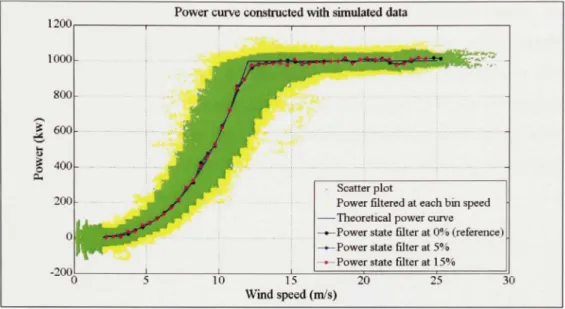
They also have proved that the Markov power-curve, which is the red curve in Figure 1.5, isn't affected by the turbulence intensity, which is not the case with the lEC standard. Figure

1.5 shows also that the lEC power curves are affected by the turbulence intensity (0, since the rated power is decreasing when the turbulence intensity is increasing. Moreover, in this graphic the Markov power-curve does fit exactly the theorefical power curve, which is not shown but explained by the authors of [7].

L(uVLni,Bd 80 40 u[m/sl ^5TrH!»WKW"»" — Mu ) - IEC(i;=5% ) - - - IEC(e;=15 % — IEC(C=25» i 20

Figure 1.5 Power curves obtained for a simulated data set [7].

The explanation of the literature review was necessary in order to introduce the subject analysed in this thesis. This chapter explained the standard method, the flaws of this method, the introducfion of the Markov's theory, and also some works done by GE and the University of Oldenburg. With all these elements, it is now possible to look at the mathemafical model of the Markov's theory, by applying Langevin equafion.

CHAPTER 2

MATHEMATICAL MODE L

2.1 Langevi n equatio n for Brownian motio n

In statistical physic, a Langevin equation is a stochastic differential equation describing a simple and well known Brownian motion in a potential [18]. Consequently, before analysing a Langevin equation, we will first discuss the Brownian motion of particles in its simplest form. A Brownian motion is a random movement of particles suspended in a fluid and it is also called a Wiener Process [16]. If a small particle is immersed in a fluid, then a friction force will act on the particle. The Stoke law gives the equation for this damping force [15].

Fc =-y^v (2.1 )

Also the Newton second law express that the summation of forces on an object is equal to the mass of this object muhiphed by his acceleration.

1'^=

Therefore, the expression of motion for the particle of mass (m) without any additional forces is given by:

mv + Xv = Q .23)

and the relaxation time (T) is defined as:

r = ^ (2.4)

However, this equation is valid only when the mass of the particle is large enough so its velocity due to thermal fluctuations is null or negligible. The mean energy of the particle in one dimension is given by the equipartition law [17]. The original concept of equipartifion was that the total kinetic energy of a system is shared equally among all of its independent part once the system has reached thermal equilibrium [17].

^m{v') = hj (2.5)

The equation (2.3) needs to be modified with the respect of equation (2.5), which leads to the correct thermal energy. The correction consists in adding, on the right-hand side of (2.3), a fluctuating force (Fj), which is a stochastic or random force [15].

F(t) = F^{t) + F^(t) (2.6) The fluctuating force occurs because the problem isn't treated exactly. If the problem was

treated exactly, the coupled equations of motion for all the molecules of the fluid and for the small particle would be solved, and then, no stochastic force would occur. In reality, because of the large number of molecules in the fluid (in the order of 10^^), these coupled equations generally can't be solved.

Therefore, the force (Fj) varies from one system to the other, and one thing to do is to consider the average of this force for the ensemble. The fluctuating force per unit mass (F), which is called the Langevin force, is obtained by dividing the force (Fj) by the mass. We also divide all the remaining terms of the equation (2.6) by the mass and we thus obtain the equation of the Langevin force.

20

The first assumption of this force is that its average over the ensemble should be zero, since the equafion of motion for the average velocity is given by the equation (2.3).

( r ( r ) ) - 0 (2.8)

If two Langevin forces at different times are multiplied, we then assume that the average value is zero at time differences (t'-t), for a time larger than the duration of a collision (TQ). This assumption seems to be reasonable, since the collisions between the molecules of the fluid and the particle are approximately independent.

{r{t)rit')) = o

fo r \t-t'\^T^i

Nevertheless, the duration time of a collision is usually much smaller than the relaxation time (T) of the velocity of the particle. Therefore, the limit of TQ ^ 0 should be taken as a much more reasonable approximation.

{r(t)r(t')) = qS{t-t') (2.10) Risken describes in reference [15] the apparition of the delta (S) function. He states: "The 5

function appears because otherwise the average energy of the small particle can't be finite as it should be according the equipartition law" shown at the equation (2.5). The variable (q) describes the noise strength of the Langevin force. In fact, the noise strength is the variable which describes the size of the scatter plot. More the strength is high, more the scatter plot will be large.

q = 2AkT/m^ (2.ii) Once the Brownian motion is explained, the Langevin equation can be introduced. The form

c^h(c,t)+g(c,t)nt)

(2.12

)

The noise strength may be absorbed in the function g, while the fiinction h is the deterministic drift. Also, the Langevin force is again a Gaussian stochastic variable with zero mean and delta correlated fiinction. However, a formal general solution for the stochastic differential equation (2.12) can not be given [15].

2.2 Fokker-Planc k equation

The introduction of the Fokker-Planck equation is necessary to better understand the origin of the equations and variables, which will lead to constmct a power curve following Markov's theory.

The probability density of the stochastic variable can be calculated with the Fokker-Planck equation. The Kramers-Moyal expansion coefficients of this Fokker-Planck equation are giving by [15]:

Therefore, the solution of (2.12) is giving by C (t + r) where r > 0. The differential equafion (2.12) is then written in the form of an integration to derive these Kramers-Moyal expansion coefficients.

at+r)-x= \[h(at'),t')+g(aannn]dt'

(2.i4

)

After some manipulafions of the equation (2.14), giving by [15], and with the limit x —> 0 we thus obtain for the drift coefficient:

D^\x,t) = h(x,t) + ^^g(x,t) (215) dx

22

The term D ' ' contains the deterministic drift and another term which is called the noise-induced drift.

^ : i - , w = ^ ^ ( x , 0 = {|-^<^'(x,0 (2.16)

ax 2 ax

2.3 Stochastic processes

Let's start the stochastic processes by defining that the probability that the random variable C is equal or less than x is called Q (C'^x). Since the variable Cis also real, then Q (CS '^) = \. Therefore, the derivative of Q with respect to x is the probability density function (W) of the variable C

W^(x) = j-Qi^<x) = {S(x-^)) (2-17) Also, by assuming that Q is differentiable, the probability dQ to find the continuous

stochastic variable ^ in the interval (x < C<x + dx) is seen as follow:

Q{^<x + dx) -Q(^<x) = — Q(^ < x)dx = W, (x)dx (218) dx

The probability density of the random variable C at time /„, under the condition that the random variable at the time /„-! < /n has the sharp value Xn-i, is defined by the conditional probability density.

Q(Xn^t„\x„_„t„_,',...',X„t,) = {S(X„-^(t„))) I _{|(r„-l)=x„-l ^(r|)=x ,}

2.4 Marko v property

A Markov process is a type of stochastic process. The process described by the Langevin equation (2.12), with 8-correlated Langevin force, is a Markov process. Its conditional probability at time t^ depends only on the value at the next earlier time. However, if r(r) is no longer (5-correlated, the Markov property is destroyed.

2(^„.'J-Vi.'„-i;-;^p^i) = 2 ( ^ „ ' ' J ^ « - i > d ) (2.20)

The interpretation of equation (2.20) may lead that there is only a memory value of the variable for the latest time. The arbitrary of the time difference /2 - 'i of the conditional probability Q(x2,t2\x\,ti) of a Markov process, affects the dependence of Q on xi. Indeed, if the time difference is large, then the dependence will be small, conversely if the time difference is infinitesimally small then the conditional probability will have the sharp value xi [15]. If n = 2 and the time difference is infinitesimally small, then the conditional probability will be giving by:

limQ(x^,/j I X,,?,) = S(xj -Xj) (221)

2.5 Coefflcient s estimatio n

As seen in (2.13), the Kramers-Moyal expansion coefficients of the Fokker-Planck equation are giving by:

D<"»(.T) = - l i m - M ' " ' ( x , r ) (2-22)

n\ '•^ 0 T

with the conditional moment (A/ ')

24

Now the variable x can be replaced by Psiaie, which is the power state in a certain bin speed, while X, can be replaced by P which is the power output of the wind turbine. In fact, there are multiple power states inside a certain bin speed.

^ r (P.a,e > r) = {P(t + r) - />(/)>! ,„^^ (2.24)

The expected power output of Pstaie is then calculated with the conditional probability density Q(P„+\, t + x\P„, t). This conditional probability describes the probability of states Pn+\, of the system variable Psiate, at time t + x with the condition that the system is in state P„ at time

t[\].

The drift coefficient (D*'') is then obtained by dividing the conditional moment (M) by the relaxation time (T) and then calculating the limit r —> 0. The drift can be explained as a force that acts on each power state inside a bin speed and it is directed toward the stationary power at this bin speed. For example, if we have a strong negative force, then the power state where the calculation has been done is much higher than the stationary power. On the other hand, if we have a small positive drift, then the power state is a little bit smaller than the stationary power.

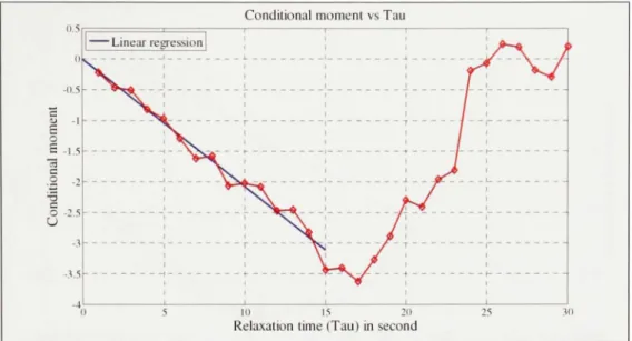
In order to calculate the drift coefficient, it is necessary to calculate the slope for an interval of r where we assume the process to be Markovian [7]. The Figure 2.1 shows an example of the conditional moment in function of the relaxation time at a certain power state. Therefore, the drift coefficient is the slope of the linear regression.

; . ( l . ( n .dM^^'iP...,^)

Conditional moment vs Tau •il5 -2..S 1 Linear regression | 1- 1 — - - t — / 10 I Relaxation time 5 2 0 (Tau) in second

Figure 2.1 Example of conditional moment in function of the relaxation time (r).

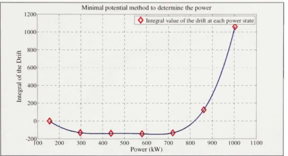
Then, the stationary power is found by the search of null crossing or the minimal potential of the deterministic coefficient D^^\Pstate) [!]• The stationary power found with the minimal potential is defined as:

C,™,n=min(-JD'"(/'_)^P,„J

Even if the search of zero crossing seems easier, the minimal potential doesn't cumulate errors like the fit of the linear regression. In fact, if there is a drift value which is offset of its supposed value, then the linear regression will fit to that error, while the minimal potenfial will be less affected. Therefore, theoretically this method is more accurate. As shown in Figure 2.2, and explained in thesis of GE's student [13], the minimal potential and the linear regression do not give the same result when calculating the stationary power at a certain power state.

26 s 2 8 .0 1 Drif t 3e 6 9 '% -n « -• *^-^ 1 " • - - ^ ^^* _{^ ^ •}

^V- •

Figure 2.2 Comparison of the minimal potential with the zero crossing to

determine the stationary power output [13].

With the mathemafical model presented in this chapter, which contains the methods to calculate the conditional moments, the drift coefficients and the stationary powers, we will calculate the Markov's power curve, and analyse the impact of different parameters. This analysis will be shown in Chapter 4 for the MM anemometer and Chapter 5 for the nacelle anemometer. However, before doing any analysis, we will first introduce the turbine analysed in this thesis.

WIND-TURBINES DESCRIPTION

The data analysed in this thesis are all supplied by the wind-energy division of General Electric (GE). Those data are also from GE's wind turbines. GE is one of the world leaders in manufacturing and assembly wind turbines, with more than 7500 turbines installation, which produce more than 9800 MW [4].

Prior to constmction of a power curve following Markov's theory, we will describe the wind turbines to analyse. In this thesis there will be three wind farms and five wind turbines to evaluate. In this chapter the introduction of those wind mrbines is done. This includes the description of the turbines, the MM anemometer, the wind measurement sectors, the scatter plot of the power in fiinction of the wind speed, the location of those wind farms and more.

3.1 Klondike-I I

The Klondike-II site is located in the U.S.A. in Oregon state (see Figure 3.1). It has 50 mrbines, which generate a total 75 MW of wind power, including one 1.5xle and forty-nine 1.5sl. The turbine model analysed in this thesis will be the 1.5xle and it produces 1,5 MW at the rated wind speed, which is reached at 12,5 m/s. The cut-in wind speed of this turbine is 3,5 m/s, while the cut-off wind speed is 20 m/s. The rotor speed is variable, (between 10,1 and 18,7 rotation per minute (rpm)) and its diameter is 82,5 meters. The electrical frequency output of this turbine can be either 50 Hz or either 60 Hz to accommodate European and North American standard respectively.

The output power of the turbine is recorded by a measurement system at a rate of 50 times per second. The data analysed in this thesis was obtained over a three weeks period from Febmary 5"* to Febmary 28"^ 2006. The anemometers for Klondike-10 are both Sonic for the

28

MM anemometer and for the nacelle anemometer. For the MM anemometer it is a Gill Windmaster P6032, while for the nacelle anemometer it is a Metek USA-1.

Figure 3.1 Klondike-II site located in U.S.A. in the Oregon State.

For the Klondike-ll site, the turbine analysed will be Klondike-10. This turbine is situated at a distance of 197 meters of the meteorological mast. The wind measurement sector is between 236 and 315 degrees. The scatter plot of the power in funcfion of the wind speed is shown at Figure 3.2.

1800 1600 1400 1200 Powe r (kw ) 400 200

°(

Scatter plot of ttie power in function of the wind speed for Klondike-10

''^'W^^^^^KB^''^''--'' ml^^^P^' • .T'OSBBK} ••'ilK^KI^^ " ) 5 1 0 1 5 2 0 Wind speed (m/s) -2 5

Figure 3.2 Scatter plot of the power in function of the MM wind speed at an

averaged time of 1 second for Klondike-10.

3.2 Wietmarsche n

The Wietmarschen site is situated in Germany (see Figure 3.3). ft is composed of mulfiple 1.5sl turbines, which produces 1,5 MW of wind power at a rated wind speed of 14 m/s. The cut-in wind speed of those turbines is 3,5 m/s, while the cut-off wind speed is 20 m/s. Like Klondike-II turbines, the rotor speed is variable. In fact, it varies between 11 and 20,4 rpm and its diameter is 77 meters. The electrical frequency output of this turbine is 50 Hz, which can not be utilised in North America.

The output power of the Wietmarschen turbines is recorded at a rate of 50 times per second. The data analysed in this thesis are obtained on a 19 days period, which was collected in December 2004. The anemometers for both Wietmarschen turbines are Sonic, while it is also the same for the MM anemometer. All anemometers do have a Gill Windmaster 1086M. The Wietmarschen turbines do also have a cheap cup anemometer at the nacelle, but we won't ufilise the data obtained from this anemometer in this thesis, since it is not as accurate as the Sonic anemometers.

30

Figure 3.3 Wietmarschen site located in Germany.

For Wietmarschen site, the turbines analysed will be Wietmarschen-1 and Wietmarshen-2. Those turbines are at a distance of 269 and 185 meters respectively of the meteorological mast. The wind measurement sector for both turbines is between 218 and 318 degrees. The scatter plot of the power output in funcfion of the wind speed, for the Wietmarschen-1 turbine, is shown at Figure 3.4. It can be noticed that the scatter plot is much larger for Klondike-10 turbine. Therefore, the Markov's theory will be tested, because it will be interesfing to study the behaviour of the power curve when the turbulence intensity is much larger than usual. This effect has been shown at Figure 1.5, when the lEC power curves were constructed at different turbulence intensity.

Scatter plot of the power in fiinction o f the wind speed for Wietmarschen-1

10 1 5

Wind speed (m/s)

Figure 3.4 Scatter plot of the power in function of the MM wind speed at an

averaged time of 1 second for Wietmarschen-1.

3.3 Pretti n

The Pretfin site is situated in Germany (see Figure 3.5). The turbines ufilised for this site are the same as the Wietmarschen-site ones (1.5sl turbines). All the parameters of Pretfin-site turbines are the same than the ones of Wietmarschen-site turbines. Unlike Wietmarschen and Klondike turbines, the output power of Prettin turbines is recorded at each second. The data analysed in this thesis are obtained over a 5 months period and was collected from June to November 2006. The anemometers for both Prettin turbines are the same than the ones from Wietmarschen turbines. Thus they are all Sonic anemometers of type Gill Windmaster

1086M. Also, like the Wietmarschen turbines, the Prettin turbines do have a cheap cup anemometer at the nacelle, which we won't ufilise in this thesis.

32

Figure 3.5 Prettin site located in Germany.

For Prettin site, the turbines analysed will be Prettin-4 and Prettin-5. Those turbines are at a distance of 369 and 291 meters respecfively of the meteorological mast, which is a long distance. Indeed, the locafion of the MM shouldn't be beyond four times the rotor diameter, which is 308 meters in this case. However, this long distance will test the Markov property, since the correlation between the wind speed read at the MM anemometer and the power output at the turbine will be reduced. Therefore, the scatter plot will be larger and the turbulence intensity will increase.

The wind measurement sector is between 207 and 256 degrees for Prettin-4, while it is between 210 and 305 degrees for Prettin-5. The scatter plot of the power in funcfion of the wind speed, for the Prettin-5 machine, is shown at Figure 3.6.

1800 1600 1400 1200 ^.^ er(k w ₈ 5 800 o (X, ₆₀₀ 400 200 Q

Scatter plot of the power in function of the wind speed for Prettin-5

1 1 1 1 . rJd:r"^£n^^r^-^^^'^^':'-i!i'.^^AJ/' > •"•

-'.^^^HHHHHR^f^v!TT^ •

y>-(J^^^^^^HPP^' y^'

Figure 3.6 Scatter plot of the power in function of the MM wind speed at an

averaged time of I second for Prettin-5.

Now, we do have a good idea of the turbines utilized in this master thesis, and we do know the differences between the equipments on each wind farms. The main difference is the measurement system of Klondike-10 and Wietmarschen turbines, which is not the same than Prettin turbines, since it can only collect the data once per second, while it is 50 times per second for the three others turbines. The data obtained from these equipments will be ufilized to optimize the Markov power-curves by evaluafing the effect of different parameters.

CHAPTER 4

POWER CURVE CONSTRUCTED WITH THE METEOROLOGICAL-MAS T ANEMOMETER

Before constmcting a nacelle power-curve following Markov's theory, it is preferable to make it with the MM anemometer, since the wind speed isn't affected by the blade passage. Moreover, it is also important to constmct a power curve with the simulated data, because as shown in secfion 1.2, the stochastic power curve will not fit with the lEC power curve, so there won't be any reference to know if the Markov power-curve software is working or not. However, if simulated data are created following a theoretical power curve, like illustrated in Figure 4.1, then it will be possible to validate if the software and the novel theory are good to constmct a power curve. Thus, knowing that the software is good, the power curve made with real data will likely be good.

In a perfect Markov power-curve we want to have a perfect cubic curve, which start from the cut-in wind speed until the rated power. This means if the curve constmcted with Markov theory doesn't follow perfectly a cubic curve, then the Markov power-curve isn't considered perfect. From the rated wind speed the curve should become horizontal until the cut-off wind speed. In fact, the theoretical power curve shown in Figure 4.1 is a good example of what we want to look for in a perfect Markov power-curve.

Scatter plot of the simulated data around the theoretical power curve 1000 800 I 600 I 40 0 a. 200 -200, 1 1 1 I 1 f .Wfc r . .-.v-o*. ' • P - .J' ••• -r—^'^ Scatter plot Theoretical i 1 m^^tiX'^rf^rrr^ 0^^fK.-f- •••

of the simulated data power curve

10 1 5 2 0

Wind speed (m/s)

25

Figure 4.1 Scatter plot of the simulated data around the theoretical power-curve [6]. However, mulfiple differences are present between the real and the simulated data. The first difference is that the wind speed read at the meteorological-mast anemometer takes a certain fime before reaching the turbine. Moreover, the wind turbine doesn't react instantly to the wind speed fluctuation. In order to solve the turbine reaction, it is necessary to take a relaxafion time (r), for which the values will give an appropriate linear regression in the calculation of the drift, like shown at the Figure 2.1. The relaxation time used in this thesis, is between 5 and 15 seconds, according to the research made by the University of Oldenburg [8]. In this report, we assume that the simulated data react the same way than the turbine. In fact, by making this supposition the software utilised to calculate the Markov power-curve is the same for real and simulated data.

Another difference is the apparition of holes when utilising the real data. Indeed, those holes are created either when the data at a certain moment aren't good, or when there is a period of time, more than the relaxation time, between the data recorded. The bad data appear because either the system of the turbine is malfuncfioning, the wind speed is outside of the measurement sector, or there is a sensor that is not working properly or other different reasons. Nevertheless, Markov's theory doesn't accept those holes in the data, since the

36

calculation of the moment needs to be done with the respect of the equation (2.24), in which the power differences need to be taken at each relaxation time.

To lighten the report, only the power curves from the simulated data and Klondike-10 turbine are presented in graphic form. However, the analyses are also done for the four others turbines. The final results of the power curve for those turbines will be presented in the Chapter 6 to verify Markov power-curve efficiency.

4.1 Defaul t power-curve

To start the analysis, we will set a default power-curve. This default power-curve can be modified in further section depending on results obtained. Therefore, if we find out that parameter A is better than parameter B, then parameter A will be kept in all fiarther sections of this thesis. For the moment, the default power-curve is constmcted with:

> the mean to calculate the conditional moment;

> the minimal potential to calculate the stationary power; > ten power states at each bin speed;

> the relaxation time constant between 5 and 15 seconds; > the bins speed set at 0,5 m/s;

> the averaged fime of the data at 1 second.

The flowchart of the Markov power-curve software is shown in the APPENDIX I. Figure 4.2 and Figure 4.3 illustrate the default power-curve for the simulated data and for the meteorological-mast anemometer of Klondike-10 respectively. The power curve constmcted with the lEC standard, for the simulated data, is well under the theoretical one at the rated power, while the one made with the Markov's theory is much closer. This demonstrates the flaw, explained in section 1.2, of averaging instead of taking the stationary power. The power curve obtained for Klondike-10 with Markov's theory is obviously not good. Indeed, the power found at the bin speed of 6,25 m/s is too high of what it was supposed to be. In fact.

the power curve needs to follow a cubic curve before the rated power. Moreover, once the power curve has reached the rated power, the power curve following Markov's theory stops, which is another sign of bad power curve.

1200 1000 800 I 60 0 I 40 0 200 -200,

Power curv e constructe d wit h simulate d dat a

if"

Scatter plot of the simulated data Theoretical power curve —•—Markov power curve

E C power curve

-1 1 1

10 1 5 2 0

Wind spee d (m/s ) 25 30

Figure 4.2 Default power-curve for the simulated data.

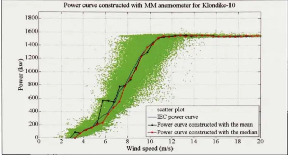
Power curv e constructe d wit h MM anemomete r fo r Klondike-1 0 1800 1600 1400 ^ 1 2 0 0 '^lOOO Urn u I 80 0 600 400 200 0 0 MflWiiMMi scatter plot

TEC power curve

—•—Markov power curve

8 10 i : Wind spee d (m/s)

14 16 18 20