Detection of core-collapse supernovae through joint analysis of LIGO gravitational wave and KamLAND neutrino data

(1)

Detection of Core-Collapse Supernovae Through

Joint Analysis of LIGO Gravitational Wave and

KamLAND Neutrino Data

M

by

Emmett E. E. Krupczak

Submitted to the Department of Physics

in partial fulfillment of the requirements for the degree of

Bachelor of Science in Physics

at the

MASSACHUSETTS INSTITUTE OF TECHNOLOGY

ASSACHUSETTS INSTITUTE OF TECHNOLOGY

JUL

0 7 2016

LIBRARIES

February 2016

@

Massachusetts Institute of Technology 2016.

Author

Signature redacted

Author .

All rights reserved.

Department of Physics

Jan 4, 2016

Signature redacted

Certified by

...

Professor Lindley Winslow Thesis Supervisor

Accepted by ...

Signature redacted...

Professor Nergis Mavalvala Senior Thesis Coordinator, Department of Physics

(2)

(3)

Acknowledgments

I gratefully acknowledge the support of my advisor, Lindley Winslow. I am deeply thankful for her guidance and encouragement. I would like to thank Erik Katsavouni-dis and the LIGO scientific collaboration for generously taking the time to answer my questions, and for providing me a sample of LIGO's data. I am immensely grateful to Koji Ishidoshiro and the KamLAND collaboration for granting me access to the neutrino data and advising me on all aspects of KamLAND. I am greatly apprecia-tive to the KamLAND collaboration members at the Research Center for Neutrino Science at Tohoku university for their wonderful hospitality. Thank you also to the Gravitational and Neutrino Working Group. Finally, I thank Peter Schmidt-Nielsen for programming advice and assistance with the figures.

(4)

(5)

List of Figures

4-1 Schematic of KamLAND Detector . . . . 26

4-2 Distribution of prompt and delayed energies for candidate C/e events. 28

4-3 Supernovae neutrino energy spectrum . . . . 29

4-4 Distribution of > 7.5 MeV neutrino events in the KamLAND detector volum e. . . . . 30

4-5 Candidate KamLAND neutrino events . . . . 30

4-6 Energy distribution of candidate neutrino events above 7.5 MeV thresh-o ld . . . . 3 1 5-1 Time between subsequent KamLAND neutrino events with energy

above 7.5 M eV . . . . 38

5-2 Time of sample gravitational event and candidate neutrino event . . . 39

(8)

(9)

Chapter 1 Introduction

Core collapse supernova are one of the most intriguing astrophysical phenomena. The dying stage of a supergiant star, they occur when the star collapses into a proto-neutron star, causing a shock wave and a gamma ray burst. High energy neutrinos are released in this process and offer the possibility of detecting these elusive cataclysms. The number of neutrinos emitted is large but at best only a few will be detected. With a multi-messenger search, we can combine the neutrino signal with another clue to the presence of a supernova: gravitational waves. During the proto-neutron star stage, a fast-rotating star can produce gravitational waves via its asymmetric and rapidly shifting mass. By combining the signals from neutrinos and gravitational waves, we can attempt to detect supernova signals that are too faint to detect alone. Joint searches have already been attempted by several neutrino experiments with high-energy thresholds, including ANTARES and IceCube. This thesis explores the possibility of a joint search with a new set of neutrino data. KamLAND (Kamioka Liquid scintillator Anti-Neutrino Detector) is a large particle detector located in Kamioka, Japan. KamLAND is well-shielded, with an low (~ 1 MeV) energy thresh-old and has more than ten years of data to explore, making it a good candidate for a joint search. A recent search of KamLAND's data for clustered events indicative of supernova found no clear clusters. A new search is needed to identify single-neutrino events that may have originated in supernovae. A joint search will help KamLAND more carefully examine the possible sources of its single-neutrino events.

(10)

The gravitational wave data comes from LIGO (Laser Interferometer Gravitational wave Observatory). Located in Hanford, WA and Livingston, LA, LIGO consists of two four-kilometer interferometer arms. Analysis of LIGO data from 2005 to 2010 did not produce any clear gravitational wave events, leading to a need for a more sensitive search. A multimessenger search in conjunction with KamLAND provides this opportunity. We can examine both KamLAND and LIGO's data in order to search for possible supernova signals observed by both experiments. Because a joint data-sharing agreement has not been reached between KamLAND and LIGO, this thesis looks at the potential of a joint analysis and the opportunity for such a study

(11)

Chapter 2 Core-Collapse Supernovae

The violent demise of massive stars leads to the aptly named phenomenon of a su-pernova. Having an accurate picture of supernovae is essential to our understanding of astrophysics. Supernovae hold crucial information for describing all aspects of star formation and lifetimes, including star formation, stellar evolution, and stellar popu-lation synthesis [2]. The chemical composition of galaxies is dictated by supernovae; they provide the interstellar material and disperse the heavy elements that later come to comprise solar systems, planets, and all their inhabitants. Even the elements in our blood have their origins in supernovae.

In order to understand supernovae, we must probe them using whatever detectable clues are available to us. We will focus on the major class of supernovae known as core-collapse supernovae. The likely signatures of a supernova are neutrinos and gravitational waves, which can be seen by examining the mechanism by which core-collapse supernovae are produced.

2.1 Mechanism of Core-Collape Supernovae

Core collapse supernovae originate from the death throes of supergiant stars. The power in a star is generated through nucleosynthesis as each successive element un-dergoes fusion. First, the star begins by burning hydrogen. As hydrogen gives way to helium, the core becomes hotter and more massive, until the hydrogen is exhausted

(12)

and the helium fusion begins, fusing the helium into carbon and oxygen [3]. For main-sequence stars, this is the final stage: once the core is entirely comprised of oxygen and carbon, no further fusion can take place. These stars will eventually eject their outer layers as planetary nebula and retire into white dwarfs

[4J.

For high mass stars such as supergiants, however, the stars are massive enough to continue fusion beyond carbon and oxygen. The gravitational pressure exerted on the cores of supergiant stars of eight solar masses or greater is sufficient to fuse carbon into sodium, neon, and magnesium [3]. Once all the carbon has been exhausted, photodisintegration can create new helium nuclei. These helium nuclei can then fuse to the existing elements to create yet heavier elements; for example, photodisintegration can turn neon into magnesium via the following mechanism [3]:

S+20 Ne - 16 0 +4 He

4_He

+20 Ne _{-+24 Mg}

As each subsequent element is exhausted, the core contracts, increasing the tem-perature enough to produce the next element. This is the same cascade witnessed in the trajectory of main-sequence stars, but supergiant stars can carry the chain much farther. Once the neon has been exhausted, core contraction and heating cause oxygen to fuse into silicon. The silicon then can undergo photodisintegration and subsequent fusion to reach sulfur. By this mechanism, argon, calcium, chromium, manganese, iron, cobalt and nickel can all be produced. Ultimately, the silicon in the core is entirely converted into iron

[3].

The immense gravitational pressure is now countered entirely by the electron degeneracy pressure.

As a supergiant star approaches the Chandrasekhar mass, gravity becomes stronger than the pressure of degenerate relativistic electrons. This forces the electrons into the nucleus where they are captured by protons, creating neutrons and releasing electron neutrinos [2]:

(13)

The gravitational collapse begins to trap the neutrinos produced by electron capture when the timescale of core collapse becomes shorter than the timescale for electron neutrino diffusion out of the core. Instead of diffusing out of the collapsing core, the neutrinos coherently scatter off the iron nuclei [5]. Neutrinos are also generated through electron-positron pair annihilation [6]. This further decreases the electron pressure, and the process continues until an equilibrium is reached between gravity and the outward pressure exerted by the nuclear forces between neutrons, creating a proto-neutron star [2].

The collapse process undergone by the supergiant star causes the stellar core to shrink from a radius of ~ 1500 kilometers to a few tens of kilometers in less than half a second. As the core collapses, the gravitational energy is transferred to the stellar envelope, which reverses the infalling motion and creates an explosion [2]. The matter in the stellar envelope ends its free-fall by bouncing inelastically against the core. This bounce occurs when the nuclear densities reached in the collapsing core are such that the the repulsive nuclear forces dominate (5]. The bounce transfers kinetic energy into the iron nuclei, causing the iron nuclei to dissociate into free nucleons [2]. This collapse and bounce of the iron core causes a strong shockwave.

The electron capture process generates a large amount of electron neutrinos just behind the shockwave front [5]. The electron neutrinos have a very long diffusion time because they are trapped by an opaque region behind the shockwave; as a result the shock propagation occurs on a much faster time scale than the diffusion of neutrinos. The electron neutrinos are thus largely unable to escape until the shockwave reaches the neutrino sphere. As the shockwave reaches the neutrino sphere and passes through it, it causes the electron neutrinos to abruptly decouple from the matter of the star and propagate ahead of the shock wave. This creates the "breakout" burst, which releases a huge number of electron neutrinos; the peak luminosity is 1053 ergs per second and the duration of the burst is about 20 milliseconds. It is this burst of neutrinos which create the signal that neutrino observatories hope to detect [5].

The high neutrino flux exiting the supernova carries away the majority of the grav-itational energy gained during the contraction phase. The energy of the shockwave is

(14)

further absorbed by the nuclear dissociation of the iron nuclei and electron capture. This causes the shockwave to stall

[7].

At this point, there are two possible outcomes: black hole or supernova. If the shockwave remains stalled, the supernova will fail and the proto-neutron star will continue to accrete, eventually becoming a black hole [7]. This occurs in a significant fraction of stars. The "mass gap" between the heaviest observed neutron stars and the lightest black holes is caused by this threshold be-tween stalled shockwaves and completed supernova. Analysis of this mass gap allow the determination of the timescale on the collapse occurs. Current evidence indicates that core collapse supernovae are launched within 100-200 milliseconds of the initial stellar collapse [8].

If the shockwave breaks out of the stall, the result will be a core-collapse supernova.

The shockwave stall can be overcome by neutrino heating. Just after the stall begins, the area between the protneutron star and the stalled accretion shock enters quasi-hydrostatic equilibrium. The core of the proto-neutron star is very hot and very dense and produces a large number of neutrinos. The proto-neutron star has a very large amount of gravitational binding energy which is carried to the shock front by the neutrinos. If the neutrinos transfer sufficient energy to the stalled shock front, this will re-ignite the explosion and lead to the supernova [5].

The re-energized shock wave will enter the stellar envelope and break through the photosphere, causing the supernova explosion. While some energy is lost to neutrino dissipation and photodissociation when passing through the stellar envelope, it is a negligible amount and is not enough to circumvent the explosion [5]. The supernova flings off the outer layers of the star, scattering the fused elements into the interstellar medium. The supernova remnant disperses over the following hundred thousand years [9].

The Milky Way galaxy produces only a few supernovae per century. The frequency of core collapse supernovae within 10 megaparsecs of Earth is expected to be a few per year, coming from many surrounding Milky Way-like galaxies, as well as several galaxies with unusually high predicted supernova rates [10]. The rarity of these supernovae requires us to make every effort to detect even the more distance events.

(15)

2.2 Neutrinos from Core-Collapse Supernovae

The burst of neutrinos released when the shockwave passes through the neutrino sphere signals the birth of a black hole or a core collapse supernova [10]. These high-energy neutrinos are produced by proton-photon (py) reactions when Fermi-accelerated relativistic protons interact with high energy outflow photons to create pions or kaons [11]. Fermi acceleration is the acceleration experienced by charged particles when they are repeatedly reflected. The particles do not collide with other particles directly; instead, they "bounce off" a magnetic field [12].

Fermi acceleration requires an inhomogeneous magnetic field. A propagating shockwave, as is produced by a core-collapse supernova, tends to produce such a magnetic field. When the charged particle encounters a moving change in the mag-netic field, it is then reflected back through the shockwave. Each time the particle is reflected, it gains energy. By bouncing back and forth between the magnetic fields traveling with the shock front, particles can reach very high speeds [12]. These high speed protons then combine with photons produced by the gamma ray bursts in the supernova. The p-y reactions consume a significant portion of the gamma ray burst energy, transforming it into neutrinos of about ~ 10" eV. The gravitational energy release transferred to neutrinos is about 3 x 101 ergs, about 100 times more than the kinetic energy required for the explosion [10].

Once the protons and photons have created a meson, the meson then decays and

produces neutrinos. For example, the dominant decay pathway for a lr+ is:

7r + It++V -+ e+ +e +VL + V,

These decays could produce a neutrino-antineutrino pair of any generation; the ratio of electron to muon to tau is approximately 1:2:0. Due to flavor oscillations, this ratio becomes approximately 1:1:1 by the time the neutrinos reach Earth [11].

These neutrinos provide the most promising source of information about core-collapse supernovae, and consequently detecting them is of the upmost priority. This, however, proves very challenging. A supernova will, at best, provide only a few

(16)

neutrino events, making it hard to compare data to predictions from models. The best-characterized supernova to date, SN1987A, only provided about 20 detected events [10]. Therefore, increasing our sensitivity to supernova neutrinos is a top priority.

2.3 Gravitational Waves from Core-Collapse

Super-novae

Core-collapse supernovae produce gravitational waves at each stage of development. Any instability in the rotating star which causes a changing and asymmetric mass can produce gravitational waves, but the majority of the gravitational waves from core-collapse supernova originate from the initial core-collapse and the core bounce. The initial collapse produces gravitational waves as the quadrupole moment of the star changes. During the initial collapse, the quadrupole moment of the star changes. Einstein's quadrupole formula for gravitational radiation states that the wave amplitude of the gravitational wave is proportional to the second derivative of the source's quadrupole moment. The frequency and amplitude of the emitted gravitational wave can be used to calculate the radius and mass of the source; for example, a black hole or a neutron star [13]. The luminosity of gravitational waves of a given source is given by:

LW C' (Rsch )2 (V)2 LGW

G R c

where R is the radius of the source, Rsch is the Schwartzchild radius, and v is the velocity of the components of the system [13]. The amplitude of the gravitational waves at a distance r from the source is roughly given by:

h(r) ~G Ek

C r

where Ekin is the kinetic energy of the source and 0 < c < 1 is the fraction of kinetic energy that is available to produce gravitational waves. The factor c indicates the

(17)

asymmetry of the source. For example, in a spherically symmetrical explosion, 6 = 0

and thus no gravitational waves will be produced. Only a time-varying quadrupole moment produces gravitational waves [131. The quadrupole moment varies in a dif-ferent way for core-collapse supernovae, neutron stars, and black holes, producing a unique gravitational wave signature that can tell us the path the dying star followed. The initial signal is caused by the changing axisymmetric quadrupole moment pro-duced during the collapse of the supergiant star. When a neutron star forms, the quadrupole moment increases as the star contracts. When a black hole forms, by contrast, the quadrupole moment increases initially but then dramatically decreases

[13].

The other source of gravitational waves from a core-collapse supernova comes from the core bounce. The infalling envelope bouncing against the core causes

axisymmet-ric normal mode oscillations if a proto-neutron star is created. These vibrations

can last for hundreds of oscillations. A black hole, rather, is excited in its

quasi-normal modes and the oscillation dies out after only a few oscillations. Rotating proto-neutron stars can produce additional gravitational wave signatures [13].

(18)

(19)

Chapter 3 Past Supernovae Searches

3.1 Neutrino-only supernovae search

A supernova search was done using just KamLAND neutrino data 114]. The neutrino

events selected overlap with the events that were considered in this study: neutrinos of an energy range between 7.5 MeV and 30 MeV, that took place between 9 March 2002 and 14 June 2012. Selecting for the best data-collection runs leaves a live time of

6.5 years during this ten-year interval. Twenty-nine neutrino events of the appropriate

energy occurred within the selected interval. A supernova event was considered to be a burst of two or more 1e delayed coincidence event pairs within 10 seconds [14]. No candidate supernova events were found. This was used to put an upper limit of

~ 0.36 events per year within ~, 70 kiloparsecs (CL 90%) [14].

3.2 Gravitational wave-only supernovae search

Several supernovae searches have been performed using only gravitational wave data.

LIGO has collaborated on these studies with the Virgo and GE0600 detectors. Virgo

is a 3 km long interferometer gravitational wave detector located near Pisa, Italy. Virgo has a seismic isolation system which allows Virgo to be more sensitive than

LIGO to low-frequency (< 40 Hz) signals [15]. GE0600 is located near Hannover,

(20)

Michel-son interferometer with two 600 m arms. Each arm is singly-folded, leading to a total optical length of 2400 m [16]. The data from GE0600 was held in reserve and used to follow up any detection candidates uncovered in the LIGO-Virgo analysis. A joint search between the LIGO, Virgo, and GE0600 collaborations combined data from November 2006 and October 2007. No plausible gravitational wave event candidates were found, leading to an improved upper limit on the rate of bursts: 2.0 events per year for the 64-2048 Hz range and 2.2 events per year for higher frequencies [15].

A second search combining LIGO and Virgo data between 7 July 2009 and 20

October 2010 spanned 207 days of observation time. It observed no candidate events beyond the expected background and the threshold false alarm rate and was able to improve the upper limit on strong gravitational wave bursts, giving an upper limit of

1.3 events per year [17]. It also placed limits on the rate density of burst sources [17].

3.3 ANTARES-LIGO-Virgo joint search

ANTARES(Astronomy with a Neutrino Telescope and Abyss environmental RE-Search) was an underwater high-energy neutrino telescope, located at a depth of 2475 meters on the sea bed about 40 km off the coast of Toulon, France. It is designed to detect neutrinos in the GeV - TeV range [11].

A multi-messenger search for supernovae was performed jointly by the ANTARES, LIGO, and Virgo collaborations. The ANTARES-LIGO-Virgo joint search

consid-ers gravitational wave data from January - September 2007. This time period of

ANTARES data collection included 216 high energy neutrino events which coincided

with the fifth science run of LIGO and the first science run of Virgo [11]. No signif-icant coincidence events were observed, but the collaboration was able to set a limit on the population of gravitational wave and high energy neutrino sources. The limit on the rate density of such sources was determined to be:

(21)

where T

b is the beaming factor (the ratio of the total number of sources to the number

of sources with jets oriented towards earth), V is the volume of universe probed by the analysis and Tb, was the duration of coincident observations. In the ANTARES-LIGO-Virgo study, Tob, ~ 90 days [11]. For long gamma ray burst sources, which includes core-collapse supernovae, this gives a rate-density limit of:

PGW-HEN b EGW -3/2X 102Mpc-3yr-1

W10-2MOc2)- _l/y

where EGW is the total energy in a narrow-band gravitational wave burst and MD is the solar mass [11].

The most "optimistic" limit on the energy of gravitational-wave emissions by core collapse supernovae cited by this study is EGW - Moc2. This gives a rate limit of

[11]:

PGW-HEN b 2 -/2 X

10Mpc-3yr-- PGW-HEN Tb l5MpC yr

After correcting for beaming effects, the literature suggests a rate density limit for long gamma ray bursts of [18][11]:

Piong ~ 3 x 10- 8_{Mpc-3 yr-1}

And for short gamma ray bursts of [11]:

Pshort ~ 10 7MpC 3yr 1

Long gamma ray burst sources are closely related to Type II and Type Ibc core-collapse supernovae, which have local rates, respectively, of [111:

(22)

While the upper limit derived by the LIGO-Virgo-ANTARES study remain above these currently accepted source rates for both long and short gamma ray bursts, the maximum source density of ~ F10-5Mpc-3yr-1 derived using EGW ~ MOc2 is rela-tively close to these gamma ray burst source rates. The LIGO-Virgo-ANTARES study suggests that they only require a factor of two improvement in detection distance to begin constraining the fraction of stellar collapse events which produce coincident gravitational wave-neutrino signals [11].

3.4 IceCube-LIGO-Virgo joint search

IceCube is a cubic-kilometer Cerenkov neutrino detector located at the South Pole. IceCube is optimized to detect very high energy neutrinos, in the TeV to PeV range, but is also sensitive to MeV neutrinos, such as might be expected from a supernova. The detector is constructed from 86 vertical strings set into the Antarctic ice, each with a set of 60 digital optical modules which detect Cerenkov light from neutrino-induced charged particles [19]. IceCube collected data from 2007 to 2011, with dif-ferent numbers of strings deployed during difdif-ferent periods. The configurations that have deployment periods overlapping with LIGO's data-collection are: 22 strings from

2007- 2008, 59 strings from 2009-2010, and 79 strings from 2010-2011. These

collec-tion periods yielded 978, 3363, and 3892 neutrinos coincident with gravitacollec-tional wave data, respectively [19]. The LIGO-Virgo-IceCube study did not discover any suffi-ciently significant joint gravitational wave and neutrino events. No double-neutrino events that were coincident with a gravitational wave event were discovered, and the number of coincident single-neutrino events were consistent with the false alarm rate expected from background [19].

In the absence of any significant events, IceCube was able to find an upper limit on the astrophysical source rate. The LIGO-Virgo-IceCube study uses a different method than the ANTARES study. The effective detection volume is defined by the distance at which sources can be detected with 50% efficiency. The sensitivity of the search is determined in terms of the observed gravitational wave strain amplitude, h,,,, which

(23)

is dependent upon the isotropic-equivalent gravitational wave energy, EGW and the luminosity distance, D, of the source [19]:

kG1/2

hkGs ~2 -I 1(EGW) 1/2D-1 hrss '

r3/2

where k is a constant that is dependent on the polarization of the emission. This study chose k = V/15/8, which corresponds to a linearly polarized signal and is the

conservative estimate [19]. The false dismissal probability is then plotted in terms of h,ss; they find that for a false dismissal probability of 0.5, h,50 = 4.3 x 10-22 Hz"/2_.

Choosing a neutrino emission of E, = 1051 ergs and EGW = 10-2MGc 2, the upper

limit of source density obtained by this search is:

p = 1.6 x 10- 2_Mpc 3_yr-'

This upper limit is above the currently accepted source rate for core-collapse

super-novae, quoted to be ~ 2 x 10- 4Mpc-3yr~1. For a one-year observation period with advanced LIGO/Virgo and the full IceCube, the study projects an upper limit of 4 x 10- 4Mpc-3yr-1, which would put it within reach of the expected core-collapse supernovae rate [19].

The upper limits in core-collapse supernovae rates derived by the IceCube-LIGO-Virgo and ANTARES-LIGO-IceCube-LIGO-Virgo searches are both higher than the currently ac-cepted astrophysical source rate. However, both results are approaching the expected rate, and, with improvements, may be able to put constraints on the supernovae rate. ANTARES and IceCube survey opposite hemispheres, leading to good coverage when considered together. A KamLAND study would provide additional advantages, however. KamLAND has isotropic sensitivity to core-collapse supernovae and would be able to survey both hemispheres simultaneously. KamLAND is also better able to detect lower energy neutrinos in the MeV range expected from supernovae. Both

(24)

(25)

Chapter 4 Prospects for a KamLAND-LIGO

Supernovae Search

4.1 Joint Search Outline

In performing a joint search for supernovae between KamLAND and LIGO, care must be taken in the choice of both KamLAND and LIGO events. The first step is selecting neutrino events from KamLAND that are above some chosen threshold. The threshold we have decided to use is 7.5 MeV, because this excludes nuclear reactor neutrinos. We must also choose a period of time during which both KamLAND and LIGO were running. The time frame during which KamLAND and LIGO have overlapping runs is between 2005 and 2010. We have identified about 65 neutrino events that are above the 7.5 MeV threshold observed at KamLAND between 2002 and 2013. The time frame during which KamLAND and LIGO have overlapping runs is between 2005 and 2010; eliminating lower-quality runs may reduce the available window further.

In addition to determining the threshold for candidate neutrino events, we must determine an appropriate threshold for identifying a gravitational wave event in LIGO's data. Then a triggered search on LIGO's data can be performed using the chosen neutrino events as triggers. The background rates of both KamLAND and

(26)

E 00 E0 E PMTs (outer detector) PMTs - - - -- (inner detector) U ~ _~ \- \ --- --- -- ---- ---- -- -a\ ---

//----/-Figure 4-1: Schematic of KamLAND Detector

If coincidence events are found between LIGO and KamLAND data, those events

can then be examined carefully and the astrophysics implications can be considered. In the absence of coincident events, it may be possible to set a limit on the frequency of astrophysical phenomena that would produce such an event, based on the sensitivity of KamLAND and LIGO. Because there is currently no data sharing agreement between

LIGO and KamLAND, this analysis has not been done. We describe how such an

analysis might work using KamLAND neutrino data and a single sample LIGO event. This framework could be easily expanded if more data was available.

4.2 KamLAND

The KamLAND detector is located under 2,700 meter-water-equivalent of vertical rock, below Mt. Ikenoyama in Kamioka, Japan. This reduces the cosmic-ray muon flux by almost five orders of magnitude [20]. The primary target volume is 1

kilo-Water pool

Stainless steel Spherical tank Acrylic sphere

(27)

ton of liquid scintillator contained in a spherical 13-m diameter balloon (Figure

4-1). The liquid scintillator is comprised of 80% dodecane and 20% pseudocumene

(1,2,4-trimethylbenzene) by volume, combined with 1.36 g/l of the fluor PPO (2,5-diphenyloxazole). Surrounding the inner balloon is an 18-m diameter stainless steel spherical outer vessel. The space between the balloon and the stainless steel is filled with 57% isoparaffin and 43% dodecane by volume. The stainless steel vessel is mounted with an array of photomultiplier tubes. The entire stainless steel vessel is contained in a 3.2 kiloton water-Cerenkov detector [201.

KamLAND began operating in August 2002. In 2011, KamLAND was modified to detect double-beta decay and the KamLAND-Zen neutrinoless double-beta decay experiment was launched. In this thesis, we considered neutrino data between 2002

and 2013.

4.3 Detecting Neutrinos with KamLAND

KamLAND detects antineutrinos using an inverse beta-decay reaction:

l'e + P -- e++ n

This process is characterized by a delayed-coincidence event pair signature, which allows for very effective background suppression [21]. The prompt event is the anni-hilation of the positron with an electron to produce photons:

e++ e- --*'+'Y

The energy deposited by the positron is the sum of the e+ kinetic energy and the annihilation -y energies. The photons produced in the annihilation are then detected, comprising the prompt event. This annihilation occurs on a very short time scale. Because the angular distribution of the positron emission and the subsequent scintil-lation light are isotropic, KamLAND has no directional sensitivity.

(28)

0 allj 0~2

3- a

0

1

2 3 4 5 6 7 8

Prompt Energy (MeV)

Figure 4-2: Distribution of prompt (positron) and delayed (neutron capture) energies

for a sample of KamLAND candidate 0e events [1]. Events that fall into the indicated

delayed-energy window (bracketing the delayed energy of 2.2 MeV) are due to thermal

neutron capture on protons [1].

a proton:

n+ 2 C -3 C +

The neutron capture occurs some time after the positron annihilation, so the detection of this second gamma ray completes the delayed coincidence pair. The mean neutron

capture time is 207.5 2.8pseconds [22]. The relationship between the delayed neutron

capture energy and the prompt positron energy allows us to determine whether or not the pair of events is a true delayed-coincidence event pair, indicative of inverse

beta-decay (Figure 4-2).

Because of the extremely low cross section of neutrinos, the Earth does not, shadow extraterrestrial 0, in the MeV energy range. As a result, KamLAND has isotropic sensitivity to neutrino emissions and thus core-collapse supernovae. KamLAND is also sensitive to pre-supernova neutrinos, released by thermal processes during late-stage

nuclear burning in massive stars (Al > 8Mi). KamLAND can detect, pre-supernova

neutrinos from stars with a mass of 25AIM.) at a distance of less than 660 parsecs with a

3u significance. This could provide an early-warning system for upcoming supernovae

[23].

(29)

x 1 W E 4,500 4,000 40 3,500 3,000 CL 2,500 IA 0 2,000 1,500 1 1,000 S500/ 0 0 10 20 30 40 50 60 Neutrino energy (MeV)

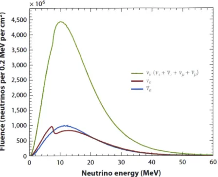
Figure 4-3: Expected supernovae neutrino energy spectrum, separated by flavor. Spectrum is integrated over 10 seconds and is based on the

Gava-Kneller-Volpe-McLaughlin model [24].

The lower the threshold, the more candidate events are available for analysis.

How-ever, there are concerns about using the lower energy neutrinos as they may instead be geoneutrinos or produced by nuclear reactors. The expected spectrum of neutrino energies from a core collapse supernovae is shown in Figure 4-3. We can see that the peak occurs around 10 MeV. For the purposes of this study, we choose 7.5 MeV as our neutrino energy threshold as this includes the majority of the supernova peak but excludes the expected energy range for geoneutrinos and reactor neutrinos [25].

4.4 Chosen KamLAND neutrino events

The KamLAND data chosen for this analysis consists of 65 delayed-coincidence event pairs with energies above 7.5 MeV. These events occurred between unix time 1037021184.0

to unix time 1370349815.0 (11 November 2002 to 4 June 2013). This gives a live time

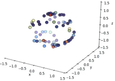
of 3.33 x 108 seconds. The energy distribution of these events is shown in 4-6. The lowest energy event is at 7.53 MeV and the highest is at, 99.37 MeV. The event data includes the location in the detector in which the event occurred; from Figure 4-4, we can see that these events are fairly evenly distributed in the KamLAND fiducial volume.

(30)

Detector locations of prompt events for 7.5 MeV threshold 600 . S S * 400 00 * ₂₀₀ 40 *-600 -800 600 400 200 -800600 0 X 400 60 -600 600 800-800

Figure 4-4: Distribution of > 7.5 MeV neutrino events in the KamLAND detector

volume.

Event energy vs time for 7.5 MeV threshold

x X x x X x x XX x x x x x X x x X 2006 2008 Time of Event x x X x X x x X X 2010 2012

Figure 4-5: Candidate KaniLAND neutrino events (Energy > 7.5 MeV), plotted by

energy and time.

30

I

100 x 80 -60 x

I

5 (U Cj ai X x 40 x 20 -0 x XXx x X XX XX 2004 -x x x

(31)

Event energies for 7.5 MeV Threshold

7.5 17.5 27.5 37.5 47.5 57.5 67.5 77.5 87.5 97.5 107.5

23 3 4 5 6 4 2 8 8 2

35% 5% 6% 8% 9% 6% 3% 12% 12% 3% Neutrino Energy (MeV)

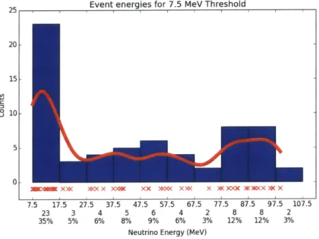
Figure 4-6: Energy distribution of candidate neutrino events above 7.5 MeV threshold. The red curve shows a normalized Gaussian smoothing of the event energies. The red x's below the histogram show the exact energies of the events. Bins were chosen to be 10 MeV wide, starting at the threshold of 7.5 MeV. The standard deviation of the Gaussian is 5 MeV. Counts and percentage of total events that, fall into in a given bin are also labeled. We can see that the majority of the events (35%) are between

7.5 MeV and 17.5 MeV, with the remainder ranging up to 107.5 MeV. The highest

energy event is actually 99.37 MeV.

25 20 15- 10-Ln 0 U 5 0 A

W'mm"

(32)

4.5 LIGO

LIGO consists of two interferometer facilities, one located in Hanford, Washington

and the other located in Livingston, Louisiana. These two locations are separated by about 3002 km 126]. Each LIGO interferometer consists of an L-shaped detect with 4 km long vacuum chamber arms. At the vertex of the L and at the end of each of the arms are hung test masses fitted with mirrors. Laser beams measure the effect of gravitational waves on the test masses. The interferometers are sensitive enough to detect length changes on the order of 10-18 meters, making LIGO capable of detecting gravitational waves between 30 and 7000 Hz [27]. Data collection for initial LIGO occurred between 2002 and 2010, when initial LIGO was upgraded to Enhanced

LIGO. Currently, LIGO has recently completed upgrades to become Advanced LIGO.

Because LIGO is so sensitive to vibrations, it is easy to create a fake signal; even trucks driving on a nearby road can disrupt the detector. The long separation between detectors decreases the chance that environmental noise will occur simultaneously in both detectors and result in a false correlation [26]. The LIGO Scientific Collaboration frequently performs joint analyses with the Virgo Collaboration, which adds an add an additional level of discrimination against fake signals due to the Virgo detector's separation from both LIGO detectors.

4.6 Detecting Gravitational Waves with LIGO

In order to perform a multimessenger search for core-collapse supernovae, a triggered search would be performed on LIGO's data using neutrino events as the triggers. Such a search looks for events over a period of time spanning the approximate ex-pected discrepancy in arrival time between neutrinos and gravitational waves, which is usually between 0 and 20 seconds. We can compare the time stamp of the potential events found to the time stamp of the trigger event and determine how likely it is that a gravitational wave event occurred in the required time frame. This simulated triggered search contains a single event; in a real simulated triggered search, we would

(33)

potentially have multiple possible gravitational wave events to consider.

Once a potential gravitational wave event has been identified, there are two tasks at hand. First, determine if the event is likely to be a real event. Second, determine if it originated from the same source as the trigger event. In order to determine whether or not the event is a real event, we calculate the signal to noise ratio p, which is explained in more detail below [28][29]. Once the event has been determined to be above the threshold to be considered to be a valid event, we look to see if the event could have been caused by the same supernova, or other astronomical event, that initiated the trigger event. The time stamp of the event in three separate detectors allows for triangulation of the event's location.

Ideally, we would then compare this to the triggering event's expected location. (i.e. the location of the supernova). Since we do not have a way of independently determining the location of the supernova, the best we are able to do is to compare the location of the probable event to the galactic disk's location. The event is much more likely to occur in the plane of the galactic disk because of the greatly increased number of stars and thus potential supernova candidates.

If possible, the location implied by the gravitational waves could then be compared

to the direction from which corresponding neutrino events originated. This would require a directional neutrino detector. The KamLAND data does not provide any directionality information, but a water Cerenkov detector like Super-Kamiokande, or a future directional liquid scintillator experiment would provide an extra way to check that the events come from the same location [30]. Better photodetectors with more complete photocathode coverage and improved timing resolution can assist in directional sensitivity, as can the choice of scintillators which enhance the ability to discriminate between the Cereknov light and isotropic scintillation light [30].

4.7 Noise-discrimination in Gravitational Wave Events

One of the biggest difficulties in detecting gravitational waves is extracting the grav-itational wave signal from the noise. Gravgrav-itational wave signals are exceptionally

(34)

weak, and the noise background is quite complicated. Because of the non-Gaussian and non-stationary nature of the background noise, it cannot be accurately modeled and instead is accounted for via a time shift. By determining how much the data must be shifted in time in order to find a correlated signal at another detector, it can be determined whether or not the signal is a real event or is a background signature

[31].

In order to address the non-Gaussian non-stationary noise, real data is used to make an estimated background. There is no way to shield the detector from gravi-tational waves and produce an eventless signal, but this challenge can be overcome using multiple data streams from separate detectors [31]. The data from one detector is time-shifted by some chosen step size and then recombined with the data from another detector. The step size is chosen to be much longer than the time of flight

between detectors (- 30 ms) and the coherence time scale of the detector noise (a few

seconds)

[31].

This scrambles any actual gravitational wave signals. By repeating the shifting procedure hundreds of times, each with a different relative time shift among detectors, we can obtain an accurate estimate of the rate of background events. Once the time shift and recombination has occurred, the only remaining "events" would be caused by coincidences in instrumental glitches [31]. Data quality studies are used to flag background events which might correspond to instrumental and data acqui-sition artifacts, periods of degraded sensitivity, or excessive transient environmental noise [17]. The significance of a gravitational wave event can then be computed by determining the fraction of background events which are louder than the prospective gravitational wave events [31].

The gravitational wave signals can be characterized in several ways, two of which are the event's amplitude, h,,,, and signal to noise ratio, p [32]. Because gravitational waves interact so weakly with matter, they are largely unaffected by their passage through matter and are not absorbed or scattered. This allows them to cleanly carry information between the source and the observer [33]. The signal-to-noise ratio and the amplitude thus have a simple scaling; they scale inversely with luminosity distance, which leads to a universal signal-to-noise distribution of gravitational wave

(35)

events, where the number of valid events is based only on the distance from the source and the chosen SNR threshold. This assumes that the source population does not evolve with distance, which is valid in our case because LIGO only has sufficient sensitivity to probe the nearby universe, with redshift z < 0.2 [33].

The sensitivity of LIGO depends on the desired threshold for signal to noise ratio,

p, that is demanded of the gravitational wave candidates. In general, for a signal

h(t),4

df 12

1/2

JO SWf

where h(f) is the Fourier transform of h(t), and S(f) is the one-sided power spectral density of the detector noise [32]. Traditionally, S(f) assumes that the noise is Gaus-sian, which is not the case for LIGO [32]. To account for the non-Gaussian nature of the noise, the time-shift analysis is used to generate a sample background for use in computing p

[341.

The detectability of a given gravitational wave signal is charac-terized by the gravitational wave amplitude, which is given by the root-sum-square strain amplitude, hrs, defined as [17]:

hrss = |h+(t)|2 _{+ hx(t)}2_dt

where h+(t) and hx (t) are the dimensionless amplitude components for each of the two independent signal polarizations. The detector response, meanwhile, is given by the linear mixture of the two polarization components

hdet(t) = F+h+(t) + Fx hx (t)

where F+, Fx are the antenna pattern factors, which are characterized by the way the different wave polarizations coupled to the detector [31]. In a multimessenger study, the hrs, and p values would be used in determining the likelihood that an candidate event is a true gravitational wave event.

(36)

(37)

Chapter 5 Results

5.1 Neutrino-only correlation search

I did a search of the set of neutrino data alone to determine if any correlations

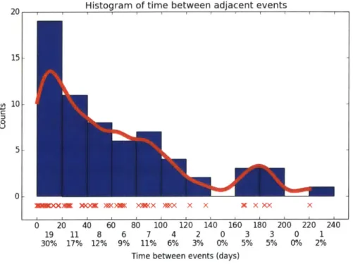
be-tween events were present. The method was modeled from KamLAND's earlier study, which uses a slightly different data set. The time distribution of the 65 candidate neutrino events over 7.5 MeV is shown in Figure 4-5. Examining the time delay be-tween subsequent events, we find no delayed coincidence event-pairs of events within a 20 second coincidence window, except for one pair of anomalous events which will be discussed momentarily. The shortest delay between subsequent events is 74686 seconds, or about 20.7 hours. Only one pair of events occurred in the same 24 hour period. The longest delay between subsequent events is 220 days. The distribution of time gaps between subsequent events is shown in Figure 5-1. Since the neutrino data alone reveals no bursts which might be attributed to a supernovae, we need the improved sensitivity of a multimessenger study to search for core-collapse supernovae with KamLAND.

The pair of anomalous events is a pair of prompt events with identical time stamps. The two prompt events both appear to correspond to the same delayed event. This may have been a fast neutron event caused by a muon moving through rock or the outer detector and triggering the two high energy scatterings; however only one of the subsequent captures was also detected.

(38)

20 15 0 U 10 5 0

Histogram of time between adjacent events

0 20 40 60 80 100 120 140 160 180 200 220 240

19 11 8 6 7 4 2 0 3 3 0 1 30% 17% 12% 9% 11% 6% 3% 0% 5% 5% 0% 2%

Time between events (days)

Figure 5-1: Time between subsequent KamLAND neutrino events with energy above

7.5 MeV. The red curve shows the normalized Gaussian smoothing of the time gaps.

The standard deviation of the Gaussian is 10 days, chosen to be half the bin width

of 20 days. The red x's show the actual time gaps between events.

(39)

Fx/nt energy vs time for 7.5 MeV threshold. GW event marked by line 80- x x -x K X 60 - K X x K K K LU C 40- X LU X 20 x X -K K 0 1.00 1.05 1.10 1.15 1.20 1.25 1.30 1.35 1.40

Time (unix) le9

Figure 5-2: Timle and energy of the candidate neutrino events. The sample gravita-tional wave event is marked with a line. The closest neutrino event occurs 14.03 days

after the gravitational wave event.

5.2 Analysis of sample gravitational wave event

Because there is no data sharing agreement between LIGO and KamLAND, this analysis was done using a single sample event, and could be easily expanded if more data was available. Our single LIGO candidate gravitational wave event data file was produced in the same manner as data that would have been produced by a triggered search using KanLAND neutrinos as triggers.

Because this is sample data and is not triggered by a neutrino event, unsurpris-ingly, it does not happen to be close in time to any of the neutrino events. This sample

event occurred at unix time 1287490320.31 (October 19, 2010, at 12:12 UTC). There

is a neutrino event above the 7.5 MeV threshold detected by KamLAND at unix time

1288703129 (November 2, 2010 at 13:05 UTC). The next-closest event occurred at

unix time 1282946808 (Aug 27, 2010 at 22:06 UTC). This is shown in relation to the time of the candidate neutrino events in Figure 5-2. In this case we did not expect to find any time correlation between the gravitational wave event and the neutrino

x x

X X X

(40)

Potential source locations of GW events. Red: highest probability 1.5 1.0 0.5 4 . 0.0 z b -0.5 Cqc- -"-1.0 0~ - 1.5 1.5 1.0 0.5 -1.5 _1.0 _0.0 -5 _0.0 _0.1-00.5 1.0 1.5 -1.5

Figure 5-3: Possible trigger event locations, with the higher probability locations denoted by redder colors and the lowest probability locations denoted by the purple colors. The highest, probability pixel, denoted by the red point, has a probability of

6.69 x 10-2. The lowest, probability pixel, denoted by purple, has a probability of 6.91 x 10-4. The probabilities of each location sum to one.

events; however, in a real search finding a time correlation would be the vital first step.

After determining if the events are appropriately time-correlated, we would con-sider carefully the values of p and hrss corresponding to the event. For the sample event, p = 59.71. Whether this is above the threshold to be determined a real event would depend on the parameters of the study. The triggered event, also contains the

signal-to-noise ratio and It, for each of three available detectors. (For example, hr,

is 4.69 x 10-21, 3.29 x 10-21, and 3.40 x 10-21, respectively.) The frequency of the

potential gravitational wave characterized by this event is 396.58 Hz.

The time of the sample event in each detector is (in GPS time), 971525503.3060,

971525503.3057 and 971525503.3045 respectively. There is a delay of between 0.3 ns

and 1.5 ins between detectors, which allows for triangulation of the event's location. The file includes the right ascension and declination of the possible event locations

(41)

and the probability that the event occurred in that pixel of sky. We can use this to determine the likely source location of the event. The scatter plot in Figure 5-3 shows the likely location of the sample event in the sky, plotted using the spherical coordinates given in the sample event file.

In Figure 5-3, we have recolored the points according to the probability that the event occurred in that location. We can see that the event most likely came from a source directly above the detector. The subsequent step in an actual multimessenger search would be determining whether or not this event falls within the galactic plane and, if possible, whether the corresponding neutrino event came from the same direc-tion. This would then be repeated for all candidate gravitational wave and neutrino events.

5.3 Joint false alarm rate

The joint false alarm rate, Rj, is given by:

R3 = RGW x R, x w

where RGW is the gravitational wave background rate, R, is the neutrino background rate, and w is the coincidence window.

The KamLAND data spans 3.33 x 108 seconds. There are 65 events over the chosen 7.5 MeV threshold. This gives a background rate of:

65 events

R= - 65 s - 1.95 x 10-7 Hz

3.33 x 108 sec

We make the following approximation of the all-sky gravitational wave search false-alarm rate

135]:

(42)

and we choose coincidence windows of w = 2 sec and w = 20 sec, we find: R1 (2 s) = 3.5 x 10-9 - 1.95 x 10-7 .2 = 1.37 x 10-15 Hz

Rj(20 s) = 3.5 x 10-g - 1.95 x 10-7 .2 = 1.37 x 10-14 Hz

The 20 second coincidence window corresponds to a false alarm rate of 1 event per 2.32 x 106 years.

(43)

Chapter 6 Conclusion

In summary, a joint neutrino and gravitational wave search for core-collapse super-novae provides a much better look at core-collapse supersuper-novae than either neutrinos or gravitational waves can provide alone. Since neutrinos and gravitational waves carry different kinds of information about their source supernovae, a multimessenger search is not only more accurate, but also more informative.

Both LIGO and KamLAND are highly sensitive detectors, but to date no super-novae signatures have been reported by either collaboration. Collaborations between LIGO and other neutrino experiments, such as ANTARES and IceCube, have al-ready yielded valuable results and useful limits on source prevalence. Both IceCube and ANTARES, however, are primarily sensitive to GeV neutrinos and higher; only KamLAND is sensitive in the ~ 10 MeV region where supernovae neutrinos are ex-pected to reside. This makes KamLAND a better detector to do a multimessenger search of this form.

By leveraging the low backgrounds of both LIGO and KamLAND, a much lower

false-alarm rate can be achieved, leading to a more accurate limit on the source den-sity of core collapse supernovae and, potentially, detection of supernovae. Through a collaboration between these two top-of-the-line detectors, we can glean new infor-mation about core collapse supernovae, and further our understanding of this vital astrophysical phenomena.

(44)

(45)

Bibliography

[1] KamLAND Collaboration, K. Eguchi et al., Phys. Rev. Lett. 90, 021802 (2003). [21 T. Foglizzo et al., Publications of the Astronomical Society of Australia 32

(2015).

131

Australia Telescope National Facility, Post-Main Sequence Stars, http://www.atnf.csiro.au/outreach//education/senior/astrophysics/ stellarevolution-postmain.html, Accessed: 2015-11-25.

[4] Australia Telescope National Facility, The Death of Stars I:

Solar-Mass Stars, http://www.atnf.csiro.au/outreach//education/senior/

astrophysics/stellarevolution-deathlow.html, Accessed: 2015-11-25.

[5] K. Kotake, K. Sato, and K. Takahashi, Reports on Progress in Physics 69, 971 (2006).

[6] S. Woosley and T. Janka, Nat Phys 1, 147 (2005). [7] J. W. Murphy and J. C. Dolence, (2015), 1507.08314.

[8] K. Belczynski, G. Wiktorowicz, C. L. Fryer, D. E. Holz, and V. Kalogera, The

Astrophysical Journal 757, 91 (2012).

[9] Australia Telescope National Facility, The Death of Stars II: High

Mass Stars, http://www.atnf.csiro.au/outreach//education/senior/

astrophysics/stellarevolution-deathhigh.html, Accessed: 2015-11-25.

[10] S. Ando, J. F. Beacom, and H. Yiiksel, Phys. Rev. Lett. 95, 171101 (2005).

[11] ANTARES Collaboration and LIGO Scientific Collaboration and Virgo

Collab-oration, Journal of Cosmology and Astroparticle Physics 2013, 008 (2013). [12] P. Blasi, Particle acceleration, http://fermi.gsf c.nasa.gov/science/mtgs/

summerschool/2012/week1/CR2 _Blasi.pdf, Accessed: 2016-01-02.

[13] K. D. Kokkotas, Gravitational Wave Astronomy (Wiley-VCH Verlag GmbH &

Co. KGaA, 2008), pp. 140-166.

(46)

[15] LIGO Scientific Collaboration and Virgo Collaboration, Phys. Rev. D 81, 102001

(2010).

116] GEO600 technical principles, http://www.geo600.org/1077324/Technical

Principles, Accessed: 2015-12-24.

1171

LIGO Scientific Collaboration and Virgo Collaboration, Phys. Rev. D 85,122007

(2012).

[18] D. Guetta, T. Piran, and E. Waxman, Astrophys. J. 619, 412 (2005), astro-ph/0311488.

[191 IceCube Collaboration and LIGO Scientific Collaboration and Virgo

Collabora-tion, Phys. Rev. D 90, 102002 (2014), ArXiv: 1407.1042.

[20] KamLAND Collaboration, K. Asakura et al., The Astrophysical Journal 806,

87 (2015).

[21] KamLAND physics impact, http://kamland.lbl.gov/PhysicsImpact/, Ac-cessed: 2015-12-25.

[22] KamLAND Collaboration, S. Abe et al., Phys. Rev. C81, 025807 (2010),

0907.0066.

[23] K. Asakura et al., (2015), 1506.01175.

[24] K. Scholberg, Ann. Rev. Nucl. Part. Sci. 62, 81 (2012), 1205.6003.

[25] KamLAND Collaboration, A. Gando et al., Phys. Rev. D88, 033001 (2013), 1303.4667.

[26] LIGO facilities, https://ligo.caltech.edu/page/facilities, Accessed:

2015-12-20.

[27] LIGO fact sheet, http://labcit.ligo.caltech.edu/LIGO-web/about/

fact sheet .html, 2001, Accessed: 2015-12-20.

[281 E. Thrane and J. D. Romano, Phys. Rev. D 88, 124032 (2013).

[29] A. Lazzarin, The analysis of LIGO data, http: //elmer. tapir. caltech. edu/

ph237/week15/GO20222-0O.pdf, LIGO-G20222-00-E.

[30] L. Winslow, Next-Generation Liquid-Scintillator-Based Detectors: Quantums

Dots and Picosecond Timing, in Community Summer Study 2013: Snowmass on the Mississippi (CSS2013) Minneapolis, MN, USA, July 29-August 6, 2013,

2013, 1307.2929.

[31] LIGO Scientific Collaboration and Virgo Collaboration, E. Chassande-Mottin,

(47)

[32] P. Sutton, The Signal-to-Noise Ratio as a Predictor of Detectability in the S1

Burst Search, 2004, LIGO-T040002-00-Z.

[33] H.-Y. Chen and D. E. Holz, (2014), 1409.0522.

[34] S. Klimenko and C. Pankow, Detection statistic for multiple algorithms, net-works, and data sets., 2012, LIGO-T-1200169.

[35] Neutrinos meet gravitational waves: Preparing for the next nearby core-collapse

supernova, 2013.

[36] C. L. Fryer, D. E. Holz, and S. A. Hughes, The Astrophysical Journal 565, 430

(2002).

[37] B. S. Sathyaprakash, Gravitational radiation: Observing the dark and dense

uni-verse, in Proceedings, 28th International Cosmic Ray Conference (ICRC 2003),

pp. 49-74, 2004, gr-qc/0405136.

[38] U. Keshet and S. Balberg, Phys. Rev. Lett. 108, 251101 (2012).

[39] C. Aberle, A. Elagin, H. J. Frisch, M. Wetstein, and L. Winslow, JINST 9, P06012 (2014), 1307.5813.

[40] Super-Kamiokande Collaboration, The Astrophysical Journal 669, 519 (2007). [41] E. Waxman and J. Bahcall, Phys. Rev. Lett. 78, 2292 (1997).

[42] K. L. Dooley, T. Akutsu, S. Dwyer, and P. Puppo, Journal of Physics: Conference Series 610, 012012 (2015).

Detection of core-collapse supernovae through joint analysis of LIGO gravitational wave and KamLAND neutrino data