Open Archive TOULOUSE Archive Ouverte (OATAO)
OATAO is an open access repository that collects the work of Toulouse researchers and
makes it freely available over the web where possible.
This is an author-deposited version published in:
http://oatao.univ-toulouse.fr/
Eprints ID : 14633
To link to this article : DOI :10.1016/j.cma.2015.11.007
URL :
http://dx.doi.org/10.1016/j.cma.2015.11.007
To cite this version: Bouclier, Robin and Passieux, Jean-Charles and
Salaün, Michel
Local enrichment of NURBS patches using a
non-intrusive coupling strategy: Geometric details, local refinement,
inclusion, fracture.
(2016)
Computer Methods in Applied Mechanics and Engineering, vol.
300. pp.1-26. ISSN 0045-7825
Any correspondance concerning this service should be sent to the repository
administrator:
[email protected]
Local enrichment of NURBS patches using a non-intrusive coupling
strategy: Geometric details, local refinement, inclusion, fracture
Robin Bouclier
a,∗, Jean-Charles Passieux
b, Michel Sala¨un
baUniversit´e de Toulouse, Institut de Math´ematiques de Toulouse, UMR CNRS 5215, INSA-Toulouse, 135 avenue de Rangueil, F-31077 Toulouse Cedex 04, France
bUniversit´e de Toulouse, Institut Cl´ement Ader, FRE CNRS 3687 INSA/UPS/ISAE/Mines Albi, 3 rue Caroline Aigle, 31400 Toulouse, France
Highlights
• We address the issue of modelling local phenomena in a NURBS patch with a global/local non-intrusive algorithm. • The approach provides simplicity and flexibility to treat any case of local enrichment in a NURBS patch.
• We propose a strategy to handle non-conforming geometries.
• We demonstrate the performance of the method on a range of two-dimensional linear elastic numerical examples.
Abstract
In this work, we apply a non-intrusive global/local coupling strategy for the modelling of local phenomena in a NURBS patch. The idea is to consider the NURBS patch to be enriched as the global model. This results in a simple, flexible strategy: first, the global NURBS patch remains unchanged, which completely eliminates the need for costly re-parametrization procedures (even if the local domain is expected to evolve); then, easy merging of a linear NURBS code with any other existing robust codes suitable for the modelling of complex local behaviour is possible. The price to pay is the number of iterations of the non-intrusive solver but we show that this can be strongly reduced by means of acceleration techniques. The main development for NURBS is to be able to handle non-conforming geometries. Only slight changes in the implementation process, including the setting up of suitable quadrature rules for the evaluation of the interface reaction forces, are made in response to this issue. A range of numerical examples in two-dimensional linear elasticity are given to demonstrate the performance of the proposed methodology and its significant potential to treat any case of local enrichment in a NURBS patch simply.
Keywords:Isogeometric analysis; NURBS; Non-intrusive coupling; Domain decomposition; Non-conforming geometries; Fictitious domain approach
∗Corresponding author.
E-mail addresses:[email protected](R. Bouclier),[email protected](J.-C. Passieux),[email protected]
replaced by Non-Uniform-Rational-B-Spline (NURBS) functions to perform the analysis. NURBS functions have a higher order of continuity, namely C(p−1) through the knot-span elements of the mesh for a polynomial degree p, which, on a per-degree-of-freedom basis, gives increased accuracy in comparison with standard Finite Element Methods (FEM) (see, e.g., [3] for a theoretical analysis, [4] for applications in structural vibrations, [5] for problems of standard elasticity, [6] for embedded domain methods and [7,8] for shell analysis). Although the global accuracy of NURBS is now proved, the rigid tensor product structure of these functions still prevents simple modelling of local behaviours in a NURBS patch. For example, the integration of geometric details (i.e., basically, holes) leads to the analysis of a trimmed NURBS patch, which is not a trivial task. The basic strategy may involve a re-parametrization of the NURBS model, including the splitting of the new geometry into several patches with C0 continuity at the boundaries. This may apply not only for geometric details but to all situations of local models different from the global NURBS patch model (e.g., local refinement, inclusion [9], local fracture [10,11], local plasticity [12], etc.). This entails a considerable modelling effort that is often as complex and time consuming as standard mesh generation and so is opposed to the core idea of IGA, which advocates a direct link between geometry and analysis.
After the pioneering works on NURBS-based IGA, great interest in methods addressing these modelling questions has emerged in the field. One of the most noteworthy is the development of new splines that enable local refinement: hierarchical B-splines and NURBS [13,14], LRB-splines [15], T-splines [16,17] and multigrid-based NURBS [18]. Among these strategies, T-splines seem to have gathered considerable momentum in both the computational geometry and analysis communities since they also appear suitable to address trimmed multi-patch geometries. Nevertheless, the implementation of these new IGA techniques can appear complex and additional efforts may be necessary to solve the issue of describing a local behaviour that is different from the global behaviour (inclusion, local fracture, local plasticity).
Concurrently, a second recent approach initiated in Nguyen et al. [9] and Ruess et al. [19] and based on the combination of the Finite Cell Method (FCM) with Nitsche coupling may constitute an interesting option to resolve our problem of modelling local behaviours in a NURBS patch. The FCM, which combines the fictitious domain approach with higher-order finite elements and adaptive integration, has proved to be efficient for the analysis of any arbitrary trimmed patches (see, e.g., [20] for a detailed review). Regarding NURBS coupling, a great effort has been made concerning the connection of NURBS patches in recent years. One of the first works on the subject was certainly that of Hesch and Betsch [21], who used the Lagrange multiplier method to couple NURBS solids. Then, a comparative study in Apostolatos et al. [22] showed the efficiency of a Nitsche-based technique for NURBS. In consequence, Nitsche coupling has been used for connecting 3D NURBS patches [9], for 3D-plate NURBS coupling [23,24], and with NURBS immersed boundary methods [25,19]. Although it appears interesting because of the strong mathematics behind it and the absence of additional degrees of freedom, the Nitsche method leads to considerable implementation work and an increased cost of computation, since an additional eigenvalue problem has to be solved for the stabilizing term. As a result, Dornisch et al. [26] has recently developed a weak substitution method that can be interpreted as a mortar method. Although the combination of the FCM with Nitsche coupling may be promising, the drawback of such a strategy, if directly applied to the local enrichment of a NURBS patch, is that it suffers from some intrusiveness. More precisely, two main limitations can be highlighted. On the one hand, the introduction of a local zone within the NURBS patch requires a re-parametrization of the global geometric model, which is not a trivial task in the NURBS framework. This can be very time consuming, in particular when the local region is expected to evolve (e.g., shape optimization of the geometric details, of the inclusions, crack propagation, expansion of the plastic zone) since several re-constructions and re-computations of the whole problem then have to be performed during the simulation. On the other hand, it is to be noted that, when Nitsche-based methods are used, both the global and local operators have to be modified and merged together for the coupling, which implies significant implementation efforts and a monolithic resolution and thus prevents the simple use of existing robust codes for the global/local strategy.
To overcome this difficulty, the alternative purpose of this work is to make use of a non-intrusive global/local coupling strategy that has become popular in FEM. Based on the idea of Whitcomb [27], formalized later by Gendre
et al. [12], for the modelling of local plasticity, the method that we consider in this work involves the definition of two finite element models: a global, coarse model of the whole structure and a local, more detailed “sub-model” meant to replace the global model in the area of interest. An iterative coupling technique is used to perform the substitution in an exact but non-intrusive way: only interface data are transmitted from one model to the other and the global stiffness operator remains unchanged (independently of the shape of the local domain). This strategy has been applied in FEM for the modelling of crack propagation [11], for the modelling of localized uncertainties [28], for 3D-plate coupling [29] and for nonlinear domain decomposition [30]. Let us note that this methodology, involving the coupling of a global model and a local model in an iterative manner, has similarities with some hierarchical global/local methods in FEM: for example, the Chimera method [31], the method of finite element patches [32], numerical zoom [33] or the hp − dmethod [34–36]. However, the difference of the strategy considered here is that the contribution of the global solution in the local area is totally replaced by the local solution while, in the hierarchical strategy, an approximate solution is sought as the sum of the global coarse contribution and a local fine one. As a result, the advantage of the algorithm used is that it reduces the interactions between global and local discretizations. In the proposed approach, the two models talk to each other with interface integrals only, while the evaluation of mixed terms over the whole local domain is necessary in the hierarchical approach. In this sense, the strategy followed in this work is said to be non-intrusive.
In this paper, we propose an application of the non-intrusive technique [27,12,11,28–30] to the NURBS context. The idea is to take the NURBS patch to be enriched as the global model. In consequence, the global patch is never modified during the simulation, which eliminates the need for costly NURBS re-parametrization procedures. In addition, the global stiffness operator is assembled and factorized only once and the system to be solved remains well-conditioned. If the local behaviour is expected to evolve, only the local model (including a limited number of degrees of freedom since restricted to a thin zone of the structure) has to be re-computed. Moreover, it should be mentioned that the flexibility of the strategy allows simple modelling of a variety of local behaviours. Since the global and local problems are solved alternately in a non-intrusive strategy, two different numerical codes can be used to compute the global and local models. Thus, a linear NURBS code can be used for the global modelling of the NURBS patch while any other existing robust code integrating any other numerical method can be used to incorporate an accurate local model. By making use of this strategy, we are able to address geometric details (for which the local model is void: it represents holes) as well as all other cases of local models that are covered: e.g., refined mesh, inclusion, fracture, plasticity. In particular, we successfully apply the non-intrusive approach in this work for the situation of holes, local refinement, inclusion and local fracture in a two-dimensional NURBS patch under linear elasticity.
The difficulty when applying the non-intrusive strategy to NURBS is that non-conforming geometries need to be addressed. By non-conforming geometries, we mean that the local model domain overlaps the knot-span elements in the global NURBS patch as the local model domain may be bounded by a trimming curve living in the interior of the global NURBS patch to be enriched. Thus, given the rigid tensor product structure of the NURBS, there is no reason for the boundary of the local model domain to be aligned with the edges of the global NURBS patch elements. The non-conforming geometries issue does not involve specific modifications of the equations and associated weak forms but special attention is needed in the implementation process. In particular, the evaluation of the reaction forces of the complement part of the global model (the part meant to be replaced in the non-intrusive algorithm) requires the setting up of a suitable quadrature rule and its treatment in the global NURBS patch. For this purpose, an exact NURBS domain is simply constructed from the NURBS trimming curve in the case of a geometric detail while the quadrature rule used for the local model is transposed within the global NURBS patch in the case of real (covered) local models. With regard to coupling, an application of the conventional Lagrange multiplier approach to non-conforming geometries is employed to meet the non-intrusive constraint in the sense of [11,29,30]. Acceleration techniques, such as techniques based on Aitken’s Delta Squared method or a Quasi-Newton method (see, e.g., [30]), are also implemented in the present situation, which results in a significant reduction of the number of iterations of the non-intrusive algorithm.
The paper is organized as follows: after this introduction, Section2reviews the fundamentals of NURBS-based IGA and introduces the reference global/local coupling problem to be solved. Then, Section3 is devoted to the application of the non-intrusive global/local strategy to the NURBS context. In particular, the study is divided into two parts: the situation of geometric details involving a void local model is investigated before the more usual case of covered local models is addressed. Section4presents a range of numerical examples in two-dimensional linear elasticity that demonstrate the performance of our methodology and its significant potential for the simple treatment
This section establishes the context of the study and introduces the corresponding notations. We start with a brief review of the concept of NURBS-based IGA with a particular emphasis on the trimming concept that may facilitate the geometric modelling of local behaviours. Then, the reference global/local problem is presented along with its standard weak coupling formulation.
2.1. Nurbs-based isogeometric analysis 2.1.1. Basics
For the discretization, we will use the recent concept of IGA based on NURBS functions. Only the fundamentals of the concept are given in the following. For further details, the interested reader is referred to the references cited below.
The NURBS concept was first introduced in Hughes et al. [1] and formalized more recently in the book by Cottrell et al. [2]. NURBS functions are a generalized version of B-spline functions and have become a standard for geometric modelling in CAD and computer graphics (see, for example, Cohen et al. [37], Piegl and Tiller [38], Farin [39] and Rogers [40]). These functions lend themselves to an exact representation of many shapes used in engineering, such as conical sections. They can be viewed as rational projections of higher-order B-splines and, therefore, they possess many of the properties of B-splines, the most interesting one being their high degree of continuity.
For the presentation in this part, we consider a domain in 3D so as to be general. If (NA)A∈{1,2,...,n} denote the
n 3D NURBS functions,(ωA)A∈{1,2,...,n}the associated weights and(PA)A∈{1,2,...,n}the associated control points of
coordinates(xA)A∈{1,2,...,n} in the global coordinate system, the geometry of the structure is described through the
position vector M defined as:
M =
n
A=1
NAxA, (1)
where the NURBS functions are obtained from the B-spline functions NA
A∈{1,2,...,n}such that:
NA= NAwA n A=1 NAwA . (2)
Now, all one needs to do in order to define the 3D B-spline functions NA at control point PA is to perform the
tensor product of the 1D B-spline functions associated with this point in the three spatial directions. If one denotes M1 i i ∈{1,2,...,n1}, M2j j ∈{1,2,...,n2} and Mk3k∈{1,2,...,n
3}the n1, n2and n31D B-spline functions associated with each
of the three spatial directions, this means that at control point PA, which corresponds to the i th, j th and kth control
points in these directions, one has: NA=Mi1×M
2 j ×M
3
k. (3)
The 1D B-spline functions are defined using a knot vector. Each knot vector associated with a direction is defined in the parametric domain. For example, for the first direction, one takes knot vector Ξ =ξ1, ξ2, . . . , ξn1+p+1, where
ξl ∈ R is the lth knot, with l being the knot index (l = 1, 2, . . . , n1+ p +1) and p the polynomial degree of
the functions Mi1i ∈{1,2,...,n
1}. The knots divide the parametric space into elements, and the interval
ξ1, ξn1+p+1
constitutes the IGA patch. The patch may be thought of as a macro-element. Most geometries utilized for academic test cases can be modelled with a single patch. In two-dimensional topologies, a patch is a rectangle in the parametric domain. In three dimensions it is a cuboid.
Remark 1. In this work, we need to be careful with the term “patch” since this one can be employed for both NURBS and global/local coupling algorithm. We emphasize here that the term “patch” will only refer to the concept of IGA patch in the following. Thus, the term patch will never refer to the local model (in opposition to [32] for example).
Unlike standard FEM where each element has its own parametrization, the parametric space of B-Spline functions is localized onto the patch. There can be more than one knot at a given location of the parametric space. If m is the multiplicity of the considered knot, the functions have Cp−mcontinuity at that location. If the knots are evenly spaced,
the knot vector is said to be uniform. A knot vector whose first and last knots have multiplicity p + 1 is said to be open. In this case, the basis is interpolating at the boundary knots of the interval, which facilitates the application of the boundary conditions. For the sake of simplicity, we will consider in this work geometries that can be represented (excluding the local details) with the use of only one patch. Furthermore only open uniform knot vectors will be considered. The 1D B-spline basis functions for a given order p are defined recursively from the knot vector using the Cox–de Boor recursion formula (see, for example, Cohen et al. [37]).
To take advantage of the superior approximation properties of NURBS functions, one chooses them to be at least of polynomial degree two in all the spatial directions. As far as continuity is concerned, one performs k-refinement, meaning that one adds elements while keeping the higher degree of continuity of the NURBS functions, namely Cp−1 at the knot level. The positions of the control points and the values of the associated weights can be adjusted in order to build conical sections exactly, after which these geometries are preserved through mesh refinement. For a good overview of mesh generation and refinement, see Cottrell et al. [41].
2.1.2. The trimming concept
The difficulty to model local behaviours in a NURBS patch is due to the use of the tensor product (see Eq.(3)). For example, this makes the integration of geometric details (e.g., holes) in a NURBS patch far from trivial. Indeed, since standard IGA technology requires a boundary fitted discretization for the analysis, a re-parametrization of the whole NURBS model taking into account the geometric detail is required. This may lead to the splitting of the new geometry into several patches with C0continuity at the boundaries. This entails a considerable modelling effort, which is often as complex and time consuming as standard mesh generation as explained in [19]. In CAD programs, where the only need is the rendering of the geometry, such a re-parametrization is not necessary. Designers make use of the trimming concept to create an almost unlimited range of geometric shapes. The trimming concept is illustrated in 2D for the situation of a circular hole as the geometric detail of a rectangular structure, seeFig. 1. This surface can be classified as a trimmed surface. Its description is simply given by: a one-patch B-Spline surface parametrization for the plate (without the hole) and a NURBS curve parametrization for the trimming curve that forms the boundary of the hole. The trimming curve specifies visible and invisible regions on the surface patch. As a consequence, the underlying NURBS patch remains unaffected by the trimming object and preserves its topology. Conversely, the NURBS parametrization of the plate including the hole (without trimming) is shown inFig. 1(c). As can been seen, a NURBS re-parametrization of the geometry (including the splitting into 4 elements with C0 continuity on the boundary) is necessary.
2.2. Definition of the global/local problem 2.2.1. Governing equations
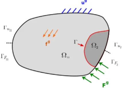
We undertake to study a multi-domain model characterized by a physical domain Ω ∈ Rd, d = 2 or 3, which is divided into two disjoint, open and bounded subsets Ω11and Ω2such that Ω = Ω11∪Ω2and Ω11∩Ω2= ∅. Those
two non-overlapping subdomains share a common interface denoted Γ (seeFig. 2).
Remark 2. As subdomains are open, one would need to write Ω = Ω11∪Ω2to be rigorous. In the paper, we decide
to omit this notation in order to ease the reading.
We suppose that the local part of the problem is the small region Ω2 and that a simple linear elastic model is
sufficient to describe the global behaviour in the complement domain Ω11. Even if the method applies in more general
context, we assume in this work a linear elastic constitutive law in Ω2 as well. We emphasize that Ω2 may also
constitute a geometric detail (i.e., basically, a hole). To obtain this situation, one simply needs to take the Hooke tensor in region Ω2equal to zero. Regarding the NURBS discretization of the problem, domain Ω may constitute a
(a) NURBS parametrization of the trimmed geometry.
(b) CAD rendering.
(c) NURBS re-parametrization (without trimming).
Fig. 1. Illustration of the trimming concept. (For interpretation of the references to colour in this figure legend, the reader is referred to the web version of this article.)
Fig. 2. The reference global/local problem.
NURBS patch and Γ (and so the extension to∂Ω2) may be viewed as a trimming curve that enables to specify the
local part Ω2. Domains Ω11and Ω2are subjected to body forces fg11and fg2, respectively. Furthermore, surface forces
Fg11 and Fg2are associated to boundaries ΓF11and ΓF2 and, displacements u
g 11 and u
g
2are prescribed over boundaries
Γu11and Γu2. The boundaries satisfy the following relations :
ΓFm∪Γum ∪Γ =∂Ωm ΓFm∩Γum = ∅ ΓFm∩Γ = ∅ Γum∩Γ = ∅ with m = 11 and 2.
Remark 3. We emphasize that we restrict ourselves to a domain Ω that can be represented using a single NURBS patch for simplicity in the presentation only. Obviously, the strategy developed in this work straightforwardly applies for the more general case of a multi-patch geometric model.
The problem to be solved is a classical multi-domain linear elastic problem in Ω11 ∪Ω2. In each subdomain,
the kinematic constraints, the equilibrium equations and the constitutive relations have to be verified. Using the subscript m to denote a quantity that is valid over region Ωm, with m = 11 and 2, the corresponding governing
equations read: um=ugm over Γum; div(σm) + fgm=0 in Ωm; σmnm=F g m over ΓFm; σm=Cmε (um) in Ωm. (4)
For the sake of readability, we decided to use bold symbols for first-order tensors while we underline twice the second-and four times the fourth-order tensors. In the above equations,ε (um) denotes the infinitesimal strain tensors, σmthe
Cauchy stress tensors and Cm the Hooke tensors. n11 and n2 represent the outward unit normals to Ω11 and Ω2,
respectively. To complete the formulation of the boundary value problem, the following coupling conditions have to be added:
u11−u2=0 on Γ ;
σ11n11+σ2n2=0 on Γ. (5)
They ensure kinematic compatibility between the coupled domains and equilibrium of the tractions along the coupling interface Γ , respectively.
2.2.2. Weak form
The starting point in the derivation of a non-intrusive strategy in the sense of [11,29,30] is to weakly formulate the coupling problem(4)–(5) with a Lagrange multiplier approach. The development of the non-intrusive coupling formulation is not the subject of this section. Nevertheless, since it is based on the use of a Lagrange multiplier approach, the corresponding classical weak coupling formulation is given here. A standard fixed point solver is also presented to account for the possibility to dissociate Ω11and Ω2in the resolution. These developments constitute the
reference formulation and the standard global/local solver of our coupling problem.
We start by defining the functional spaces Um and Vm over domain Ωm that will contain the solution and trial
functions respectively: Um= um∈ H1(Ωm) d , um|Γum =u g m ; Vm = vm∈ H1(Ωm) d , vm|Γum =0 . (6)
We also introduce M ⊂ L2(Γ )dthe space for the Lagrange multiplier. The formulation involves the set up of the following Lagrangian: L((u11, u2), λ) = 1 2a11(u11, u11) + 1 2a2(u2, u2) − l11(u11) − l2(u2) + b (λ, u11−u2) , (7) where bilinear form amand linear form lmassociated to domain Ωmread:
am(um, vm) = Ωm ε (vm) : Cmε (um) dΩm; lm(vm) = Ωm vm·fgmdΩm+ ΓFm vm·FgmdΓFm; (8)
and with bilinear form b defined such that: b(µ, u) =
Γ
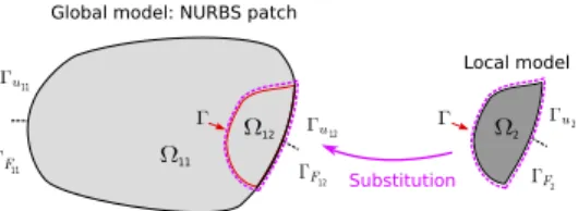
Fig. 3. The non-intrusive global/local problem.
With above notations, the resulting variational formulation of the coupled problem can be written as follows: Find u11∈U11, u2∈U2, and λ ∈ M such that:
a11(u11, v11) + b(λ, v11) = l11(v11) , ∀v11 ∈V11; a2(u2, v2) − b(λ, v2) = l2(v2) , ∀v2∈V2; b(µ, u11−u2) = 0, ∀µ ∈ M. (10)
Rather than directly solving Eq.(10)(i.e., in a monolithic way), an asymmetric algorithm, where Neumann problems over Ω11 and Dirichlet problems over Ω2are alternatively solved until convergence, may also be used. This leads to
the standard global/local algorithm. For the nth iteration, we can proceed as follows: starting withλ(0)∈M, we look for u11(n)∈U11, u2(n)∈U2, andλ(n)∈M such that:
1. Resolution of a Neumann problem over Ω11:
a11
u(n)11, v11
=l11(v11) − b(λ(n−1), v11), ∀v11 ∈V11. (11)
2. Resolution of a Dirichlet problem over Ω2:
a2 u(n)2 , v2 −b(λ(n), v2) = l2(v2) , ∀v2∈V2; b(µ, u(n)2 ) = b(µ, u(n)11), ∀µ ∈ M. (12)
The global/local algorithm (11)–(12) has the drawback to be intrusive. Indeed, it is important to note that the stiffness operator a11depends at this stage on the interface Γ or, in other words, on the shape of the local domain Ω2.
As a consequence, if domain Ω2has to evolve (during optimization process, or crack propagation for instance), not
only the local operator a2but also the global operator a11 have to be fully re-built and factorized. This can be very
time consuming and especially in the NURBS framework since the strategy would involve several re-parametrizations of the global NURBS patch. To overcome the difficulty, the purpose of this work is to make use of the non-intrusive coupling [27]. This is the object of the next section.
3. The global/local non-intrusive strategy 3.1. Principle
Rather than considering only a part of the NURBS patch (region Ω11) as the domain containing the global model,
the idea of non-intrusive coupling is to involve a global model defined over the whole existing NURBS patch. The situation is illustrated inFig. 3. In order to do this, domain Ω12is introduced to characterize the region in which the
global model of Ω11is fictively prolonged. Ω12is defined in such a way that the NURBS patch domain is covered by
Ω11∪Ω12. From here on, we refer to domain Ω1=Ω11∪Ω12to characterize the global NURBS patch that contains
the global model everywhere. We proceed in the same way with the boundaries by introducing Γu1 =Γu11∪Γu12for
the prescribed displacements and ΓF1 =ΓF11∪ΓF12for the applied forces. The objective of the non-intrusive strategy
is then to replace the global model over Ω12 by the local one in Ω2 without actually modifying the global NURBS
patch operators over Ω1.
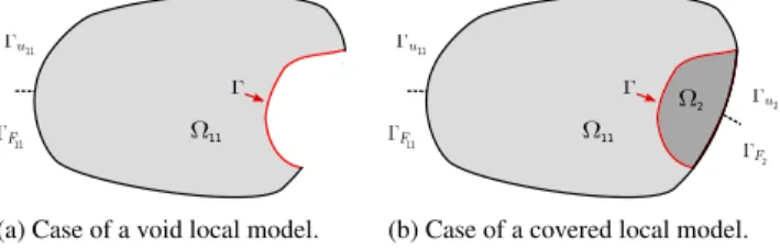
For the construction of the non-intrusive strategy, we proceed in two parts. Each of the parts has its own application. In the first part, we consider the particular case of the non-intrusive modelling of geometric details in a NURBS patch. Domain Ω2is then assumed to be a hole that is bounded by a trimming curve. In this case, the local model is said to
(a) Case of a void local model. (b) Case of a covered local model.
Fig. 4. Problems to be solved using the non-intrusive strategy.
be “void”. In the second part, we investigate the more usual situation of a covered local model that behaves differently from the global model. In contrast to “void” models, we refer to “covered” local models in the second case.Fig. 4
shows the problems to be solved for the two cases. 3.2. Part 1: case of “void” local models
3.2.1. The continuum version
In the case of a void local model (seeFig. 4(a)), the equations related to domain Ω2 vanish in the reference
problem(4)–(5). Taking into account these simplifications in Eq.(10)leads to the following usual weak form for the new problem:
Find u11 ∈U11such that:
a11(u11, v11) = l11(v11) , ∀v11∈V11.
(13) To derive the corresponding non-intrusive formulation, we first perform a continuous prolongation of the displacement solution from Ω11to Ω12. There are (in principle) infinitely many possible prolongations but an arbitrary prolongation
can be used for the formulation of the method. From a practical point of view, we define u1the prolongation of u11to
the full domain Ω1such that:
u1∈ H1(Ω1) d ⇔u1= u11∈ H1(Ω11) d u12∈ H1(Ω12) d and u11 |Γ =u12|Γ. (14)
u12 corresponds to the prolonged part of the global solution u1 to domain Ω12. As well, we introduce fg12 = fg2,
Fg12 = Fg2 and ug12 = ug2 the fictitious prolongation of f11g , Fg11 and ug11 to Ω12, ΓF12 and Γu12, respectively. In this
specific case of a void local model, we may take fg12 = 0, Fg
12 = 0 and u g
12 = 0. With these notations, we can
reformulate problem(13)over Ω1as follows:
Find u1∈U1such that:
a1(u1, v1) = a1(u1, v1) + {l11(v1) − a11(u1, v1)} , ∀v1∈V1,
(15) where the functional spaces U1and V1and the bilinear form a1are defined over Ω1using the formalism of Eqs.(6)
and(8), respectively. Then, we can make use of the additivity of the integral with respect to domain Ω1=Ω11∪Ω12:
a1(u1, v1) = a11(u1, v1) + a12(u1, v1) , ∀u1∈U1, ∀v1∈V1, (16)
which leads to the following simplification of Eq.(15):
Find u1∈U1such that:
a1(u1, v1) = l11(v1) + a12(u1, v1) , ∀v1∈V1.
(17) Finally, by writing the equilibrium of domain Ω12:
a12(u1, v1) = l12(v1) +
Γ
a1(u1, v1) = l1(v1) + Γ
σ12(u1) n12·v1dΓ, ∀v1∈V1.
(19)
For the resolution, a fixed point as in Eqs.(11)and(12)can be implemented. This time, only Neumann problems need to be solved. For the nth iteration, we proceed as follows: starting with u1(0)∈U1, we look for u(n)1 ∈U1such that:
a1 u(n)1 , v1 =l1(v1) + Γσ 12 u(n−1)1 n12·v1dΓ, ∀v1∈V1. (20)
Thanks to the prolongation of the global model over Ω12, the global operators a1and l1over Ω1are now involved
without any modification. During the iterations, only reaction forces across Γ need to be computed. In this sense, the strategy is said to be non-intrusive. In our case of a NURBS discretization, this may highly facilitate the modelling of geometric details since it avoids the complex task of constructing a new NURBS parametrization of the global model (and of re-constructing it each time the detail evolves).
3.2.2. The discrete version
Let us introduce the NURBS functions N1AA∈{1,2,...,n1} that discretize domain Ω1. Following the principle of
isoparametric elements, the basis N1AA∈{1,2,...,n1} is used to build the finite element space U1hcorresponding to the
discretization of U1. By substituting this NURBS approximation in the weak form Eq.(19)and performing as in
Eq.(20), we can derive the discrete non-intrusive algorithm. For the nth iteration, we proceed as follows: starting with {U1}(0), we look for {U1}(n)such that:
[K1] {U1}(n)= {F1} + { R12}(n−1). (21)
Operator [K1] (respectively {F1}) is the classical stiffness matrix (resp. vector force) associated to domain Ω1and,
{ R12} is introduced to denote the discrete reaction forces at Γ of the global model in the fictitious part (Ω12). The
convergence test usually performed to stop this algorithm relies on the discrete equilibrium of the reaction forces of the initial coupled problem at the interface Γ . Since in this case domain Ω2 is void, we simply need to verify that
the reaction forces at Γ of the global model in Ω11, denoted {R11}, are sufficiently close to zero. This leads to the
following definition of the interface equilibrium residual: ηvoid=
∥ {R11} ∥
∥ {F1} ∥ .
(22) It may be noted that the fictitious prolongation of the global solution over Ω12has no physical meaning (it depends
on the initialization). Moreover, it is important to notice that the algorithm proposed here is the standard one and that its convergence may be slow in certain situations. To answer this issue, acceleration techniques, such as based on an Aitken’s Delta Squared method or a Quasi-Newton method, can be applied to the present situation from the existing developments in classical FEM (see, e.g., [30]). Numerical experiments to account for this point will be carried out in Section4.
Remark 4. With its discrete version in hand (see Eq.(21)), the physics of the new problem may be easily understand-able. Indeed, roughly speaking, the new problem to be solved is a problem over Ω1that is subjected along Γ to a
surface force {R12}. As a consequence, performing the equilibrium of the new problem at Γ leads to:
{ R11} + { R12} = { R12} ⇒ { R11} = {0}, (23)
3.2.3. Implementation: computation of the interface reaction forces
The setting up of algorithm (21)requires the evaluation of the reaction forces {R12}. In order to be consistent
with the discrete approximations, {R12} has to be computed from its associated stiffness matrix and vector force as
follows:
{ R12} =([K12] {U1} − {F12}) |Γ. (24)
This implies performing a volume integral of the form: a12
uh1, vh1+l12
vh1 , (25)
and applying the restriction operator ·|Γ on a discrete vector. The restriction operator on Γ of a discrete vector {F } is defined such that:
{F } |Γ =[BΓ] {F }, (26)
where [BΓ] is the Boolean trace operator that selects only the degrees of freedom concerned by the interface. Remark 5. We emphasize that the computation of the reaction forces from a volume integral and not directly from a surface integral (as in Eq.(19)) is necessary to obtain a non-intrusive strategy in the discrete case as the finite element error is not taken into account otherwise. We specify that in the finite element setting, Eq.(18)becomes:
[K12] {U1} = {F12} +([K12] {U1} − {F12}) |Γ. (27)
Such a decomposition is usual in FEM non-intrusive coupling (see, e.g., [11,29,30]).
Although implementing the volume integral(24)–(25)is quite straightforward in FEM, the extension in the NURBS context may require additional attention. Conforming geometries are usually considered in FEM (see, e.g., [12,11,30]) whereas, due to the rigid tensor product structure of NURBS, non-conforming geometries need to be addressed in this work (there is no reason for the interface Γ to be aligned with the edges of the elements in Ω1). To perform
the calculation(24), a special integration scheme is required to evaluate the contribution of the global operators in Ω12 only. We recall that the only available data regarding Ω2 is the parametrization of the trimming curve that
forms its boundary ∂Ω2. For the general case, existing techniques could be used to define a suitable quadrature
rule: for instance, the standard sub-triangulation technique in the context of X-FEM [42], or the hierarchical element subdivision employed in the FCM [25,19,20], or the technique used in the NURBS Enhanced FEM [43]. Now, for most cases arising in the situation of geometric details, it seems that an exact NURBS domain may be simply constructed from the NURBS trimming curve by adding multiple interpolatory control points at the centre of the detail.
To illustrate the strategy, we return to the example ofFig. 1, namely a plate with a circular hole. The basis of our strategy is to construct a NURBS parametrization of the surface contained inside the circular curve (in red in
Fig. 1). Let us denote this surface (Ω12) by the disc and its boundary (Γ ) by the circular curve. To generate the disc
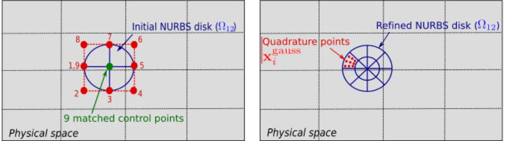
with NURBS, as many control points as necessary to define the circular curve (with the same weights as for the curve) can be put and matched together at the centre of the circular curve. The initial NURBS parametrization of the disc is composed of four elements of degree two in the circumferential direction and of degree one in the radial direction (seeFig. 5(a)). Then, usual NURBS mesh refinement techniques can be applied to produce a quadrature rule enabling the behaviour of the global model to be accurately seized in the disc Ω12(seeFig. 5(b) for a mesh of 8
(circumferential direction) ×2 (radial direction) elements with a 3 × 3 Gaussian rule per element). From the newly constructed NURBS parametrization of the disc, the standard integration rule for NURBS is used: p + 1 Gauss points ( p being the polynomial order) are considered in each direction per element. The last thing to be done is to pull back the quadrature points to the parametric domain of the plate (seeFig. 5(c)). This can be achieved simply by performing Newton–Raphson iterations to inverse the NURBS mapping:
xgaussi = n1 A=1 N1Aξgaussi x1A ⇒ ξgauss i . (28)
xgaussi denotes the coordinates of the quadrature points in the physical space andξgaussi refers to the corresponding coordinates in the parametric space. The advantage of the proposed technique is that it produces NURBS conforming
(a) Construction of the NURBS disc from the trimming curve.
(b) Refinement of the NURBS disc.
(c) Inverse mapping.
Fig. 5. Construction of a suitable quadrature rule for {R12}.
quadrature rules simply (in the sense that the quadrature points are aligned with the trimming curve that bounds the NURBS domain). Such a strategy applies directly to all types of star domains. Based on the same principle, we believe that most of the details of engineering interest can be generated with a few additional efforts. Corresponding investigations are in progress to generalize the procedure. We also note that new strategies producing conforming quadrature rules for trimmed surfaces have appeared very recently (see Nagy et al. [44] and Kudela et al. [45]) and may constitute promising options to be considered in our future works.
Remark 6. We emphasize that the NURBS mesh of Fig. 5(b) is only constructed here to produce an accurate integration rule for [K12] and {F12}. The corresponding stiffness operator is never assembled and factorized.
Furthermore, it may be noted that operators [K12] and {F12} are of small size (the NURBS function NA1, whose
support does not reach the small region Ω12, does not contribute), and can be computed in the pre-processing step.
As a result, the computation of the reaction forces only requires small-size matrix–vector products during the non-intrusive algorithm, which is not expensive.
Remark 7. With the above developments, the problem can be solved directly by performing:
([K1] − [K12]) {U1} = {F1} − {F12}. (29)
In this sense, the method can be classified as a fictitious domain approach and is very close to the so-called NURBS FCM [25,19,20], the only difference being the quadrature rule used. Rather than computing Eq.(29), we believe that the proposed non-intrusive strategy (Eq.(21)) may be more suitable for the modelling of geometric details that could evolve during the simulation. Independently of the shape of the geometric details, the global stiffness operator is assembled and factorized only once and the system to be solved remains well-conditioned. The price to pay is the number of iterations, but this can be strongly reduced by means of acceleration techniques.
Remark 8. Setting up the non-intrusive algorithm (21) also requires computation of the reaction forces {R11} to
evaluate the equilibrium residual(22). This is obtained from the already-computed stiffness [K12] and force {F12} as
follows:
3.3. Part 2: case of “covered” local models 3.3.1. The continuum version
The strategy proposed for geometric details can easily be extended to the modelling of covered local behaviours in a NURBS patch (i.e., when Ω2is not void but constitutes a real domain, seeFig. 4(b)). Indeed, going back to the
reference problem of Section2.2, exactly the same procedure as for a void local model can be applied to Eq.(11)to rewrite the Neumann problem over the whole NURBS patch Ω1. By doing that, the global/local non-intrusive
algo-rithm straightforwardly follows from the standard algoalgo-rithm(11)–(12). For the nth iteration, we start with u(0)1 ∈U1
andλ(0)∈M and we look for u(n)1 ∈U1, u(n)2 ∈U2, andλ(n)∈M such that:
1. Resolution of a Neumann problem over Ω1:
a1 u(n)1 , v1 =l1(v1) − b(λ(n−1), v1) + Γσ12 u(n−1)1 n12·v1dΓ, ∀v1∈V1. (31)
2. Resolution of a Dirichlet problem over Ω2:
a2 u(n)2 , v2 −b(λ(n), v2) = l2(v2) , ∀v2∈V2; b(µ, u(n)2 ) = b(µ, u(n)1 ), ∀µ ∈ M. (32)
Once again, the operators over the whole global NURBS patch are now involved in Eq.(31)without any modification and, only displacement and force exchanges at the interface Γ are required. This accounts for the non-intrusiveness of the strategy and thus, for the simplicity of the method to model local behaviours in a NURBS patch.
3.3.2. The discrete version
To derive the discrete version of the global/local non-intrusive algorithm(31)–(32), we need to introduce the approximation spaces U2h and Mh associated to U
2 and M, respectively. Keeping the principle of isoparametric
element, we consider for U2hthe basis functions N2 B
B∈{1,2,...,n2} that discretize domain Ω2. For the discretization of
the Lagrange multiplier space, special care may be required since bad-chosen basis can lead to undesirable energy-free oscillations (due to the non-satisfaction of the inf–sup condition). For the sake of simplicity, we adopt in this work a classical strategy (see, e.g., [30]): the trace along the coupling interface Γ of the basis functions of domain Ω2is
considered for Mh. With such a choice, we never encountered instabilities in our computations. The discrete version can then be written as follows: for the nth iteration, we start with {U1}(0)and {Λ}(0)and we look for {U1}(n), {U2}(n),
and {Λ}(n)such that:
1. Resolution of a Neumann problem over Ω1:
[K1] {U1}(n)= {F1} − [C1]T{Λ}(n−1)+ {R12}(n−1). (33)
2. Resolution of a Dirichlet problem over Ω2:
[K2] −[C2]T −[C2] [0] {U 2}(n) {Λ}(n) = {F 2} −[C1] {U1}(n) . (34)
[C1] and [C2] are the classical mortar coupling operators. To stop the algorithm, the global reaction forces at Γ ({R11})
have to be compared to the local reaction forces pulled back in Ω11, i.e. {R2} = [C1]T{Λ}. It leads to the following
equilibrium residual: ηcovered=
∥ {R11} + { R2} ∥
∥ {F1} ∥ .
(35) We emphasize that such an algorithm is classical in non-intrusive coupling and has been widely studied in the field of FEM. For more information, the interested reader is advised to consult Duval et al. [30] and references cited therein. Finally, the same remarks as for a void local model can be done about the algorithm. The fictitious prolongation of the global solution over Ω12 has no physical meaning and has to be replaced by the solution in Ω2. The number of
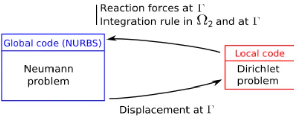
Fig. 6. The non-intrusive strategy: coupling of codes.
3.3.3. Implementation aspects
Since in this case the discretization of domain Ω2is explicitly known, we use it to simply compute the quadrature
rule required to evaluate the reaction forces {R12} of Ω12(and so {R11}, seeRemark 8). As well, we use the integration
rule coming from the discretization of the part Γ of the boundary∂Ω2for the computation of the coupling matrices
[C1] and [C2]. Since the global and local problems are solved alternatively in a non-intrusive strategy, two different
numerical codes can be used for the resolution (one for the global Neumann problem(33)and the other for the local Dirichlet problem(34)). This feature offers an important flexibility to the method. Indeed, if a linear NURBS code is used for the global NURBS problem, any other existing robust codes (NURBS, FEM, X-FEM, FCM) suitable for the modelling of complex behaviours (fracture, plasticity, contact) may be used to incorporate an accurate local model. The only need for that is to be able to apply Dirichlet boundary conditions to the local problem and to extract from its resolution the reaction forces at Γ and the quadrature rules in Ω2and over Γ (seeFig. 6for illustration). The local
model actually acts as a correction applied to the global model on the right-hand side. 4. Numerical results
We now present a range of numerical examples in two-dimensional linear elasticity in order to assess the performance of the proposed strategy. As in the previous section, the presentation is divided into two parts: first, the situation of a “void” local model is addressed in Section4.1; then, the more usual case of enrichment by a “covered” local model is investigated in Section4.2. We recall that the local model is said to be “void” when the associated region constitutes a hole, while the adjective “covered” is used to qualify a local model over the existing real region Ω2. Regarding the discretization of the global model, we start from a patch composed of a single element, to which we
apply the k-refinement strategy. Thus, the continuity across the interior knots is Cp−1, p being the polynomial degree of the NURBS functions. From here on, the mesh composed of N elements along the first length and M elements along the second length will be denoted N × M. In the illustrations, we keep the notations introduced in the previous section; in particular, domain Ω1=Ω11∪Ω12characterizes the global NURBS patch, the model of which in domain
Ω12is to be replaced either by a void model or by another discrete model contained in domain Ω2.
4.1. Modelling of geometric details
In this first part, the methodology implemented is the one related to Section 3.2. Our interest here is in how geometric details are modelled. Two numerical examples are investigated. In the first one, where an analytical reference solution is available, we illustrate that our non-intrusive methodology does not compromise accuracy and that few iterations are required, especially when acceleration techniques are used. In the second example, we illustrate the potential of the method to treat more complex cases of geometric details.
4.1.1. Infinite plate with a circular hole
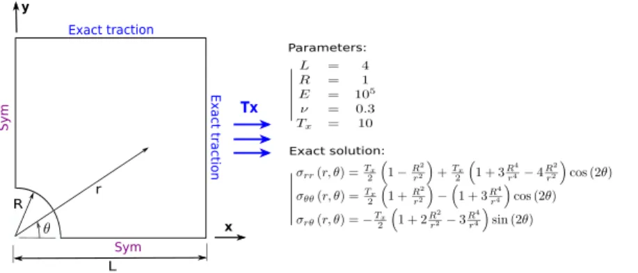
Description of the test case: To start with, the popular example of an infinite plate with a circular hole under in-plane tension is considered. The geometry, material, boundary conditions and the analytical solution [46] are given inFig. 7. Because of symmetry, the problem is restricted to one quarter of the plate. This problem was among the first to be studied with NURBS [1,2] and was later investigated in the framework of the fictitious domain concept [14]. The discretization of the problem following the non-intrusive strategy developed is illustrated inFig. 8(a). A regular B-Spline mesh is used for the plate without the hole (domain Ω1) and a circular NURBS mesh is constructed to produce
Fig. 7. Infinite plate with a circular hole: description and data of the problem.
the derivation of the quadrature rule: the associated stiffness operator is never assembled and factorized. For a curved domain, the first length (where there are N elements) is the circumferential length and the second length (discretized by M elements) is the radial length. This notation also holds for the following examples.
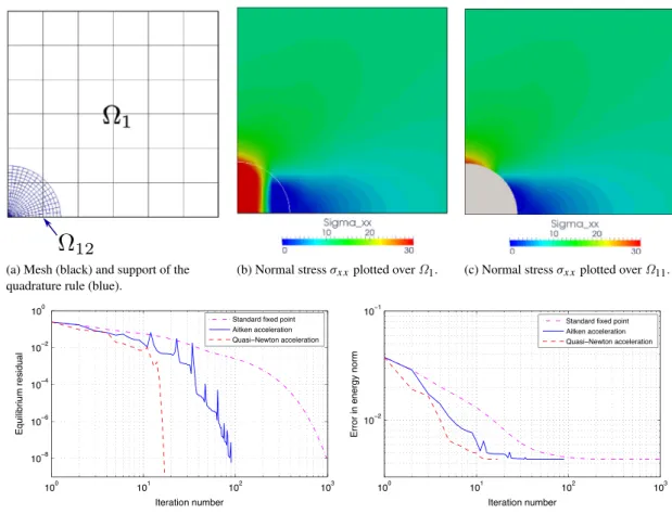
Study of the non-intrusive algorithm: First, the behaviour of the non-intrusive algorithm(21)is studied. The results obtained with the discretization ofFig. 8(a) are grouped inFig. 8(b)–(e). More precisely,Fig. 8(b) and (c) show plots of the normal stress in the horizontal x-direction obtained (once the algorithm has converged) in the embedded domain Ω1 and in the true domain Ω11, respectively. Removing the smooth non-physical fictitious prolongation in
Ω12, the solution appears to be in good agreement with Refs. [1,2,14].Fig. 8(b) and (c) enable the convergence of the
iterative algorithm to be appreciated: first, in terms of the equilibrium residual (Eq.(22)) and then in terms of the error on the displacements in energy norm. Note that the error is computed by taking only contributions in Ω11into account.
The standard fixed point and also Aitken’s Delta squared and Quasi-Newton acceleration techniques are implemented. The equilibrium residual falls to zero, which accounts for the convergence of the algorithm. Conversely, the error on the displacement reaches an asymptotic value, which corresponds to the NURBS finite element approximation. As noted inRemark 7, the use of acceleration techniques strongly reduces the number of iterations: the number of iterations needed to attain the finite element accuracy, which seems to be obtained for a residual of about 10−3, is reduced by a factor of ten in this example.
Remark 9. By comparingFig. 8(d) and (e), it may be noted that reaching a residual as low as 10−8is probably not necessary to achieve an accurate numerical solution. Nevertheless, as the development of efficient convergence criteria was not the purpose of the present contribution, we kept a value of 10−8for the equilibrium residual to stop the algorithm. Thus the number of iterations required is probably overestimated.
Study of the finite element convergence: Then, the convergence of the method with respect to the mesh size is studied. Here, the non-intrusive algorithm is performed until convergence. To get a general view,Fig. 9shows plots of the normal stress in the horizontal x-direction for different cubic B-spline meshes of the global patch, which can be directly compared to corresponding plots given in [14]. No visible difference with [14] can be observed. To go further, the convergence behaviour of the displacements in the energy norm under uniform refinement is plotted inFig. 10, starting from a mesh of 4 × 4 B-spline elements for the global model. Polynomial degrees p = 1, p = 2 and p = 3 are considered in both spatial directions. We note that the NURBS mesh of the hole needs to be sufficiently fine to give a suitable quadrature rule for the interface reaction forces. We use a NURBS mesh composed of 50 × 50 elements for the finer B-spline mesh of the global model. The optimal rates of convergence of hpare seen to be achieved (h being the characteristic element size), which demonstrates that the methodology does not interfere with the accuracy of the NURBS functions.
4.1.2. Perforated strip under tension
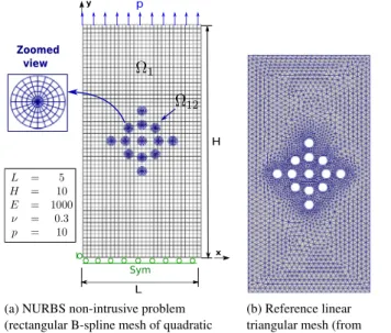
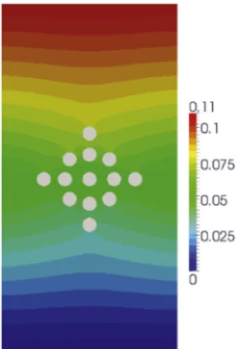
Description of the test case: To illustrate the robustness of the method, the more complex case of a plane strip perforated in its middle part by several holes and subjected to constant in-plane tension is now computed. The numerical model is described inFig. 11(a). Note that such a test case is usually encountered in the field of immersed boundary methods (see, e.g., [19]). In our non-intrusive model, a regular quadratic B-spline mesh is used for the global
(a) Mesh (black) and support of the quadrature rule (blue).
(b) Normal stressσx xplotted over Ω1. (c) Normal stressσx xplotted over Ω11.
(d) Convergence of the interface equilibrium residual. (e) Convergence of the displacements in the energy norm.
Fig. 8. Non-intrusive analysis of the infinite plate with a circular hole (rectangular B-spline mesh of quadratic 6 × 6 elements for Ω1+circular NURBS mesh of quadratic 15 × 15 elements for the quadrature rule in Ω12). (For interpretation of the references to colour in this figure legend, the reader is referred to the web version of this article.)
(a) 3 × 3 elements. (b) 6 × 6 elements. (c) 12 × 12 elements.
Fig. 9. Normal stressσx x, plotted over Ω11, for different cubic B-spline meshes.
model of the plate without the holes and each hole is specified by a circular NURBS mesh. We emphasize that the interest of the method here is the simplicity with which it handles a modification of the perforation (size and number of holes). For comparison purposes, a refined finite element solution is computed using the classical linear triangular elements implemented in Code Aster [47]. The corresponding boundary fitted discretization is shown inFig. 11(b).
Fig. 10. Convergence of the displacement in the energy norm, when the B-spline grid is uniformly refined.
(a) NURBS non-intrusive problem (rectangular B-spline mesh of quadratic 30 × 60 elements for Ω1+13 circular NURBS meshes of quadratic 20 × 5 elements for the quadrature rule in Ω12).
(b) Reference linear triangular mesh (from Code Aster).
Fig. 11. Perforated tensile specimen.
Numerical results: The results are given inFig. 12.Fig. 12(a)–(c) show, respectively, the displacement in the x-direction, the displacement in the y-direction and the von Mises stress obtained with the non-intrusive model of
Fig. 11(a). The same information is plotted inFig. 12(d)–(f) for the reference FE solution. The two solutions are very close, which shows the accuracy of the non-intrusive methodology. The horizontal and vertical displacements exhibit a necking effect due to the stiffness reduction induced by the perforations and the typical stress concentration phenomena around the holes are well represented. Finally, the convergence of the non-intrusive algorithm can be observed in Fig. 12(g): a residual of 10−4 is obtained in about 20 iterations and approximately 30 iterations are required to reach a residual of 10−8.
4.2. Modelling of local behaviours
In this second part, we illustrate the behaviour of the proposed non-intrusive strategy when applied to covered local models. The developments established in Section3.3are implemented here and three examples are considered. In the first, the strategy is used to perform NURBS local refinement on a simple test case, which demonstrates that the non-intrusive coupling method does not compromise accuracy. The second example concerns applications to
(a) NURBS non-intrusive disp. ux.
(b) NURBS non-intrusive disp. uy. (c) NURBS non-intrusive Von Mises stressσvm.
(d) FE reference disp. ux. (e) FE reference disp. uy. (f) FE reference VM stress σvm.
(g) Convergence of the interface equilibrium residual.
Fig. 12. Non-intrusive analysis of the perforated strip under tension and comparison with a reference FE solution.
micromechanics of materials. In particular, the ability of the method to treat a plate with a stiffer inclusion is shown. Finally, the non-intrusive coupling of two different types of elements (NURBS and FEM) coming from two different numerical codes is performed to model a crack in a NURBS patch.
(a) Problem description and discretization. (b) Displacement field (magnitude).
(c) Von Mises stress. (d) Error of the Von Mises stress (normalized by the maximum VM stress).
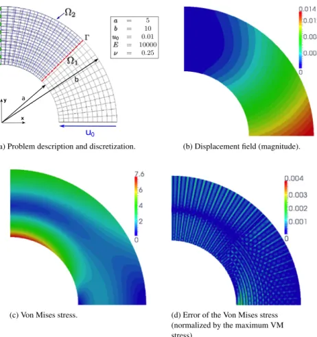
Fig. 13. Non-intrusive analysis of the curved beam problem (NURBS mesh of quadratic 25 × 12 elements for Ω1(12.5 × 12 elements for Ω11) + NURBS mesh of quadratic 12 × 20 elements for Ω2).
4.2.1. Curved beam subjected to end shear
Description of the test case: The first example consists of a curved beam subjected to end shear. The problem, together with its non-intrusive discretization, is illustrated inFig. 13(a). A constant radial displacement of u0=0.01
units is prescribed over the lower beam boundary. An analytical solution for a reference plane stress model is available for the problem in [48]. The same polynomial order is used in both spatial directions and for the global model as well as for the local model. A minimum order of p = 2 is necessary to represent the curvature exactly. In the upper half of the structure, the global NURBS model is meant to be replaced by a more refined (along the radial direction) NURBS model. We posit that the material properties are the same for the global and local models, the only difference being the mesh size. In order to address the coupling of non-conforming geometries, an odd number of elements along the circumferential direction is considered for the global patch. Such a choice leads to an interface Γ that cuts (in the middle) a layer of elements of the global model.
Numerical results
• The results obtained (once the non-intrusive algorithm has converged) with the discretization ofFig. 13(a) are shown in terms of displacement inFig. 13(b) and in terms of Von Mises stress inFig. 13(c) and (d). The Von Mises error is normalized by the maximum reference Von Mises stress encountered in the domain. We emphasize that it is the coupling solution in Ω11∪Ω2that is mapped (the fictitious prolongation of the global solution over Ω12is not
represented). The solution corresponds to Ref. [48] (error of the Von Mises stress less than 0.4%, seeFig. 13(d)). In particular, there is no visible error concentration around the coupling interface Γ .
• To better appreciate the accuracy of the method, we study the convergence of the coupling solution with the refinement of the mesh (seeFig. 14). We proceed in the same way as in Ref. [48]: the convergence behaviour
Fig. 14. Convergence of the strain energy for uniform refinement in both subdomains.
Table 1
Meshes considered to study the convergence behaviour.
Number of elements Single-patch Coupled discretization
(Nel) mesh (Ω11∪Ω2)
24 (=N1el) 6 × 4 3.5 × 3 ∪ 3 × 5
96 12 × 8 6.5 × 6 ∪ 6 × 10
384 24 × 16 12.5 × 12 ∪ 12 × 20
1536 32 × 48 24.5 × 24 ∪ 24 × 40
of the strain energy is considered. The relative energy error is computed as: |Edex−Edf e|
Edex , (36)
where Edex denotes the reference exact strain energy and Edf e the strain energy of the NURBS finite element model. Orders p = 2 and 3 are investigated. To refine the non-intrusive coupling solution, we consider the meshes indicated inTable 1(right column). For each approximation, the first mesh discretizes domain Ω11 (this is the
global mesh divided in half along the circumferential direction; that is why half of the elements are involved) and the second mesh is used for domain Ω2 (this is the local mesh). We note that the refinement obtained between
successive meshes is not exactly uniform since there are always some elements of the global model that are cut. For comparison purposes, the convergence curves of (almost) equivalent single-patch solutions have been added in
Fig. 14. Also, the equivalent single-patch meshes are reported inTable 1(middle column). Finally, the convergence curves are plotted with respect to the equivalent number of elements Nel normalized by the number of elements N1elof the equivalent coarsest mesh (see left column ofTable 1for the associated values).
• We observe that the rate of convergence and the error constant of the non-intrusive coupled discretizations are equivalent to those of the equivalent patch discretization. True, a slight discrepancy appears since the single-patch model cannot exactly represent the non-conforming coupled model. For the finest cubic single-single-patch mesh, the error level is so low that it may be deteriorated by rounding errors. These results indicate that the error coming from the non-intrusive coupling methodology is significantly smaller than the error due to the NURBS finite element approximation. This means that the accuracy of NURBS is preserved with the proposed methodology when applied to covered local models.
4.2.2. Plate with a central inclusion
Description of the test case: With the next example, the situation of a non-conforming covered local model that has different material properties from those of the global model is investigated, considering the modelling of a plate with a central inclusion subjected to constant in-plane tension (seeFig. 15). Note that such types of test cases have already been computed using an embedded Nitsche’s method (see, e.g., [9]). Here, the proposed non-intrusive
(a) First model: local model = inclusion. (b) Second model: local model = inclusion + annulus.
Fig. 15. Plate with a central inclusion: description and discretization of the problem.
coupling strategy is implemented. In order to be different from the situation of holes (where, roughly speaking, the local stiffness equals zero) and to be consistent with composite materials, the Young’s modulus is chosen to be a hundred times larger for the inclusion than for the plate (Ei =100 × Ep). The Poisson’s coefficients are the same.
Numerical models considered: Two different numerical non-intrusive models are considered for the problem (see
Fig. 15(a) for the first model andFig. 15(b) for the second one). For each, a regular quadratic B-Spline grid is used for the global model and a circular quadratic NURBS mesh is constructed for the local model. However, in the first situation, the local model includes the inclusion only, while in the second case, an annulus of two elements in the radial direction is added at the boundary of the inclusion to constitute the local model. In the second local model, two different materials separated by a C0continuity then need to be considered to recover the solution of the initial problem: Ei is taken at the centre (i.e., in the inclusion) and Epis fixed in the annulus. By doing this, we will see that
we are able to achieve good accuracy with relatively coarse meshes for the plate. The transition of the solution from the local model to the global one across Γ becomes smoother in the second situation while sharp phenomena need to be correctly captured in the first model. The difference of mesh size in the plate to obtain an equivalent solution with the first model and the second model is illustrated and reported inFig. 15.
Numerical results
• The results obtained once the non-intrusive algorithm has converged are given inFig. 16(a)–(c) for the first model andFig. 16(d)–(f) for the second situation. The first plots are related to the discretization ofFig. 15(a) and the second plots concern the discretization ofFig. 15(b). For both models, the vertical displacement, the vertical strain and the Von Mises stress are shown. The solutions of the two models are in good agreement. The stiffer behaviour of the inclusion seems to be well captured: the vertical strain is low while the Von Mises stress is high in the inclusion. • The associated convergence behaviour of the non-intrusive algorithm is given inFig. 17. As already observed in the framework of non-intrusive coupling in FEM, the Newton acceleration technique appears to be necessary to reach convergence in the situation of a local model stiffer than the global model. Furthermore, we observe that the convergence is much slower for the first model (seeFig. 17(a)) than for the second model (seeFig. 17(b)) where the usual number of several tens of iterations is reached. The reason for this is the difference of stiffness between the global (fictitious) model in Ω12and the local model in Ω2. Theoretically, this can be shown by rewriting the fixed
point as a modified Newton algorithm where the approximation of the tangent matrix depends on the gap in the primal Schur complements between the models in Ω12and in Ω2(see, e.g., [30]). To conclude on these results, the
two non-intrusive models implemented enable the problem to be solved accurately. Nevertheless, we emphasize that, for better convergence of the algorithm, the primal Schur complement of the local model (Dirichlet problem with prescribed displacement on Γ ) has to be relatively close to the primal Schur complement of the global model in Ω12. This is consistent with the original idea of global/local non-intrusive coupling: the region of the local model
(a) Model 1: disp. uy. (b) Model 1: strainεyy. (c) Model 1: VM stressσvm.
(d) Model 2: disp. uy. (e) Model 2: strainεyy. (f) Model 2: VM stressσvm.
Fig. 16. Plate with a central inclusion: converged solution of the non-intrusive analysis (top: first model, bottom: second model).
(at its centre) and larger regions (at its boundaries) where the connection with a simpler global model can be made efficiently.
4.2.3. Edge-cracked plate under uniaxial tension
Description of the test case: In the last example, we demonstrate the ability of the proposed methodology to combine analysis models that consist of several different element types coming from different numerical codes. In particular, we are interested in the coupling of NURBS elements with standard finite elements (i.e., based on Lagrange shape functions). This may be of great interest for engineers because it provides a flexible tool to couple robust conventional finite element codes with newly developed NURBS codes. We recall that the procedure illustrated inFig. 6is used for the non-intrusive coupling. For the study, an edge-cracked plate, as shown inFig. 18(a), subjected to a uniform tensile stress is analysed. The crack size (a = 1) is very small in comparison with the lengths of the plate (H = 17 and L = 7), so the problem exhibits two different scales. The structure is assumed to be in plane strain conditions. Such a problem has already been studied in the context of non-intrusive FEM (see, e.g., [11]). The reference value of the mode I Stress Intensity Factor (SIF) can be accurately approximated by the value that holds for
(a) First model: interface equilibrium residual. (b) Second model: interface equilibrium residual.
Fig. 17. Convergence of the non-intrusive algorithm for the plate with a central inclusion.
an infinite plate, corrected by a factor depending on the ratio aL:
Kr e fI =p √ aπ1.12 − 0.231a L +10.55 a L 2 −21.72 a L 3 +30.39 a l 4 . (37)
Numerical model considered: The non-intrusive numerical model considered is illustrated inFig. 18(b). To model the behaviour around the crack, we propose to make use of the well-established X-FEM method (in the context of usual FEM). In particular, X-FEM linear triangles are used here to discretize the local model. In addition, we propose to add an analytical domain at the crack tip in the local model, which contains the Williams’ expansion [49]. The consequence of this is that the stress intensity factors can be derived directly. For details regarding crack modelling, the interested reader is invited to consult [11] and references cited therein. The local model is computed using the code of [11]. Simultaneously, a quadratic 15×30 B-spline mesh is used in our IGA code as the global model to compute the plate without the crack. This model is intended to be replaced around the crack by the local model presented above. Non-conforming geometries are involved (see, again,Fig. 18(b)).
Numerical results: The vertical displacement obtained (once the non-intrusive algorithm has converged) with the discretizations ofFig. 18(b) is plotted inFig. 18(c). A deformation similar to that in [11] can be observed. In addition, the convergence behaviour of the mode I SIF KI with the non-intrusive algorithm is shown inFig. 19. We note
that only five iterations are required to obtain the converged value with the Newton acceleration technique. For the discretization considered, a relative error of 0.08% on KI with respect to Kr e fI (Eq.(37)) is reached. These results
account for the flexibility of the method to connect finite element methods that use different basis functions. The present work can then be interpreted as an extension of the non-intrusive coupling coming from conventional FEM to higher-order finite element methods.
5. Conclusion
In this paper, we applied the global/local non-intrusive coupling strategy to the NURBS context in order to simplify the modelling of local behaviour within a NURBS patch. The idea was to consider the NURBS patch to be enriched as the global model. The first advantage of the methodology when applied to NURBS is that the global NURBS patch remains unchanged, which completely eliminates the need for costly re-parametrization procedures, even if the local domain is expected to evolve during the simulation. In addition, it should be emphasized that the global stiffness operator is assembled and factorized only once, and the system to be solved remains well-conditioned. The second advantage of the proposed approach is its considerable flexibility. Beyond being an efficient strategy to couple different element types, the formalism offers the possibility to couple different numerical codes with very little implementation effort. Since the global and local problems are solved alternately and only interface data are transmitted in a non-intrusive strategy, it is possible to use a linear NURBS code for the global model and any other existing robust codes suitable for the modelling of complex behaviour for the local model. This notably allows for easy merging of robust conventional FEM codes with newly developed NURBS codes which, in our opinion, may foster the integration of NURBS in the engineering world.
(a) Problem description. (b) Meshes: global quadratic B-Spline model (the local region in grey) and local model including X-FEM linear triangles (crack in red) and the analytical domain (black).
(c) Converged solution: disp. uy.
Fig. 18. Non-intrusive analysis of an edge crack plate under uniaxial stress. (For interpretation of the references to colour in this figure legend, the reader is referred to the web version of this article.)
Fig. 19. Convergence of the SIF KI during the non-intrusive algorithm.
We have presented a range of numerical examples that demonstrate the ability of the non-intrusive coupling to model various types of local behaviour within a NURBS patch. Starting with the specific case of a local model that is void, we derived a strategy for the situation of geometric details, which requires only global Neumann problems to be solved in the iterative procedure. In a second part, we investigated the more usual case of covered local models. First, we considered a refined NURBS local model to achieve local refinement, then studied the modelling of a stiffer inclusion by involving a local model with a different Young modulus and, finally, combined our linear NURBS code with a standard FEM code to incorporate a local model including standard X-FEM linear triangles for crack modelling. The results confirm that the proposed approach does not compromise accuracy. In particular, the optimal rates of convergence were achieved. The price to pay for the non-intrusive strategy is the number of iterations of the solver but we have shown that this can be reduced to a few dozen with the use of acceleration techniques (Aitken dynamic relaxation and Quasi-Newton update). In consequence, we believe that our methodology is of significant interest for treating any case of local enrichment expected to evolve in a NURBS patch.
From the non-intrusive coupling point of view, the main development from FEM to NURBS consisted of taking non-conforming geometries into account. Because of the rigid tensor product structure of NURBS, the case of a local