O
pen
A
rchive
T
OULOUSE
A
rchive
O
uverte (
OATAO
)
OATAO is an open access repository that collects the work of Toulouse researchers and
makes it freely available over the web where possible.
This is an author-deposited version published in :
http://oatao.univ-toulouse.fr/
Eprints ID : 17999
To link to this article : DOI:10.1016/j.matcom.2016.08.009
URL :
http://dx.doi.org/10.1016/j.matcom.2016.08.009
To cite this version : Zaibi, Malek and Champenois, Gérard and
Roboam, Xavier and Belhadj, Jamel and Sareni, Bruno
Smart power
management of a hybrid photovoltaic/wind stand-alone system
coupling battery storage and hydraulic network.
(2016) Mathematics
and Computers in Simulation, vol. 146. pp. 210-228. ISSN 0378-4754
Item availablity restricted.
Any correspondence concerning this service should be sent to the repository
administrator:
[email protected]
Smart power management of a hybrid photovoltaic/wind stand-alone
system coupling battery storage and hydraulic network
Malek Zaibi
a,b,∗, G´erard Champenois
a, Xavier Roboam
c, Jamel Belhadj
b, Bruno Sareni
caLIAS, Universit´e de Poitiers, LIAS-ENSIP, B25, TSA 41105 86073 Poitiers cedex 9, France bLSE, Universit´e de Tunis El Manar, ENIT BP 37, 1002 Tunis Le Belv´ed`ere, Tunisia cLAPLACE, Universit´e de Toulouse, ENSEEIHT, 2 Rue Camichel 31071 Toulouse Cedex, France
Abstract
An off-grid energy system based on renewable photovoltaics (PV) and wind turbines (WT) generators is coupled via converters to electric and hydraulic networks. The electric network is composed of consumers and of a battery bank for electrical storage, while the hydraulic part is made of motor-pumps and hydraulic tanks for water production and desalination. Both battery and water tanks are used to optimize the power management of both electric and hydraulic subsystems by ensuring electric load demand and by reducing at the same time water deficit following the operation of the renewable intermittent source. Thus, both electric and hydraulic subsystems are strongly coupled in terms of energy making necessary to manage the power flows provided by renewable sources to optimize the overall system performance. In this paper, two kinds of management strategies are then compared in the way they share the hybrid power sources between the storage devices (battery and tanks) and the electrical/hydraulic loads. The first approach deals with an “uncoupled power management” in which the operation of electrical and hydraulic loads does not depend on the state of the intermittent renewable sources: in particular, hydraulic pumps are operated only taking account of water demand and tank filling but without considering power sources. On the contrary, given the available power produced by the sources, the second class of strategy (i.e. the “coupled management strategy”) consists of a “smart” power sharing between the electrical and hydraulic networks with regard to the battery SOC and the tank L1and L2. A dynamic simulator of the hybrid energy
system has been developed and tested using a MATLAB environment. The system performance is shown under the two investigated approaches (uncoupled vs coupled). Several tests are carried out using real meteorological data of a remote area and a practical load demand profile. The simulation results show that the “coupled strategy” clearly outperforms the classical “uncoupled” management strategies.
Keywords:Hybrid energy system; Battery storage; Hydraulic storage; Dynamic simulator; Smart power management
1. Introduction
Off-grid power supply systems based on renewable energies are of great interest for applications such as remote areas electrification, telecommunication station powering, water pumping and/or desalination for irrigation
∗Corresponding author at: LIAS, Universit´e de Poitiers, LIAS-ENSIP, B25, TSA 41105 86073 Poitiers cedex 9, France.
E-mail address:[email protected](M. Zaibi). http://dx.doi.org/10.1016/j.matcom.2016.08.009
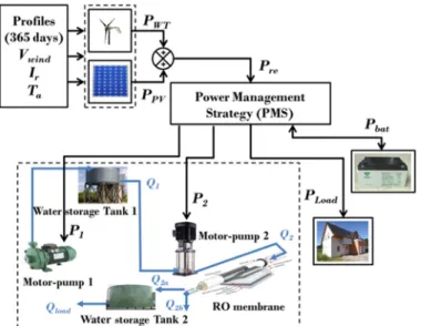
Fig. 1. Global system architecture.
or drinking. These systems usually exploit the coupling between photovoltaic (PV) and wind generators [3] but can also be coupled to conventional generators such as diesel generators [35,23,24], hydrogen storage [18,9,36,33], fuel cells [28,2,20,16,17,40], micro–hydro generators [6,7,27,29] and batteries [30,4,24,20,14,1,40]. In this paper, a hybrid off-grid supply system including PV and wind generators with battery storage is studied for producing electricity and water from pumping and desalination. In such devices, the use of a Power Management System (PMS) is of prime importance for optimal operation and represents a key element of the system. Many alternative power management strategies can be used to manage an off-grid hybrid energy system. In [11], the mixed-integer linear programming models are used to perform the energy management of off-grid hybrid power systems with renewable sources. In [13], a mathematical model has been used for the energy management based on short-term generation scheduling with the aim of determining at each step the status of the overall microgrid giving the minimum operating costs. In [39], the authors have developed real and reactive power management strategies of electronically-interfaced distributed generation for a Microgrid with energy storage systems. In [22,5], different power management strategies based on logical block diagrams have been developed for a stand-alone power system with load and battery and hydrogen storage. Likewise, [15] suggests for the same system a power management based on a state machine approach. In addition, for renewable energy integration with power generation and water desalination, [27] introduces an energy management which takes random variations in demand and energy supply into account.
Nevertheless, limited research investigations have been reported with the energy management of water pumping systems from intermittent renewable sources [19]. For example, in [38] the hybrid system is studied but the power management is not given.
Thus, three PMS are investigated in this paper with various logic scenarios and operation cases which have been developed. The rest of the paper is organized as follows: In Section 2, the system configuration is defined and the models of components employed for each subsystem are briefly described. Section3 is devoted to the power management strategies aiming at optimizing the power and water flows. Section 4 reports the simulation results and the analysis of the system performance under various power management. Finally, conclusions are drawn in Section5.
2. System configuration and modeling
Fig. 1 shows the configuration of a hybrid PV/wind generator coupled with two kinds of storage i.e. electric (battery) and hydraulic (tanks) devices.
The meteorological profiles: wind speed(Vwind), solar irradiation (Ir) and ambient temperature (Ta) of a typical
region in Tunisia have been recorded for one year. The power flow Pr e drawn from the hybrid PV/WT sources is
Predictions of load demand and renewable source powers are often assessed in smart grids to optimize power management and to minimize storage capacity. The source/load prediction is in particular exploited in micro grids as in smart cities [31] or in island grids [8]. In this paper, we have focused on the typical case of a standalone system in an isolated farm fully powered from renewable sources; in such applications, prediction tools are often not available and the hypothesis of a non-predictable load and source powers has been made. In such cases, heuristics are classically used to manage power flows in the system as presented in the paper. Such heuristics have to face correctly the intermittent nature of PV and wind generation but are clearly sub optimal with respect to global scheduling methods that optimize trajectories from the knowledge of information prediction: the dynamic programming is an example of such approaches.
A dynamic simulator has been developed using MATLAB/Simulink⃝R environment. In this dynamic simulator, six subsystems are implemented: the PV generator, the wind turbine, the battery storage, the electrical load, the hydraulic network and the PMS. As illustrated on Fig. 1, the hydraulic network is composed of 2 motor-pumps for water pumping and desalination, a high pressure pump (motor-pump 2) connected to a reverse osmosis desalination device (“RO membrane”).
2.1. Hybrid energy source models
Regarding the objectives of this study, i.e. setting the energy management strategies and progressing towards the integrated design of the whole electro-hydraulic network according to long term (typ. 1 year) environment profiles, system modeling is limited to power flow models. Therefore, quasi-static power flow models with compact computing time are considered; such low granularity levels are enough accurate especially to assess power management issue, taking account of energy efficiency of coupled devices. This choice of model class aims at facilitating system analysis and to optimize the whole system on a very wide time horizon taking into account both environment (solar irradiation and wind speed) profiles, and assignments for electric and hydraulic loads.
2.1.1. PV generator model
The solar irradiation(Ir) and the ambient temperature (Ta) measurements are used to calculate the output power
of the PV generator.
Several models can be found in the literature to estimate the PV generator power [12,5,15]. This PV generator power is determined from model as defined in [21,26]:
PP V =ηr ·ηpc· [1 −β · (Tc−N OC T)] · AP V ·Ir (1)
whereηr is PV efficiency,ηpcthe power tracking equipment efficiency (which is equal to 0.9 with a perfect maximum
point tracker),β the temperature coefficient (ranging from 0.004 to 0.006 per◦C for silicon cells), N OC T is normal operating PV cell temperature (◦C), AP V the PV panels area (m2) and Tcthe PV cell temperature (◦C) which can be
expressed by [25]:
Tc=30 + 0.0175 · (Ir−300) + 1.14 · (Ta−25) (2)
where Tadenotes the ambient temperature (◦C).
2.1.2. Wind turbine model
Through aerodynamic conversion, the wind power captured by a wind turbine is proportional to the swept area Awt, the air mass densityρ and the wind speed (Vwind).
To estimate the output power of wind turbine, the latter power is limited by a coefficient of power Cpdepending
on the ratioλ (λ = R · ω/Vwind, where R is the radius of the blades,ω is the speed angle of the turbine) and β is the blade pitch angle [15].
In order to simplify the model, the optimal value is used of the coefficient of power Cp, such as Cp=Cp,opt.
In this case, the wind turbine power is expressed as follows [34]:
PW T =
1
2 ·Cp,opt·ρ · Awt·V
3
2.1.3. Battery storage model
Several authors have proposed models for the battery and the results of experiments carried out on lead/acid batteries deduce a model named “CIEMAT model” representing the battery operation during the charge, discharge and overcharge processes. In our case study, from the carried out experiments, a validated model is proposed with respect to the battery capacity for any size and type of lead/acid battery [10].
This model represented by an equivalent circuit model contains a voltage source which is the open circuit voltage V0, in series with an internal resistance r . Thus, the output voltage of the battery is VBat =V0±IBat·r where the
both VBatand IBat depend on the battery state of charge(SOC), temperature and internal resistance variations r.
In this study, this simple model based on the CIEMAT model for the battery is considered as enough accurate to assess power management objectives and to compare performance of several strategies. During the charging and discharging process, the state of charge(SOC) vs time (t) can be described by [1]:
SOC(t) = SOC(t − ∆t)+ PBat· η ch Cn·Ubus ·∆t SOC(t − ∆t)+ PBat· 1 ηdi s·Cn·Ubus ·∆t (4)
where ∆t is the time step (here, half an hour), PBat represents the battery power determined by the PMS, Cnis the
nominal capacity of the battery,ηchandηdi sare respectively the battery efficiencies during charging and discharging
phase. Ubus denotes the nominal DC bus voltage. At any time step ∆t , the SOC must comply with the following
constraints:
SOCmi n≤SOC(t) ≤ SOCmax (5)
where SOCmi nand SOCmaxare maximum and minimum allowable storage capacities, respectively.
2.1.4. Electrical load profile
Typical power consumption data Pload were acquired for a residential home. During 365 days with half an hour
acquisition period, this profile describes a weekday and weekend day consumption. 2.2. Hydraulic network models
The hydraulic network is shown inFig. 1. It includes four principal subsystems: the motor-pump 1 which draws water from well, a water storage tank 1, the high pressure motor-pump 2 associated with a reverse osmosis desalination device. A water tank storage 2 is finally placed at the output of the desalination process to store fresh water.
The proposed models are quasi-static models which performances have been previously compared and validated with reference to dynamic models using Bond-Graph formalisms [32].
2.2.1. Model of the motor-pump 1
The GRUNDFOS⃝R motor-pump model CRN-3-10’s nominal power was selected for pumping water from well to the tank water storage 1. The rated motor-pump power is 0.75 kW. The characteristics H(Q1) and the efficiency
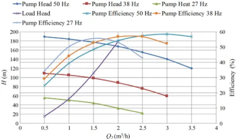
curve of the motor-pump 1 for two frequencies 50 Hz and 40 Hz and the load characteristic Hload(Q1) are shown in Fig. 2. The operating point of pumping is the crossing point between H(Q1) and Hload(Q1). A weak variation of the
motor-pump frequency (i.e. 40 Hz) decreases the pump efficiency. For this reason, we use the optimal operation of pump 1 with a fixed frequency (i.e. 50 Hz). The electric power P1required for motor-pump 1 at head H and flow rate
Q1can be calculated as [37]:
P1= ρw
·g · H · Q1
ηm·ηp
(6) whereρw is the density of water (kg/m3), g the gravity constant (m/s2),ηm the motor efficiency andηpthe pump
Fig. 2. Hydraulic characteristics of motor-pump 1.
2.2.2. Model of the water storage tank 1
Water tank 1 is used to store brackish water. It is characterized by its water level L1and its section S1. The level
L1can be calculated as follows:
L1(t) = L1(t − ∆t) +(Q1(t) − Q2(t))
S1
·∆t. (7)
This tank is fitted with four sensors measuring four different water levels: two minimum sublevels, i.e. high and low (L1,minH and L1,minL) and two maximum sublevels, i.e high and low (L1,max H and L1,max L). The high and low
levels are separated by a hysteresis band. This hysteresis avoids the switch on/off of the motor-pump during operation. 2.2.3. Model of the motor-pump 2
The GRUNDFOS⃝R motor-pump model CRN-3-29 was selected for water pumping from the tank water storage 1 to the tank water storage 2 via a reverse osmosis (RO) desalination system. The rated motor-pump power is 2.2 kW. Contrary to the case of the motor-pump 1, this motor-pump can operate at variable frequencies whilst maintaining a good level of efficiency (seeFig. 3). It is interesting to match the energy availability with the power of pump 2 for maximizing water production. The pump head pressure must be greater than the osmotic pressure.Fig. 3presents three characteristics H(Q2) with the efficiency curves of motor-pump 2 for the corresponding frequencies: 50 Hz,
38 Hz and 27 Hz, and also the load characteristic Hload(Q2). By satisfying the previous constraints, the
motor-pump 2 frequency varies between 50 Hz and 27 Hz. The expression of the flow rate Q2is a function of the electric
power P2.
Q2= −2, 17.10−7·P22+10, 7.10 −4·P
2+0, 683 (8)
where P2corresponds with the electric power required for the motor-pump 2 at each duty point from 27 Hz to 50 Hz.
For the RO process, the flow rate Q2is divided into the permeate flow Q2a and the concentrate flow Q2b. These two
flows are depend on the pressure P2and are defined as follows [37]:
P2= (Rvalve+Rmodule) · Q22b Q2a= P2 Rmembr ane Q2= Q2a+Q2b (9)
where Rmembr ane, Rmodule and Rvalve are the hydraulic resistances of the membrane, the module and the valve,
Fig. 3. Hydraulic Characteristic of Motor-pump 2.
2.2.4. Modeling of the fresh water storage tank 2
Water storage tank 2 is the tank of permeate (fresh) water. It is defined by the level L2and section S2. The level L2
can be calculated as follows: L2(t) = L2(t − ∆t) +(Q
2a(t) − Qload(t))
S2
·∆t (10)
where Qload is the water flow demand required by the consumers. As previously, this tank is fitted with four level
sensors: two useful levels, i.e. high and low (L2,uH and L2,uL) and two maximum levels, i.e. high and low (L2,max H
and L2,max L). The high and low levels are also determined by a hysteresis band.
3. Power management strategies
3.1. Description of the power management strategies
The hybrid renewable power generation obtained under the weather conditions should be capable of providing power for the electrical and hydraulic loads. Hence, the battery and the water tanks will be used to compensate or reduce both the electric energy and water deficits during the system operation in its environment. The key indicators that govern the operation of the system are the SOC of battery and levels of both tanks, i.e. L1and L2.
Two approaches can be suggested to share the renewable source power between the electrical and hydraulic loads: • Approach 1: “Uncoupled power management strategy”
The policy of this approach is to meet the electrical and hydraulic loads following their demands (i.e. the electrical and water demands) and whatever the state of the intermittent power production.
In this approach, the operation of electrical and hydraulic loads does not depend on the intermittent power production but only on their demands (i.e. electrical and water demands). In this case, to satisfy the water demand, the motor-pumps are operated with the nominal power following the tank filling levels (i.e. level L1for
motor-pump 1 and level L2for motor-pump 2). This operation is similar to a “flushing operation” and corresponds to the
classical way of hydraulic load management: powering a pump to fill the tank only when its low limit is reached. But in reality, the energy availability is limited by the intermittence of PV and wind sources and the battery capacity. Consequently, two strategies are developed to manage the state of charge(SOC) of the battery according to the need of the electrical/hydraulic loads. In strategy 1, the electrical load is privileged before the hydraulic loads and conversely for strategy 2 where the hydraulic loads is privileged. In other words, available power from sources and battery is used for electric loads then for hydraulic pumps in the strategy 1 and conversely for the strategy 2. Thus, in both strategies the load management does not depend on the state of renewable sources. In this case,
Fig. 4. Diagram of the hydraulic load power operation.
the battery must be sized in terms of power and energy to compensate the unbalance between the source and the requested loads.
In the strategies 1 (PMS 1: E +) and 2 (PMS 2: H +), the hydraulic network is seen as a whole electric load. The standard operations of the motor-pumps 1 and 2 are determined with respect to the tank filling levels (L1and
L2). If The level (L1and L2) are between Lmi net Lmax, the motor-pumps (P1and P2) are operated according the
F1 and F2 functions. If L2 < L2,min with L1 > L1,min, then P2is matter of priority. If L1< L1,min, then P1is
matter of priority and P2is stopped. The flowchart of the hydraulic load power operation is presented inFig. 4.
Thus, for the strategies 1 and 2, the input is the rest power ∆P which can be calculated as follows:
∆P = Pr e−[PLoad+P1+P2]. (11)
If the battery SOC is high enough, the electrical and hydraulic loads run according to requirements, and the battery can provide or absorb the ∆P if this latter is inside the power range of the battery. If the SOC of battery is low : – Strategy 1(E+): the need of the electrical load is the priority while the pumps are switched off.
– Strategy 2(H+): the need of the hydraulic power is privileged and the electrical load is switched off. • Approach 2: “Coupled power management strategy” (PMS 3: C)
In this approach, the management evolutes according to the variation of the intermittent power production. Therefore, strategy 3 is developed for a smart management of the hybrid system, coupling power source, the battery, the electrical load and the pump power (P1and P2) according to the battery SOC and the tank levels L1
and L2. The power P2can be modulated between two power limits to limit the power exchanged with the battery.
The input of this strategy is the difference power PDi f f. PDi f f corresponds to the remaining power calculated by
the difference between the source power(Pr e) and the load electric power Pload(see Eq.(12)).
PDi f f = Pr e−PLoad. (12)
For every range of PDi f f, several scenarios are studied in terms of the battery SOC and tank storage levels (L1and
3.2. Definition of system indicators
To estimate the performance of different power management strategies in this complex system, the following system indicators are used:
1. The Loss of electric Power Supply Probability(LPSPE):
LPSPE(%) = 100 · T ∆t=1 |δP(∆t)| · ∆t T ∆t=1 Pload(∆t) · ∆t (13)
whereδP account for “Non-fulfillment” of electricity production. 2. The Loss of hydraulic Power Supply Probability(LPSPH):
LPSPH(%) = 100 · T ∆t=1 [Qload(∆t) · ∆t]L2(∆t)=0 Qload·T . (14)
3. The Excess of Production(E P):
E P(%) = 100 · T ∆t=1 PE x cess(∆t) · ∆t T ∆t=1 Pr e(∆t) · ∆t (15)
where PE x cessis the power excess not used for loads or for electrical and hydraulic storage.
4. The exchange energy by the battery(Eex):
Eex(%) = 100 · T ∆t=1 | PBat(∆t)| · ∆t T ∆t=1 Pr e(∆t) · ∆t (16)
where PBatis the battery power.
5. The electric losses of the system(Losses):
Losses(%) = 100 · T ∆t=1 [Pr e−(P1+P2+PLoad+PE x cess)] (∆t) · ∆t T ∆t=1 Pr e(∆t) · ∆t (17)
where P1and P2are, respectively, the electric power of motor-pumps 1 and 2.
Finally, three strategies of power management are suggested for the system, and the flowchart of any of these three power management strategies is presented in the following subsections.
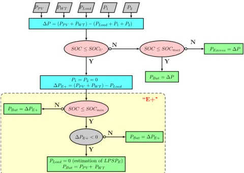
3.3. Power management strategy 1 (PMS 1: E +)
In this strategy, we remind that the electrical load is privileged over the hydraulic loads.
The different cases of PMS 1 are grouped inFig. 5. The PMS 1 depends on the magnitude of ∆P, the battery state of charge(SOC) and the levels of the tank 1 and 2 (L1and L2).
• Case 1. SOC(t) < SOCU
Fig. 5. Flowchart of Power Management Strategy 1: uncoupled PMS where the electrical load is privileged(E+).
If SOC(t) ≤ SOCmi nthen:
– if ∆PE +≥0 then the electrical load power Ploaddoes operate and the battery charges with PBat =∆PH +.
– if ∆PE +≤0 then the production is not sufficient(Pload =0) and the LPSPEincreases withδP = PLoadduring
the occurrence of “case 1” and the battery charges with PBat =Pr e.
If SOC(t) > SOCmi nthen the battery discharges or charges with PBat =∆PE +.
• Case 2. SOC(t) ≥ SOCU
The battery discharges or charges with PBat = ∆P. The electrical load power (Pload) is functional and the
hydraulic load power (P1and P2) operates depending on the flowchart given inFig. 4.
If the battery is full(SOC(t) > SOCmax), then the power excess (PE x cess) is calculated with
PE x cess =∆P.
In all cases, if the tank 2 is empty(L2=0) the loss of hydraulic power supply probability LPSPH is calculated.
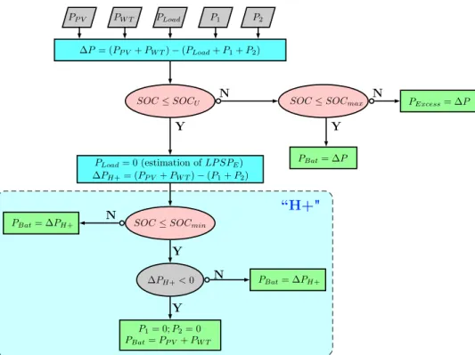
3.4. Power management strategy 2 (PMS 2: H +)
Conversely to the previous strategy, the hydraulic loads is privileged over the electrical load.
The flowchart for PMS 2 is shown inFig. 6. Similarly, the PMS 2 depends on the magnitude of ∆P, the battery state of charge(SOC) and the levels of the tank 1 and 2 (L1and L2).
• Case 1. SOC(t) < SOCU
The electrical load power is null(PLoad =0), the LPSPEincreases withδP = PLoadduring the occurrence of
“case 1” and ∆PH + =Pr e−(P1+P2).
If SOC(t) ≤ SOCmi nthen:
– if ∆PH + ≥ 0 then the hydraulic load power (P1 and P2) is functional and the battery charges with PBat =
∆PH +.
– if ∆PH + ≤0 then the production is not sufficient(P1=P2=0) and the battery charges with PBat =Pr e.
If SOC(t) > SOCmi nthen the battery discharges or charges with PBat =∆PH +.
• Case 2. SOC(t) ≥ SOCU
In this case and similarly to PMS 1 (“case 2”), The battery discharges or charges with PBat =∆P. The electrical
load power(Pload) is functional and the hydraulic load power (P1and P2) operate depending on the flowchart given
Fig. 6. Flowchart of Power Management Strategy 2: uncoupled PMS where the hydraulic load is privileged(H+).
If the battery is full(SOC(t) > SOCmax), then the excess power (PE x cess) is calculated with
PE x cess =∆P.
In all cases, if the tank 2 is empty(L2=0) the loss of hydraulic power supply probability LPSPH is calculated.
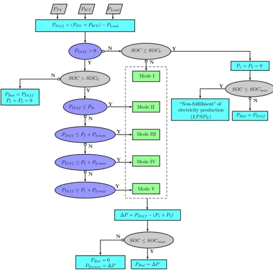
3.5. Power management strategy 3 (PMS 3)
The core of this paper is the algorithm of sharing renewable energies between the two pumps and storage in the battery to ensure the electric and water consumptions with maximum satisfaction. So, this algorithm takes into account the levels of the three storages (SOC of the battery, L1and L2respectively levels of the tanks 1 and 2) according to
the renewable energy fluxes. For efficiency, the pump 2 works also with speed-controllers. First, management is done following the result of the remaining power when the electric charge is deducted from renewable electrical power generated: PDi f f =PW T +PP V −PLoad.
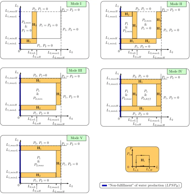
The flowchart of this coupled power management strategy 3 is shown inFig. 7. According to the importance of the amplitude of PDi f f and the SOC of the battery, five modes are developed taking into account the water levels in the
two tanks. The first mode is when PDi f f is negative. The four others modes(PDi f f > 0) depend of the level of PDi f f
with the threshold level calculated with the power pumps: P1, P2,min and P2,max (with P1: nominal power of pump
1, P2,min and P2,max the power levels of pump 2 in speed-controlled limits).Fig. 8shown this five modes.
In this strategy, the hysteresis bands are used to prevent the switching on/off of the power P1and the power P2in
different cases of tank levels 1 and 2 as follows (seeFig. 8):
• H1: a hysteresis band to eliminate the switching on/off of the power P1.
• H2: a hysteresis band to eliminate the switching on/off of the power P2
3.5.1. PDi f f negative
• Scenario (a):(PDi f f < 0)
If the SOC is greater than SOCU then the battery discharges, it is the mode I: P1 or P2 work to obtain the
Fig. 7. Flowchart of Power Management Strategy 3: the coupled PMS.
If the SOC is smaller than SOCUand greater than SOCmi nthen the electric load is operated. Also, if the SOC is
smaller than SOCmi nthen the production cannot be satisfied and the LPSPEincreases with PDi f f. In the both last
cases no power is sent towards the hydraulic system.
Note than, in any case, if the tank 2 is empty(L2 =0) the loss of hydraulic power supply probability LPSPH is
calculated.
3.5.2. PDi f f positive
For all the following scenarios, if battery SOC is less than the “useful state of charge” SOCU, then PDi f f is used
to charge the battery: PBat = PDi f f with the electric load is operated and the pumps are stopped. Also, both tank 1
and tank 2 are full, the power PDi f f is equal to PBator PE x cess if the battery is full.
SOCU is a typical level of the SOC that gives the preference to storing PDi f f in the battery instead of using it for
the hydraulic load. This strategy then aims at minimizing the LPSPE criterion while limiting the depth of discharge
(DO D) for maximizing battery life.
The usage level L2,uis chosen to favor the fresh water availability, so as to minimize the LPSPH criterion.
• Scenario (b):(0 < PDi f f < Pt h)
The power Pt his defined the maximal threshold between the minimal power of motor-pump 2(P2,min) and the
power of motor-pump 1(P1) (i.e. Pt h=max P2,min, P1).
If the SOC is smaller than SOCmax then the mode II is operational with P1and P2,min can work together to
Fig. 8. Diagram of PMS 3 for different modes of hydraulic load operation.
P2,min (small speed) and with L1> L1,min. The rest power ∆P = Pdi f f −P1−P2is stored in the battery with
PBat=∆P.
If the SOC is greater than SOCmax, then the battery is full and ∆P is lost. In this case, a coefficient of excess of
production E P is returned. This coefficient is computed from the excess power(PE x cess=∆P).
Note than for all the following scenarios, when the battery is full(SOC > SOCmax) the same conditions are
met.
• Scenario (c): Pt h < PDi f f < P1+P2,min
If the SOC is smaller than SOCmax then the mode III is operational with P1and P2can work together if the max
level of each tank is not reach and L1> L1,min and the battery discharges with PBat = PDi f f −P1−P2,min. In
this mode, P2is limited at P2,min (small speed).
• Scenario (d): P1+P2,min < PDi f f < P1+P2,max If the SOC is smaller than SOCmax then the mode IV is
operational. If tank 2 is empty or lower than a usage level L2,uand tank 1 is not empty(L1> L1,min) then PDi f f
Table 1
System parameters for the three PMSs.
AP V AW T Cn/UBat
60 m2 30 m2 800 Ah/48 V
P1 P2,min P2,max
796 W 314 W 1863 W
if tank 2 is upper than a usage level L2,u and tank 1 is not empty(L1 > L1,min) then PDi f f is used for pump 1
(P1) and pump 2 (P2=P2,di f f) with P2,di f f =PDi f f −P1and PBat =0.
• Scenario (e):(PDi f f > P1+P2max) If the SOC is smaller than SOCmax then the mode V is operational. The
two pumps can operate together with the maximum speed for the pump 2 and if L1 > L1,min. In this case, the
remaining power PDi f f −(P1+P2,max) is positive.
4. PMS performances
In this section, simulation results of the hybrid PV-Wind-Battery system in different power management strategies are presented.
For every PMS, the initial parameters are similar and use the dynamic simulator; simulations were carried out in order to validate the PMS performances under different strategies for one year of simulation with two different sites: the reference Tunisian and the American site.
The two sites have different characteristics: the first has a good solar irradiance and also a good wind site. The second is only a good solar site with a good regularity. So, for validate our management strategy, it is important to test on in different sites.
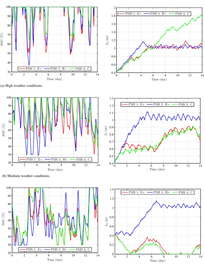
The dynamic simulator of the hybrid system is tested with different scenarios for the three strategies. To illustrate the evolution of system parameters (tank level L2and the battery SOC) a first simulation has be done during only 14
days, with Tunisian site data (i.e. wind speed(Vwind), solar irradiation (Ir) and ambient temperature (Ta)), in three
cases of weather conditions: • Case 1: High weather conditions • Case 2: Medium weather conditions • Case 3: Low weather conditions.
Fig. 9shows the three cases of renewable power recovered. In the first case with high weather conditions, the mean and the standard deviation of renewable power are respectively ⟨Pr e⟩ =6843 W, σPr e =5369 W. For medium weather conditions, the mean and the standard deviation of renewable power are respectively ⟨Pr e⟩ =3336 W, σPr e =3226 W. In the third case with minimum weather conditions, the mean and the standard deviation of renewable power are respectively ⟨Pr e⟩ =2378 W, σPr e =2457 W.
InTable 1, the parameters are presented to simulate the system using the dynamic simulator. Similarly,Table 2
presents the different parameters for the three PMS such as the initial parameters of tank levels L1and L2, and battery
SOC, the fixed values of threshold for tank levels L1and L2and battery SOC, the nominal power of motor-pump 1
and the range power of motor-pump 2 between the minimal and maximum powers.
Fig. 10shows the results of the tank level L2and the battery state of charge(SOC) vs time (with a ten minutes
sampling an horizon of 14 days) for the uncoupled strategies (PMS 1, PMS 2) and for the coupled strategy PMS 3. Similarly,Fig. 11shows the evolution of the loss of electric and hydraulic power supply probability LPSPE and
LPSPH with three weather conditions. Note that the loss hydraulic power supply probability LPSPH is null for the
three PMS with for medium and high conditions.
Thus, L2is maximized with PMS 2 in two of three cases, but for this management, when the SOC is lower than
SOCU (i.e. 65%), the LPSPE is increased (i.e. seeFig. 11). So, PMS 2 is not a good solution. PMS 1 and PMS
3 are similar solutions for the waveforms, but for L2, the PMS 3 management gets a better level in good weather
conditions and often a better battery SOC. This first result show the advantage of PMS 3 which leads to a better management of the power production. Indeed, when the tank level L2and the battery SOC do not reach their minimal
2.5 2 1.5 1 0.5 0 0 2 4 6 8 10 12 14 × 104 20000 18000 16000 14000 12000 10000 8000 6000 4000 2000 0 0 2 4 6 8 10 12 14
(a) High weather conditions. (b)Medium weather conditions.
14000 12000 10000 8000 6000 4000 2000 0 0 2 4 6 8 10 12 14
(c) Low weather conditions.
Fig. 9. Zoom during 14 days of the evolution of the renewable power Pr ewith three weather conditions.
Table 2
Control parameters of the three PMSs.
SOCmi n SOCU SOCmax
30% 65% 100%
Parameters of PMS 1 and PMS 2
L1,minL L1,minH L1,max
0.2 m 0.4 m 2 m
L2,min L2,max
1 m 2 m
Parameters of PMS 3
L1,minL L1,minH L1,max L L1,max H 0.2 m 0.4 m 1.8 m 2 m L2,minU L2,maxU L2,max L L2,max H 0.9 m 1.1 m 1.8 m 2 m
This first result show the advantage of the coupled PMS 3 strategy which leads to a better management of the power production.
100 90 80 70 60 50 40 30 0 2 4 6 8 10 12 14 0 2 4 6 8 10 12 14 2 1.8 1.6 1.4 1.2 0.8 0.6 0.4 1
(a) High weather conditions.
70 100 90 80 60 50 40 30 20 0 2 4 6 8 10 12 14 0 2 4 6 8 10 12 14 1.3 1.2 1.1 0.9 0.8 0.7 0.6 0.5 0.4 1
(b) Medium weather conditions.
70 100 90 80 60 50 40 30 20 0 2 4 6 8 10 12 14 0 2 4 6 8 10 12 14 1.4 1.2 0.8 0.6 0.4 0.2 1 0
(c) Low weather conditions.
Fig. 10. Evolution of the battery SOC and the tank level L2for different weather conditions during 14 days.
The second illustration is given byFig. 12. It is the synthesis results for one year,Fig. 12(a) for Tunisian site and
(a) LPSPEfor high weather conditions. (b) LPSPEfor medium weather conditions.
(c) LPSPEfor low weather conditions. (d) LPSPHfor low weather conditions.
Fig. 11. Zoom during 14 days of the evolution of the loss of electric and hydraulic power supply probability LPSPEand LPSPHwith three weather
conditions.
Fig. 12displays the performance indicators: the loss of electric and hydraulic power supply probability (LPSPE
and LPSPH), the excess of production(E P), the exchange energy by the battery (Eex) and the electric losses of the
system(Losses) for different management strategies.
The simulation results show significant differences between the power management strategies as shown inFig. 12. We can see in Fig. 12(a) for the reference Tunisian site, that the system indicators of the PMS 3 are better in comparison with those of the PMS 1 and PMS 2. Indeed, the loss of electric power supply probability(LPSPE) of the
PMS 3 is very small compared to the PMS 1 and PMS 2 (i.e. 1.06% for PMS 3 over 2.47% for PMS 1 and 29.16% for PMS 2). Also, the loss of hydraulic power supply probability(LPSPH) of the PMS 3 is very small (i.e. 1.34%)
compared to those found by PMS 1 (i.e. 2.74% for PMS 1).
The exchange energy with the battery is very important for the aging of the battery that has the consequence to increase the number battery replacements. So with PMS 3, the exchange are very limited (17.56%) than the two others (25%) and it is a major point for the PMS 3 management.
The excess energy of the PMS 3 is little higher to the PMS 1 (i.e. 41.73% for PMS 3 over 41.24% for PMS 2) and small to the PMS 2 (i.e. 48.34%) but the electric losses is smaller compared to the PMS 1 and 2 with 3.54% for PMS 3 over 4.54% for PMS 1 and 4.39% for PMS 2.
To confirm these results on other sites,Fig. 12(b) for the American site show that the system indicators of the PMS 3 are overall better in comparison with those of the PMS 1 and PMS 2 except the result of the loss of hydraulic power supply probability(LPSPH) where the PMS 2 is ideal compared to the PMS 3 (i.e. 0% for PMS 2 over 3.21% for
PMS 3).
To conclude,Fig. 12shows that PMS 3 clearly outperforms PMS 1 and PMS 2. PMS 1, which gives priority to the electrical load, presents a quite similar loss of electric power supply probability(LPSPE) but the loss of hydraulic
power supply probability(LPSPH) is more important. Similarly, PMS 2 which gives priority to the hydraulic loads,
(a) Performance using the reference Tunisian site.
(b) Performance using the American site.
Fig. 12. Performance of power management strategies for two different sites.
Thus, the smart management of tank storage levels and variation of the motor-pump power 2 between P2mi n and
P2max, better maintains hydraulic efficiency with variable power on motor pump 2 in this power range and allows
5. Conclusion
In this paper an off-grid hybrid PV/wind/ battery system consisting of an electrical load (power consumption for a residential home) and hydraulic load (water pumping and desalination) has been studied. Firstly, the system configuration, the component models and three power management strategies devoted to hybrid energy systems have been presented. Furthermore, a dynamic simulator has been developed using a MATLAB environment in order to assess the performance of the different power management strategies. The first two management strategies (PMS 1 and PMS 2) were elementary approaches which respectively gave priority to the electrical/hydraulic loads but which are not coupled with the renewable intermittent sources operation: in other words, both electric and hydraulic loads are only switched on in case of electric power demand or when tanks have to be filled, whatever the source state. A third “coupled” strategy (PMS 3) was proposed with the aim of performing a smart sharing of the hybrid power source between the electrical/hydraulic loads regarding simultaneously the battery SOC and the tank levels. Simulations over a long period of time (1 year) for two sites have shown the efficiency of this method which clearly outperforms the two classical management approaches by reducing hydraulic and electric losses and by increasing the quantity of produced water: it means that the hydraulic storage capacities (tanks) are better exploited from the “coupled vision of management” which better filters the intermittent source by “storing water in tanks better than ions in the electrochemical battery bank”. Finally, the presented system can constitute an interesting benchmark for testing optimal energy management methods and assessing their performance with regard to a reference constituted by the smart strategy PMS 3 proposed in this work.
Acknowledgments
The authors acknowledge the CMCU UTIQUE Program for financial support. This work was supported by the Tunisian Ministry of High Education and Research under Grant LSE-ENIT-LR 11ES15.
References
[1] D. Abbes, A. Martinez, G. Champenois, Life cycle cost, embodied energy and loss of power supply probability for the optimal design of hybrid power systems, Math. Comput. Simulation 98 (2014) 46–62.
[2] A. Abdelkafi, L. Krichen, Energy management optimization of a hybrid power production unit based renewable energies, Int. J. Electr. Power 62 (3–5) (2014) 1–9.
[3] R. Akikur, R. Saidur, H. Ping, K. Ullah, Comparative study of stand-alone and hybrid solar energy systems suitable for off-grid rural electrification: A review, J. Renew. Sustain. Energy. Rev. 27 (2013) 738–752.
[4] M.N. Ambia, A. Al-Durra, C. Caruana, S. Muyeen, Power management of hybrid micro-grid system by a generic centralized supervisory control scheme, J. Energy Convers. Manag. 8 (3) (2014) 57–65.
[5] M.S. Behzadi, M. Niasati, Comparative performance analysis of a hybrid pv/fc/battery stand-alone system using different power management strategies and sizing approaches, Int. J. Hydrogen Energy 40 (1) (2015) 538–548.
[6] M. Benghanem, K. Daffallah, S. Alamri, A. Joraid, Effect of pumping head on solar water pumping system, J. Energy Convers. Manag. 77 (2014) 334–339.
[7] M. Benghanem, K. Daffallah, A. Joraid, S. Alamri, A. Jaber, Performances of solar water pumping system using helical pump for a deep well: A case study for Madinah, Saudi Arabia, J. Energy Convers. Manag. 65 (2013) 50–56.
[8] L. Bridier, D. Hernandez-Torres, M. David, P. Lauret, A heuristic approach for optimal sizing of ess coupled with intermittent renewable sources systems, Renew. Energy 91 (2016) 155–165.
[9] G. Cau, D. Cocco, M. Petrollese, S.K. Kær, C. Milan, Energy management strategy based on short-term generation scheduling for a renewable microgrid using a hydrogen storage system, J. Energy Convers. Manag. 87 (1) (2014) 820–831.
[10] J. Copetti, F. Chenlo, Lead/acid batteries for photovoltaic applications. test results and modelling, J. Power Sources 47 (1994) 109–118. [11] R. Dai, M. Mesbahi, Optimal power generation and load management for off-grid hybrid power systems with renewable sources via
mixed-integer programming, J. Energy Convers. Manag. 73 (5) (2013) 234–244.
[12] A. Daud, M.S. Ismail, Design of isolated hybrid systems minimizing costs and pollutant emissions, J. Renew. Energy 44 (2012) 215–224. [13] M.Z. Daud, A. Mohamed, M. Hannan, An improved control method of battery energy storage system for hourly dispatch of photovoltaic
power sources, J. Energy Convers. Manag. 73 (2013) 256–270.
[14] E. Dursun, O. Kilic, Comparative evaluation of different power management strategies of a stand-alone pv/wind/pemfc hybrid power system, Int. J. Electr. Power 34 (2012) 81–89.
[15] D. Feroldi, L.N. Degliuomini, M. Basualdo, Energy management of a hybrid system based on wind–solar power sources and bioethanol, J. Chem. Eng. Res. Des. 91 (8) (2013) 1440–1455. special Issue: Computer Aided Process Engineering (CAPE) Tools for a Sustainable World.
[16] D. Feroldi, L.N. Degliuomini, M. Basualdo, Energy management of a hybrid system based on windsolar power sources and bioethanol, J. Chem. Eng. Res. Des. 91 (2) (2013) 1440–1455.
[17] D. Feroldi, D. Zumoffen, Sizing methodology for hybrid systems based on multiple renewable power sources integrated to the energy management strategy, Int. J. Hydrogen Energy 39 (2) (2014) 8609–8620.
[18] D. Giaouris, A.I. Papadopoulos, C. Ziogou, D. Ipsakis, S. Voutetakis, S. Papadopoulou, P. Seferlis, F. Stergiopoulos, C. Elmasides, Performance investigation of a hybrid renewable power generation and storage system using systemic power management models, J. Energy 61 (9) (2013) 621–635.
[19] C. Gopal, M. Mohanraj, P. Chandramohan, P. Chandrasekar, Renewable energy source water pumping systems—a literature review article, J. Renew. Sustain. Energy. Rev. 25 (2013) 351–370.
[20] H. Hemi, J. Ghouili, A. Cheriti, A real time fuzzy logic power management strategy for a fuel cell vehicle, J. Energy Convers. Manag. 80 (3) (2014) 63–70.
[21] J. Hofierka, J. Ka ˚Auk, Assessment of photovoltaic potential in urban areas using open-source solar radiation tools, J. Renew. Energy 34 (10) (2009) 2206–2214.
[22] D. Ipsakis, S. Voutetakis, P. Seferlis, F. Stergiopoulos, C. Elmasides, Power management strategies for a stand-alone power system using renewable energy sources and hydrogen storage, Int. J. Hydrogen Energy 34 (16) (2009) 7081–7095. 4th Dubrovnik Conference4th Dubrovnik Conference.
[23] A. Kaabechea, R. Ibtiouenb, Techno-economic optimization of hybrid photovoltaic/wind/diesel/battery generation in a stand-alone power system, J. Solar Energy 103 (2014) 171–182.
[24] S. Koohi-Kamali, N. Rahim, H. Mokhlis, Smart power management algorithm in microgrid consisting of photovoltaic, diesel, and battery storage plants considering variations in sunlight, temperature, and load, J. Energy Convers. Manag. 84 (6) (2014) 562–582.
[25] F. Lasnier, T.G. Ang, Photovoltaic Engineering Handbook, first ed., Taylor and Francis, 1990.
[26] B. Liu, S. Duan, T. Cai, Photovoltaic dc building module based bipv system: Concept and design considerations, IEEE Trans. Power Electron. 26 (5) (2011) 1418–1429.
[27] A. Mohammedi, N. Mezzai, D. Rekioua, T. Rekioua, Impact of shadow on the performances of a domestic photovoltaic pumping system incorporating an mppt control: A case study in Bejaia, North Algeria, J. Energy Convers. Manag. 84 (2014) 20–29.
[28] Z. Mokrani, D. Rekioua, T. Rekioua, Modeling, control and power management of hybrid photovoltaic fuel cells with battery bank supplying electric vehicle, Int. J. Hydrogen Energy 39 (5) (2014) 15178–15187.
[29] C. Moulay-Idriss, B. Mohamed, Application of the dtc control in the photovoltaic pumping system, J. Energy Convers. Manag. 65 (2013) 655–662.
[30] A. Nguyen, J. Lauber, M. Dambrine, Optimal control based algorithms for energy management of automotive power systems with battery/supercapacitor storage devices, J. Energy Convers. Manag. 87 (1) (2014) 410–420.
[31] R. Rigo-Mariani, X. Roboam, B. Sareni, Fast power flow scheduling and sensibivity analysis for sizing a micro-grid with storage, Math. Comput. Simulat. 131 (2017) 114–127.
[32] X. Roboam, B. Sareni, T.N. Duc, J. Belhadj, Optimal system management of a water pumping and desalination process supplied with intermittent renewable sources, in: Conf. IFAC PPPSC Toulouse, 2012.
[33] S. Safari, M. Ardehali, M. Sirizi, Particle swarm optimization based fuzzy logic controller for autonomous green power energy system with hydrogen storage, J. Energy Convers. Manag. 65 (2013) 41–49.
[34] W. Shepherd, D.W. Shepherd, Energy Studies, second ed., Imperial College press, 2003.
[35] H. Tazvinga, B. Zhu, X. Xia, Energy dispatch strategy for a photovoltaic–wind–diesel–battery hybrid power system, J. Solar Energy 108 (2014) 412–420.
[36] J.P. Torreglosa, P. Garc´ıa, L.M. Fern´andez, F. Jurado, Energy dispatching based on predictive controller of an off-grid wind turbine/ photovoltaic/hydrogen/battery hybrid system, J. Renew. Energy 74 (2015) 326–336.
[37] M. Turki, J. Belhadj, X. Roboam, Control strategy of an autonomous desalination unit fed by pv-wind hybrid system without battery storage, J. Electr. Syst. 4 (2008) 1–12.
[38] B.D. Vick, B.A. Neal, Analysis of off-grid hybrid wind turbine /solar pv water pumping systems, J. Solar Energy 86 (2012) 1197–1207. [39] K. Xian-guo, L. Zong-qi, Z. Jian-hua, New power management strategies for a microgrid with energy storage systems, J. Energy Procedia 16
(4) (2012) 1678–1684.
[40] M.S. Yazici, H.A. Yavasoglu, M. Eroglu, A mobile off-grid platform powered with photovoltaic/wind/battery/fuel cell hybrid power systems, Int. J. Hydrogen Energy 38 (2013) 11639–11645.