Numerical simulation of the friction stir welding process

(1)

HAL Id: tel-00271234

https://pastel.archives-ouvertes.fr/tel-00271234

Submitted on 8 Apr 2008

HAL is a multi-disciplinary open access archive for the deposit and dissemination of sci-entific research documents, whether they are pub-lished or not. The documents may come from

L’archive ouverte pluridisciplinaire HAL, est destinée au dépôt et à la diffusion de documents scientifiques de niveau recherche, publiés ou non, émanant des établissements d’enseignement et de

Simon Guerdoux

To cite this version:

Simon Guerdoux. Numerical simulation of the friction stir welding process. Mechanics [physics.med-ph]. École Nationale Supérieure des Mines de Paris, 2007. English. �NNT : 2007ENMP1518�. �tel-00271234�

(2)

ED n°364 : Sciences Fondamentales et Appliquées

N° attribué par la bibliothèque |__|__|__|__|__|__|__|__|__|__|

T H E S E

pour obtenir le grade de

Docteur de l’Ecole des Mines de Paris

Spécialité “ Mécanique Numérique ”

présentée et soutenue publiquement par

M. Simon G

UERDOUX

le 13 décembre 2007

S

IMULATION

N

UMERIQUE DU

S

OUDAGE PAR

F

ROTTEMENT

-M

ALAXAGE

N

UMERICAL

S

IMULATION

O

F

T

HE

F

RICTION

S

TIR

W

ELDING

P

ROCESS

Directeur de thèse : M. Lionel FOURMENT

Jury :

M. Han H

UETINK

Examinateur

M. Jean-Philippe P

ONTHOT

Rapporteur

M. Guillaume R

ACINEUX

Rapporteur

M. Pierre V

ILLON

Examinateur

(3)

(4)

(5)

ABSTRACT

Despite considerable interests in the Friction Stir Welding (FSW) technology in past decades, the basic physical understanding of the process is still insufficient. Clearly, the complete understanding of the material flow around the rotating tool is crucial to the optimization of FSW parameters (including tool rotation rate, traverse speed, spindle tilt angle, and target depth) and design of tool geometry. Numerical simulation, conducted on these aspects of the process, can so contribute to the increase in weld quality and productivity.

This work presents the development of a numerical tool. An Arbitrary Lagrangian Eulerian (ALE) formulation is implemented in the 3D FORGE3® F.E. software to simulate the different stages of the Friction Stir Welding (FSW) process. A splitting method is utilized: a) the material velocity/pressure and temperature fields are calculated, b) the mesh velocity is derived from the domain boundary evolution and an adaptive refinement criterion provided by error estimation, c) nodal and P0 variables are remapped. Different velocity computations and remap techniques are investigated, providing significant advantages with respect to more standard approaches. Improvement is also brought to the contact algorithm through a tool smoothing procedure. These proposed enhancements have been tested and applied on industrial cases. They allow for the entire FSW process simulation.

Steady state welding, but also transient welding phases are simulated, exhibiting good robustness and accuracy of the developed ALE formulation. On the first hand, friction parameters are identified using Eulerian steady welding state simulations by comparison with experimental results. On the second hand, one major interest of the ALE model being the possibility to simulate void formation at the tool/workpiece interface, the transient plunge and welding phases are modeled. Their simulations can thus help to better understand the mechanisms of the deposition process that occurs at the trailing edge of the probe in order to obtain sound and defect-free welds. Finally, the flexibility and robustness of the model allows the investigation of new tooling designs influence in the deposition process.

(6)

RESUME

Bien que le soudage par frottement malaxage ait suscité un intérêt croissant ces dix dernières années, les phénomènes physiques qui sont à la base de ce procédé sont encore mal connus. Clairement, la compréhension du flux de matière autour du pion de l’outil en rotation est crucial pour l’optimisation des paramètres du procédé (comprenant la vitesse de rotation, la vitesse d’avance, l’angle d’inclinaison de l’outil et sa profondeur de pénétration) et la conception de nouvelles géométries d’outils. La simulation numérique, portant sur ces aspects du procédé, peut ainsi contribuer à l’amélioration de la qualité des soudures et de leur productivité.

Ce travail présente le développement d’un outil numérique. Une formulation arbitrairement lagrangienne-eulérienne (ALE) est implémentée dans le logiciel 3D éléments finis FORGE3® pour simuler les différentes étapes du procédé de soudage par frottement-malaxage (FSW). Une méthode découplée est utilisée : a) les champs de vitesses, pressions et températures du matériau sont calculés, b) la vitesse de maillage est calculée à partir de l’évolution des frontières du domaine et d’un critère de raffinement adaptatif procuré via une estimation d’erreur, c) les variables nodales et P0 sont transportées. Différentes techniques de calcul de la vitesse de maillage et de transport des variables sont étudiées, apportant des avantages significatifs par rapport à des approches plus standard. L’algorithme de contact a également été enrichi par une procédure de lissage d’outil. Ces améliorations ont été testées et appliquées sur des cas industriels. Elles permettent la simulation du procédé complet de soudage FSW.

L’état stationnaire de soudage, tout comme les phases transitoires, sont simulés, montrant une bonne robustesse et une bonne précision de la formulation ALE développée. Dans un premier temps, la simulation de la phase de soudage stationnaire permet d’identifier, par comparaison avec des résultats expérimentaux, les paramètres de frottement. Dans un second temps, un des intérêts majeurs du modèle ALE étant la possibilité de simuler la formation de vide à l’interface outil/matière, la phase de plongée et des phases transitoires sont modélisées. Leurs simulations peuvent ainsi aider à mieux appréhender les mécanismes du phénomène complexe de déposition de matière qui doit avoir lieu à l’arrière du pion de façon à obtenir un joint de soudure correct, sans défaut. La flexibilité et la robustesse du modèle permettent enfin d’étudier l’influence de nouvelles formes d’outil sur ce phénomène.

(7)

REMERCIEMENTS

On y est…enfin! Après trois années, plus une bien chargée, riches en rencontres et en émotions… après un mariage… un bébé… deux déménagements… un nouveau travail… 27 rallyes et une finale… 3 pièces de théâtre… 2 groupes de musiques et 18 boeufs… 53 plombs… 12 randonnées… 36 agachons… 86 jibes…

Je garderai un excellent souvenir de mon passage au Cemef et je remercie tous ceux que j’ai eu la chance de côtoyer pendant ces quatre dernières années : merci pour tout ce que j’ai appris ou tout ce que j’ai pu recevoir!

Je voudrais particulièrement te remercier Lionel pour m’avoir accueilli, m’avoir fait confiance tout au long de ma thèse, m’avoir permis de participer à des congrès (parfois « paradisiaques »), m’avoir encadré avec toute l’humanité dont tu sais faire preuve, avec ta patience et ton humilité. Sans ton encadrement, ma date de soutenance serait encore loin d’être arrêtée...

Je voudrais ensuite remercier Lisebeth, qui nous a bénévolement encadré et mis en scène pendant plus de trois ans (et qui continuera longtemps je l’espère) et à la direction de l’école qui encourage ce genre d’initiative. Merci à mes amis « des planches », Mariane, Julien, Véro, Aurélie et Tof, Mathilde, Marc, Julia, Alexis, Lionel et tous ceux qui ont passé du temps, pour faire vivre ces ateliers « théâtre »…

Merci également à mes secrétaires préférées Marie-Françoise et Sylvie pour leur gentillesse et leur bonne humeur, à tous les permanents du Cemef, je pense notamment à Patrick pour son accueille et sa disponibilité, et merci à tout le staff enseignant pour leur temps qu’il consacre aux étudiants.

Merci aux anciens thésards (Olga, Josué, Sorin, Benjamin, Ramzy, Mehdi, Fredéric, …), et particulièrement à Julien, Hughes, et Louisa qui répondent toujours avec gentillesse et efficacité quand on les sollicite.

(8)

Merci aussi aux nouveaux thésards (Eli, Seb, Sabine, David, Makhlouf,…) que j’ai eu la chance de croiser et au personnel de Transvalor (Christine et Etienne) avec qui j’ai partagé les joies du développement et notamment à Sophie qui m’a permis de faire un rallye de plus...

Merci aux techniciens, Francis, Marc, et Gilbert pour leur système D et les sorties « vélo » dans la Valemasque, merci à Manu pour sa patience, son humour et sa jeunesse d’esprit. Merci à Evelyne, Suzanne et Monique, pour leur gentillesse, leurs conseils et leur encadrement lors de mon DEA.

Merci à Fabien, Omar, et tous les fouteux avec qui je me suis défoulé de temps à autre entre midi et deux…

Un grand merci à mes principaux collègues de bureau, Nadia, Rodolphe, Gregory, et Cyril, pour leur bonne humeur, les cafés et les clopes…et à ceux avec qui on les partageait : Manu, Sam, Christelle, Alex, Jésus La Grimpe, Ben, Isa, Magali.

I would like to thank also all the Brigham Young University students and staff (Mike, Carl, Stacy,…) for their reception in Provo, the trust that they brought to me and the snorkeling session in Kauaii.

Merci à toutes les personnes m’ont aidée de près ou de loin, parfois sans le savoir, en m’apportant leur conseil ou juste leur sourire.

Pour terminer je souhaite remercier ma famille, ainsi que ma belle famille préférée pour leur soutien permanent surtout pendant cette dernière année chargée… Merci à vous aussi : les Volpe, Méla, Antoine, tous les potos du cercle, Julien et Lann, sur qui je sais que je peux également compter!

Enfin merci à toi surtout, Amandine, d’être à mes côtés pour me soutenir dans les périodes difficiles, d’être là simplement pour partager tout ça avec moi. Je suis heureux d’être maintenant ton mari, et le père de notre fille !

(9)

-TABLE OF ILLUSTRATIONS

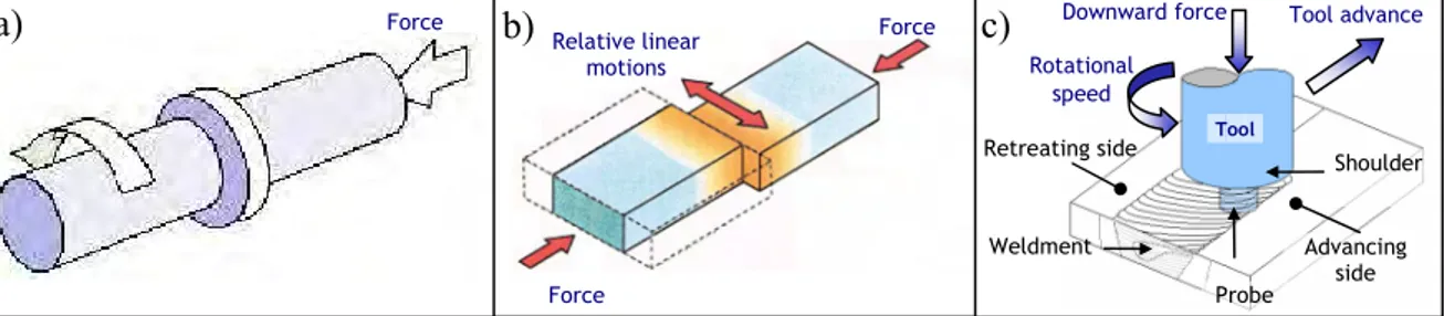
Figure 1: Friction welding processes: a) Rotary Friction Welding, b) Linear Friction Welding, c)

Friction Stir Welding. 15

-Figure 2: Friction Stir Welding phases: a) Initial state b) the plunge, c) dwelling phase, d) welding

phase 16

-Figure 3: Illustration of the different microstructural regions in a transverse cross section of the

weldment 18

-Figure 4: Illustration of the Friction Stir Welding phase 19

-Figure 5: Illustration of two different tool shapes. 19

-Figure 7: Longitudinal (leftside) and transverse (rightside) prints of the temperature field

calculated with the analytical model of Gould and Feng [1]. 23 -Figure 8: Stresses observed during welding with the FE model of Chen in the three main

directions. 25

-Figure 9: Ulysse’s Eulerian model with coupled thermal computation in tools 26

-Figure 10: Mechanical boundary decomposition of the domain 30

-Figure 11: Example of stress-strain curves for a one-dimensional tensile test 31

-Figure 13: Thermal boundary decomposition of the domain 41

-Figure 14: finite elements for velocity/ pressure and temperature interpolation 44 -Figure 16: Schematic representation of the predictor step in Newton-Raphson iteration 47 -Figure 17: Temperature oscillations due to the thermal shock phenomenon. 51 -Figure 18: Illustration of the specific remapping procedure for nodal variable of rigid tools. 52 -Figure 19: Illustration of the contact condition (where the tool is locally approximated by its

tangent plane πk t

. 54

-Figure 20: Illustration of the contact loss for a simple 2D convex angle. 57 -Figure 21: Illustration of the “flip-flop” effect for a simple 2D concave angle. 59 -Figure 22: First case, the contact surface and the transformed contact surface. 60 -Figure 23: Second case, the contact surface consists in two planes. 60

-Figure 24: Smoothing of the contact surface. 61

-Figure 25: Third case of a convex angle. 62

-Figure 26: Smoothing of the contact surface in the convex case. 62

-Figure 27: Limit of the contact surface transformation. 63

-Figure 28: Facets of CCCCA in actual 3D for a surface discretization with triangles. 64

-Figure 29: Definition of the θθθθB angle. 65

-Figure 30: Indentation of a cube with a pyramid. 67

-Figure 31: Indentation of a cube with a facetized cylinder. 68

-Figure 32: Indentation of a cube by a tool that combines concave and convex facets (on top). Indentation of the complementary surface of the same previous tool design with

symmetry plan on 2 lateral faces. 69

-Figure 33: Simulation of the orthogonal cutting process. The smoothing procedure is utilized to

introduce the cutting radius of the tool. Visualization of the equivalent strain rate. 70 -Figure 34: schematic representation of an updated Lagrangian description. 72

-Figure 35: schematic representation of a Eulerian description. 72

-Figure 36: schematic representation of an Arbitrary Lagrangian Eulerian description. 73 -Figure 37: Geometrical splitting method : projection on B-Spline surface 80 -Figure 38: Schematic representation of instabilities generated by tangential movements of the

surface. 81

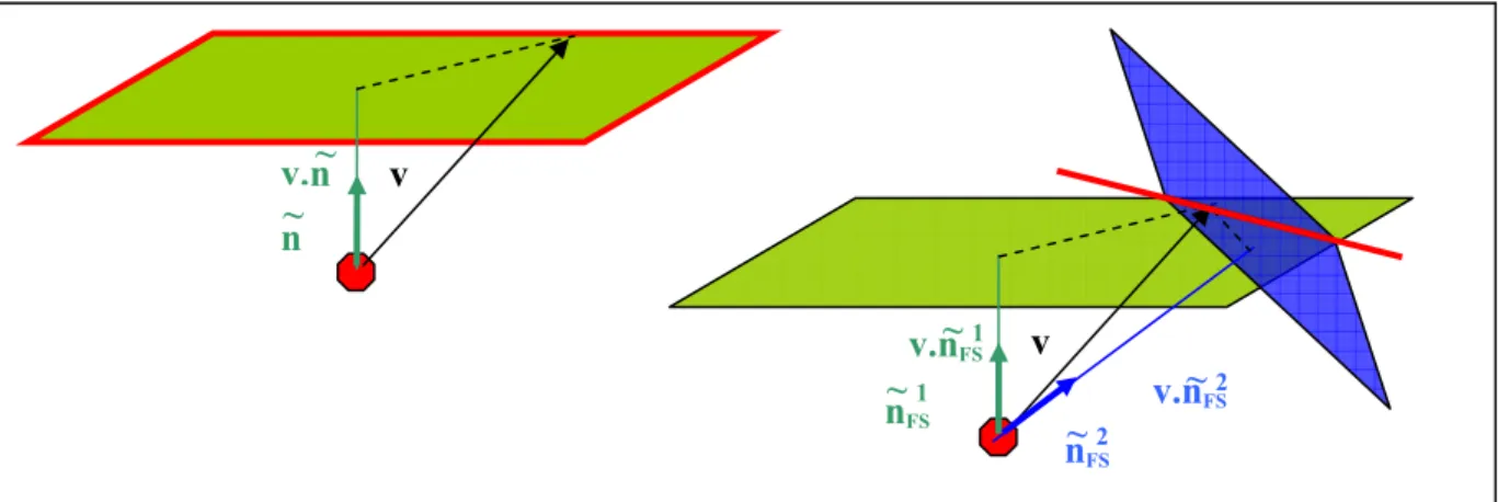
-Figure 39: Graphic representation of possible locations of a node after the imposition of the

contition (IV-18) for one or two normals 82

-Figure 40: Nodal patch Γm 83

-Figure 41: 2D schematic representation of the additional projection procedure for grid velocity

computation 85

-Figure 42: Free surface during an ALE welding simulation: without the projection procedure (on

(12)

-Figure 43: Critical zones of tangential movement of the contact limiting nodes for welding

simulation. 87

-Figure 44: Motivation for adding penalizing free-surface normal for a node already in contact. 88

-Figure 45: Possible folding zones during welding simulation 89

-Figure 46: Shematic representation of folds treatment. 89

-Figure 47: 2D illustration of the mesh velocity averaging 90

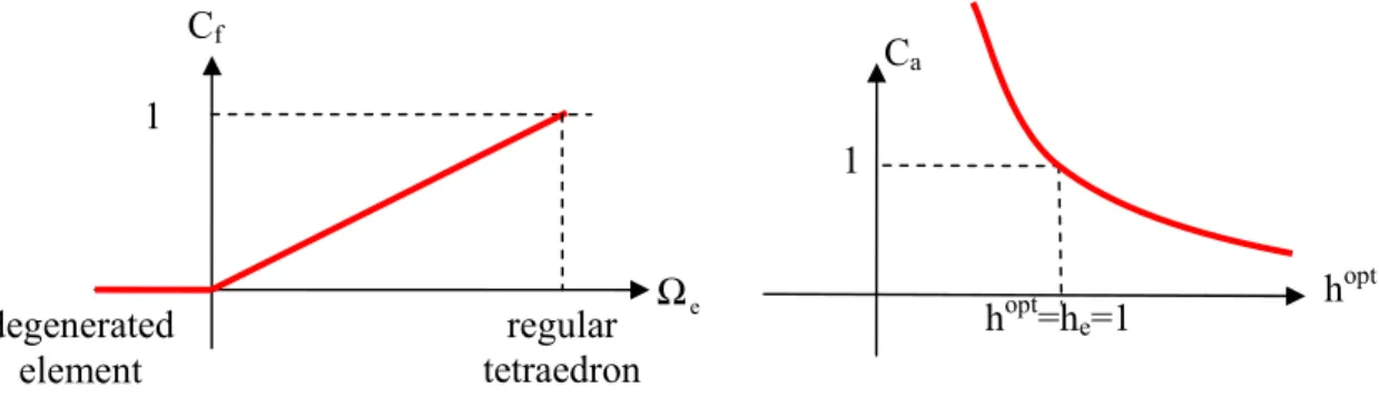
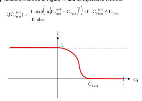
-Figure 48: curves of the geometrical form coefficient and the adaptive coefficient for a given

element size he=1 97

-Figure 49: ξ function curve for combination of the geometrical form coefficient and the adaptive

coefficient. 98

-Figure 50: Schematic representation of the first step of the iterative initializing procedure 99 -Figure 51: Schematic representation of the second step of the straightening procedure 100 -Figure 52: illustration of huge displacements generated by little size modifications. 102

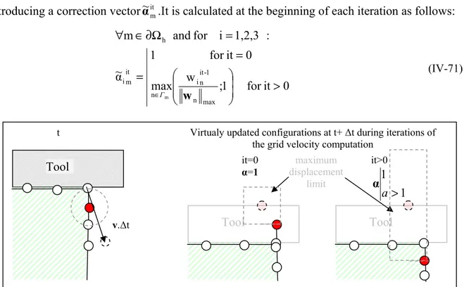
-Figure 53: Maximal velocity allowed on surface patch Γm 102

-Figure 54: schematic representation of the limited grid displacement in a problematic case which

shows the interest of the coefficient α 103

-Figure 55: Schematic representation of the complete developed algorithm to compute the grid

velocity 105

-Figure 56: Classical P1 interpolation technique 107

-Figure 57: Upwind element 109

-Figure 58: P0 remapping 110

-Figure 59: P0 particle remapping 111

-Figure 60: P0 averaging technique 112

-Figure 61: P0 averaging technique 113

-Figure 62: Patch centred on an element in 2D 116

-Figure 63: Patch centred on an element in 2D 116

-Figure 64: 2D illustration of non sufficient number of neighbours 118 -Figure 65: 2D illustration of the addition of points in minimal patches of boundary elements 119 -Figure 66: Method proposed by Srikanth et al. to ensure the respect of equilibrium after

r-adaptation. 120

-Figure 67: Patch for PR2E and REP2 techniques (schematized in 2D) 122 -Figure 68: Schematization of the differences between the developed methods. 125 -Figure 69: Nodal extrapolation technique for P0 variable remapping (schematized in 2D) 127

-Figure 70: Patch centred on a node in 2D 129

-Figure 71: Patch centred on a node in 2D, with nodal values to recover. 130 -Figure 72: Schematization of the nodal recovery techniques for P0 variables remapping. 131

-Figure 73: Sub-tetrahedron interpolation 133

-Figure 74: Construction of the constant field to remap on the grid A 134 -Figure 75: Two mesh refinements utilized for testing the remapping efficiency 134 -Figure 76: Comparison between Nodal Upwind technique and Classical P1 Interpolation technique

for nodal variable remapping 136

-Figure 77: Results obtained with the PR2 technique for nodal variable remapping with two

different grid refinements. 137

-Figure 78: Comparison between the P0 and PR1 techniques for an element variable remapping. 138 -Figure 79: Comparison between the Nodal Least Square Classical smoothing technique and SPR

technique for an element variable remapping. 139

-Figure 80: Results obtained with the PR2 technique for element variable remapping with two

different grid refinements. 140

-Figure 81: Holed plate for the benchmark test 141

-Figure 82: Four gauss points remapping for global error computation 142

-Figure 86: Test dimension. 146

-Figure 87: Scheme of the studied process: orthogonal cutting at high speed 146 -Figure 88: Coupled with smoothing tool procedure, the adaptive ALE formulation handles

problems of mesh distortions in the contact area while complex free-surfaces of the

segmented chip. 146

(13)

-Figure 94: A view of the experimental clamping system, with the cooling plate. 151 -Figure 95: Cooled tool holder and electronic indicator used to measure shoulder depth. 152 -Figure 96: Typical data provided by the experimental equipment during one welding run. 155 -Figure 97: Photos of some experimental welding runs, and some tool utilized to study the pin

length influence. 156

-Figure 98: Global view of the tool and mesh visualisation. 158

-Figure 99: Global view of the body modelisation and initial temperature field (resulting from a

preliminary plunge simulation). 160

-Figure 100: Table of coefficients of the Hansel-Spittel constitutive laws of Al 6061; equivalent stress versus temperature and strain rate for hot and cold constitutive laws (at different

strain rates / temperatures). 162

-Figure 101: Yield stress visualization for the tabulated values of the material consistency K and its

strain rate sensitivity m. 163

-Figure 102: Thermal characteristics of the modelled materials 163

-Figure 103: Thermal boundary conditions of the model 164

-Figure 104: Experimental data recorded for one experimental weld test. 165 -Figure 105: Comparison of forces and torque recorded for two experimental runs processed with

the “same” parameters (experimental dispersion). 166

-Figure 106: Illustration of the global temperature map obtained at steady state (after 60s of

welding). 166

-Figure 108: Comparison of simulated forces, for three different couples of friction parameters,

with experimental data. 168

-Figure 109: Approximate losses of the FSW machinery at various spindle speed levels. 169 -Figure 110: Comparison of simulated torques for three different couples of friction parameters,

with experimental data 170

-Figure 111: Comparison of simulated temperatures with experimental measurements, for the three

couples of friction parameters. 171

-Figure 112: Comparison of simulated forces for two different welding speeds and with

experimental data 172

-Figure 113: Comparison of simulated forces for two different welding speeds and with

experimental data 173

-Figure 114: Movement of Lagrangian particles when passing through the welding tool at steady

state. 173

-Figure 115: Movement of Lagrangian particles when passing through the welding tool at steady

state. 174

-Figure 116: A view of the experimental plunge, just prior to the test. Notice the thermocouple wires

extending out from the bottom of the block. 175

-Figure 117: A drawing of the FSW tool and plate geometry used in the experimental plunge test, all dimensions in millimeters. Notice the holes placed in the material to allow for the

insertion of thermocouples. 177

-Figure 118: Global view of the model with numerical sensors located as in the experimental

plunging test 178

-Figure 119: Yield Stress visualization for hot and cold constitutive law for Al 7075 180 -Figure 120: Temperature map in the cutting joint plane during the plunging phase. * viscoplastic

friction is use with αf=0.4 and p=0.125 * the tool is untilted and unthreaded 182

-Figure 121: Averaged temperature experimentally measured into tool during the three plunging

experiment. 183

-Figure 123: Plots of temperature histories in the plate during the experimental 6 seconds plunge at

various radii from the pin center. 184

-Figure 124: Temperature at Eulerian sensors located in the workpiece during the plunge

simulation. 185

-Figure 125: Cross section of a 7075 sample after plunging, showing mechanically and thermally

areas and thermocouple locations. 186

-Figure 126: Comparison between the simulated temperature field and microstructure observation

(14)

-Figure 127: Comparison between the experimentally observed MAZ and simulated equivalent strain field in the cross section when the shoulder is just getting in contact with the

plate (t=5.4 s) 187

-Figure 128: Axial force (top graph.) and Motor Power (bottom graph.) registered during the

experimental plunging test. 188

-Figure 129: z- force and equivalent motor power simulated during the plunging phase 189 -Figure 132: Temperature histories calculated with Forge3 at the six thermocouple locations. 191 -Figure 133: Comparison of the experimental z-force with the force preliminary simulated using the

initial Lagrangian formulation of forge3 192

-Figure 134: Visualization of the material flow using Lagrangian sensors during the plunge

simulation. 193

-Figure 135: Comparison of vertical forces and torques observed for the dwelling phase simulation

with (on right) and without (on left) low plunge velocity. 195 -Figure 136: Comparison of the temperature field observed after 2.5 s of dwelling phase simulation

with (bottom) and without (on top) low plunge velocity. 195 -Figure 138: Temperature field during transient states of the whole process (cross section view): a)

initial state, b-c) plunging phase, d) end of the plunging phase, e) after dwelling phase,

f) transient welding phase. 198

-Figure 139: Visualization of the temperature field obtained after 13s of welding with ALE formulation in the cutting joint plan (on left side) and top view of the friction area at

the same time (on right side): blue nodes are not in contact. 200 -Figure 140: Comparison of resulting forces between the Eulerian and ALE simulations. 200 -Figure 141: Fold appearance at the end of the plunging phase simulation with a tilted tool (cross

section view) 201

-Figure 142: Experimental flash formation during welding (top view and transverse cross section). 202 -Figure 143: Example of flash occuring during an ALE simulation of transient welding phase. 203 -Figure 144: Initial void formation due to bad initial state (cross section view) The void tends to be

field but leads to material interpenetration which is not handled by the code. 204 -Figure 145: Illustration of the additional virtual axial velocity for modelling the influence of the

threads. 205

-Figure 146: Comparison of temperature maps in the cross section during the plunging phase for viscoplastic friction at top (αf=0.4 and p=0.125) and Coulomb limited Tresca in the

middle (µ=0.5) and screwded pin (2mm equivalent pitch) at the bottom. 206 -Figure 147:Comparison of temperatures recorded at three locations in tool during a 7s plunge in

cases of unthreaded tool, 2mm and 10mm equivalent screw pitch (Norton friction is

used with αf=0.4 and p=0.125). 207

-Figure 148: Comparison of temperatures recorded at three locations in the tool during a 7s plunge in cases of Norton friction law (with αf=0.4 and p=0.125) and Coulomb friction law

(µ=0.5) (pin is unthreaded). 208

-Figure 149: Comparison of temperature values during the plunge phase simulation at sensors

located at 20.6 and 12.7 mm from the tool axis in the three different studied cases. 208 -Figure 150: Comparison of torques and axial forces during the plunge phase for the three studied

cases: viscoplastic friction law (αf=0.4 and p=0.125), Coulomb friction law (µ=0.5) and

threaded pin (10mm equivalent pitch). 209

-Figure 151: Comparison of the equivalent strain maps in the cross section after a 7 s plunge for

unthreaded pin on right and threaded pin on left (10 mm equivalent pitch). 209 -Figure 152: Comparison of the ALE welding phase with threaded and unthreaded pin tool. At top,

temperature after 21s of welding (cross joint section view) At bottom, equivalent

strain at the back of the pin. * Viscoplastic friction is use with αf=0.4 and p=0.125 211

-Figure 153: Comparison of stream lines simulated with and without threads. 212 -Figure 154: Comparison of Forces and equivalent Motor Power for threaded and unthreaded tool

resulting from experimental and numerical simulation 213

-Figure 155: Illustration of the modified additional virtual velocity for modelling the influence of

(15)

-Figure 156: Temperature map (cross section view) after 12 s of an ALE welding simulation. The contact is lost for some of the nodes at the bottom trailing side of the pin while the

action of threads is simulated through a 10 mm equivalent screw pitch. 214 -Figure 157: Comparison of experimental transverse cut and simulated equivalent strain in a

transverse cutting plane at the back of the pin. 214

-Figure 158: New tool shape: experimental tool (on top right) and modelled one (The arrows

illustrate the added virtual velocities for threads modelling). 216 -Figure 159: “foot print” (contact area) comparison. At t=0 at the top left, after 2 s with the

unthreaded tool at the top right, and after 17 s of welding simulation with the

threaded tool at the bottom (blue nodes are not in contact with the tool). 217 -Figure 160: Interesting results with new tool design: Equivalent strain in transverse cross section

at the back of the probe on the left and material stream lines computed after 17 s of

welding simulation on right 218

-Figure 161: Temperature map in the cross joint section: initial state (a-priori built) and after 17s of

(16)

-Introduction: The FSW Process

Chapter I :

Introduction: The FSW process

1 Process description

1.1 Friction welding processes: advantages and potential uses

Friction Welding (FW) converts mechanical energy into heat and material deformation to create a weld. Currently, the parent material is not melt. Joining occurs in the solid state, avoiding possible metallurgical complications such as porosity, cracking or detrimental metallurgical changes.

One of the main advantages of the friction-based technologies is that thus enable joining material combinations which were previously difficult to weld. Furthermore, compared to traditional arc welding, FW produces little or no weld distortion, porosity or fume, and has excellent mechanical properties.

Rotary friction welding (Figure 1a) has been used for about fifty years in industry and is still the most widely used of the friction welding technologies. Non-rotary welding (linear, orbital and angular reciprocating motions -Figure 1b) has been a first major extension. It permits the joining of noncircular shapes such as squares and rectangular bars, which are very difficult to weld with rotary technology providing correct alignment. But the Friction Stir Welding (FSW) process has enlarged the application field of friction-based technologies since its invention in 1991 at The Welding Institute in England (Figure 1c).

Figure 1: Friction welding processes: a) Rotary Friction Welding, b) Linear Friction Welding, c) Friction Stir Welding.

FSW has been successful in welding a wide range of materials such as plastics, metal matrix composites, aluminium, copper, steel, stainless steel, nickel alloys, and titanium. FSW Downward force Tool advance Rotational speed Weldment Probe Retreating side Advancing side Shoulder Tool Force Force Relative linear motions a) Force b) c)

(17)

has already been successfully implemented in various applications involving aluminium and copper in many industries including marine, aerospace, and railways.

The evolution of FSW equipment over the last decade has expended the potential of this innovative manufacturing technology and new developments in process application, such as underwater FSW of steel or stainless linepipes, have been proposed. The machines, which were originally converted milling machines, are currently designed with force control in mind. Improvements in the wear resistance, fracture toughness, and design of FSW tools continue to enhance the feasibility of FSW in a large variety of materials.

This recent friction stir technology can also be exploited to consolidate or refine the microstructure of a material. This kind of use also involves application of friction and pressure but as it does not imply creation of bond between two pieces of material, it is called Friction Stir Process (FSP).

In this manuscript we shall abusively use the abbreviations FSP or FSW without any distinction. The numerical modelisation of the FSW process does not take into account the interface between the two pieces of material to weld: therefore the simulation is basically equivalent to FSP simulation. The experimental weldings discussed and compared to numerical simulations in the last part of this manuscript have also been performed on a single plate.

1.2 Friction Stir Welding Process

The FSW process combines frictional heating and stirring motion to soften and mix the interface between two workpieces, yielding a solid, fully consolidated weldt.

(18)

Introduction: The FSW Process

First, parts are mated together, rigidly clamped (Figure 2a). A rigid cylindrical spinning tool, composed by a protruding pin and a larger concentric shoulder, is plunged into the joint line until the shoulder rests on the surface: this is the plunging phase (Figure 2b). The dwelling phase (Figure 2c) follows and rapidly softens the material through frictional heating. Then the tool is advanced along the joint line: the material is plastically deformed, stirred around the tool pin in a complex movement depending on forces involved and tool design (Figure 2d). This welding phase provides a solid, fully consolidated weldment between the matted parts.

Temperatures in the tool and workpiece are often close to the solidus temperature of the workpiece (3-8 kW of mechanical power are converted into heat during each weld of aluminium alloys). A complete understanding of the FSW process through thermo-mechanical simulation requires carefully considering both workpiece and tool.

The thermo-mechanical process involved under the tool results in different microstructural regions (see Figure 3). Some are common to all forms of welding, others are unique to the technique.

The stir zone (also called nugget, the dynamically recrystallised zone) is a region of heavily deformed material that roughly corresponds to the location of the pin during welding. The grains within the stir zone are roughly equiaxed and often an order of magnitude smaller than the grains in the parent material. A unique feature of the stir zone is the common occurrence of several concentric rings, which has been referred to as an ‘onion-ring’ structure. The precise origin of these rings has not been firmly established, although variations in particle number density, grain size and texture have all been suggested.

The flow arm is on the upper surface of the weld and consists of material that is dragged by the shoulder from the retreating side of the weld, around the rear of the tool, and deposited on the advancing side.

The thermo-mechanically affected zone (TMAZ) occurs on either side of the stir zone. In this region, the strain and temperature are lower and the effect of welding on the microstructure is correspondingly smaller. Unlike in the stir zone, the microstructure is recognizably that of the parent material, albeit significantly deformed and rotated. Although the term TMAZ technically refers to the entire deformed region, it is often used to describe any region not already covered by the terms stir zone and flow arm.

(19)

The 'heat affected zone' (HAZ) is common to all welding processes. As indicated by the name, this region is subjected to a thermal cycle but is not deformed during welding. The temperatures are lower than those in the TMAZ but may still have a significant effect if the microstructure is thermally unstable. In fact, in age-hardened aluminium alloys this region commonly exhibits the poorest mechanical properties.

Figure 3 : Illustration of the different microstructural regions in a transverse cross section of the weldment

1.2.1.1 Process parameters

For FSW (Figure 4), two parameters are very important: tool rotation rate (ω, rpm) in clockwise or counterclockwise direction and tool traverse speed (v, mm/min) along the line of joint. Rotation of the tool results in stirring and mixing of material around the rotating pin, and the translation of tool moves the stirred material from the front to the back of the pin, and finishes the welding process. Higher tool rotation rates generate higher temperature because of higher friction heating, and result in more intense stirring and mixing of material. However, it should be noted that friction between tool and workpiece governs the heating, and that the coefficient of friction at the interface will change with increasing tool rotation rate. So, a monotonic increase in heating with increasing tool rotation rate is not expected.

Nugget zone thermo-mechanically affected zone (TMAZ)

Heat-affected zone (HAZ)

(20)

Figure 4 : Illustration of the Friction Stir Welding phase

In addition to the tool rotation rate and traverse speed, another important process parameter is the insertion depth of the pin into the workpiece (also called target depth). This parameter is related to the pin length. When it is not enough, the tool shoulder does not correctly contact the original workpiece surface. Thus, it cannot move the stirred material efficiently from the front to the back of the pin, resulting in generation of welds with inner channels or surface grooves. When the insertion depth is too deep, the tool shoulder plunges into the workpiece creating excessive flashes. In this case, a concave weld is produced, with a local thinning of the plates in the welded zone.

Further, the angle of the spindle, or tool tilt, with respect to the workpiece surface is important for producing sound welds with smooth tool shoulders. A suitable tilt of the spindle towards trailing direction ensures that the shoulder of the tool holds the stirred material by the threaded pin and moves material efficiently from the front to the back of the pin. It should be noted that the recent development of ‘scrolled’ tool shoulder allows FSW without tool tilt (see illustration in Figure 5). Such tools are particularly preferred for curved joints.

Figure 5 : Illustration of two different tool shapes. Downward force

Tool advance speed v Rotational speed ω Joint _Probe Retreating side Advancing side Shoulder Joint line Tool Tilt angle Concave shoulder Threaded pin Scrolled convex tool shoulder Scrolled conical pin

(21)

1.2.1.2 Tool geometry

Tool geometry is the most influential aspect of process development. The tool geometry plays a critical role in material flow and consequently governs the traverse rate at which FSW can be conducted. As mentioned earlier, the FSW tool has two primary functions: to produce a localized heating and a material flow.

In the initial stage of the tool plunge, the heating mainly results from the friction between the pin and the workpiece. Additional heat is produced by the deformation of the material. The tool is plunged till the shoulder touches the workpiece. The friction between the shoulder and workpiece results in the largest component of heating. From the heating standpoint, the relative size of pin and shoulder is the most important, and the other design features are not critical. The shoulder also provides confinement for the heated volume of material.

The second function of the tool is to ‘stir’ and ‘move’ the material. The uniformity of microstructure and properties, as well as process loads, are governed by the tool design. At present, concave shoulder and threaded cylindrical pin are generally used.

With increasing experience and some improvements in understanding the material flow, the tool geometry has evolved significantly. New complex design features are regarded to (a) reduce welding force, (b) enable easier flow of plasticized material, (c) facilitate the downward augering effect, and (d) increase the interface between the pin and the plasticized material, thereby increasing heat generation.

The tool geometry has a significant effect on the metal flow. The correlations between the material flow and the resultant microstructure of welds varies with each tool design. The generalization of microstructural development and influence of processing parameters is difficult in absence of the tool information. Therefore, a critical need is to develop a systematic framework for tool design. In friction stir welding conferences, several companies have indicated internal R&D efforts but no open literature is available on such efforts and outcomes.

Computational tools, including finite element analysis (FEA), can be used to visualize the material flow and calculate axial forces. However any generalization should be treated carefully because the material flow is very significantly influenced by the tool design, while

(22)

most studies do not report the utilized tool design and all process conditions. Therefore, the differences observed between various studies cannot be easily compared.

1.2.1.3 Microstructure and texture

The solid-state nature of FSW, combined with its unusual tool and asymmetric features, result in a highly characteristic microstructure. Some regions are common to all kinds of welds but some are quite unique to the technique.

Texture influences a variety of properties, including strength, ductility, formability and corrosion resistance. As mentioned earlier, the FSW material consists of distinct microstructural zones (see Figure 6), i.e., nugget, TMAZ, HAZ and base material. Each zone has a different thermo-mechanical history. What is even more complicated in FSW is that the nugget zone consists of several sub-domains. For example, the top layer undergoes a specific deformation by the shoulder after the pin has passed through it. On the other hand, depending on the tool rotation rate and traverse speed, the nugget region can have an onion ring pattern or other microstructural alterations. In the last decade, the use of orientation imaging microscopy (OIM) has shown to be a very valuable tool, not only for obtaining the texture information, but also for establishing the grain boundary misorientation distribution from same set of experiments.

1.2.1.4 Residual stresses

During fusion welding, complex thermal and mechanical stresses develop in the weld and the surrounding region due to the localized application of heat and resulting constraint. The residual stresses usually reach the yield strength value of the base material. On the other hand, it is generally considered that residual stresses are much lower in friction stir welds due to much lower temperatures. However, compared to rather compliant clamps used for fixing the parts in conventional welding, the very rigid clamping used in FSW exerts a much higher restraint on the welded plates. These restraints impede the contraction of the weld nugget and heat-affected zone during cooling in both longitudinal and transverse directions, thereby resulting in generation of longitudinal and transverse stresses. High values of residual stresses

Figure 6: Example of microstructure observed in TMAZ and HAZ

(23)

have a significant effect on the postweld mechanical properties, particularly the fatigue ones. Therefore, it is of practical importance to carefully investigate the residual stress distribution in the FSW welds.

2 Motivation and problem statement

2.1 Motivation and numerical objectives

FSW is still a recent and complex process. Sound welds are achieved only for specific combinations of the process parameters. The particular phenomena, which are responsible of the deposition of material that occurs at the trailing edge of the probe, are not completely understood yet. Many experimental investigations have already been conducted to adjust input parameters (spindle speed, feed rate, and tool depth), contrary to numerical investigations, which have been scarcely used for these issues.

Firstly computational tools could be helpful to better understand and observe the influence of input parameters on resulting phenomena. Visualization and analysis of the material flow, temperature map, stresses and strains involved during the process is much easier in simulations than in experiments.

Moreover, the process results in significant microstructural evolution, including grain size, grain boundary character, dissolution and coarsening of precipitates, break-up and redistribution of dispersoids, and texture. The numerical modelisation can provide mechanical and thermal histories of material particles, which are necessary to compute final microstructure of the weld. Thus the numerical tool can also be helpful for understanding and controlling the final microstructure and properties of welds.

Therefore and secondly, predictive simulations could help to adjust and optimize the process parameters and tool designs in order to achieve the best weld properties, increase welding rates and tool life, and enlarge the application field of the process by reducing stresses on FSW tool.

The main objective of this work is to develop a 3D robust numerical tool enabling the thermo-mechanical simulation of the whole FSP (plunging phase, dwelling phase and welding phase). As numerical simulation has to be as predictive as possible, the accuracy of the developed methods is crucial.

(24)

2.2 Difficulties and background literature

FSW results in intense plastic deformation and temperature increase within and around the stirred zone. It induces complex movement of material, large shear forces in the plastically deformed material, raising the temperature of the material to about 80% of the melting temperature [1]. Therefore, this process is highly thermo-mechanically coupled and presents a formidable challenge for researchers attempting to characterize these phenomena through various modelling techniques.

First models reported in the literature for FSW were analytical models addressing temperature analysis. Initially based on Rosenthal’s equations, they describe the quasi-steady temperature field of a semi-infinite body on which is applied a surface heat source moving with constant velocity. The heat source really produced around the tool is replaced by simple analytical solutions [2]. McClure et al.[3], along with Gould and Feng [4] have incorporated in their equations the term of frictional heat assuming a constant uniform pressure between the tool and the part. Figure 7 shows the temperature field described by the analytical model of Gould and Feng. The traverse speed of the tool, as the rotational velocity ω and the loading force F are the three parameters of the model.

Figure 7: Longitudinal (leftside) and transverse (rightside) prints of the temperature field calculated with the analytical model of Gould and Feng [1].

An expression of the estimated analytical heat generation, developed by Schmidt et al

[5]for more complex tool shapesis the following:

z

x

z

y

F

v

ω

(25)

(

)

(

)

(

probe

)

2 probe 3 probe 3 probe 3 shoulder 2 shoulder exp ana , sliding R R 1 tanα R 3R H R F µω 3 2 Q = − + + + (I-1)

Rprobe and Rshoulder are respectively the radius of the probe and the shoulder of the tool. The pin

length is given by Hprobe. Fexp is the plunge force experimentally observed. µ is the Coulomb

friction coefficient. α is the cone angle of the tool shape. Thereafter, the convective heat transfer due to the material flow in the shear layer have been taken into account (using sticking conditions in a simplified way) by prescribing a velocity boundary condition for the convective term in the energy equation. Kandkar et al [6]introduced a torque based heat input model in which the local heat flux q& is linearly related to the distance to the tool axis r as follows: ω P with H R 2π R π 3 2 .ω . (r) q av tot probe 2 probe 3 shoulder tot = + = rM M & (I-2)

Mtot is the total torque and Pav is the average power.

All these models constitute first tools to approximate the temperature map or the heat source in FSW. However, they are based on strong assumptions concerning the contact (sliding or sticking conditions are assumed) and always need the adjustment of experimental coefficients to be predictive. Moreover, these models have low flexibility (tool design and transient phases of the FSP are not taken into account) and they only provide thermal informations. Their major interest is in feeding Finite Element (FE) solid-mechanics models with temperature fields.

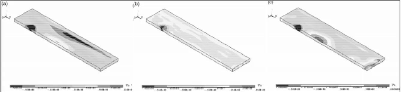
Finite Element (FE) solid-mechanics models have been logically developed after analytical ones. The high distortion of the mesh, when Lagrangian formulation is used, is the main difficulty that Finite Element (FE) solid-mechanics models have to deal with. They occur under the tool shoulder, where high strains are logically observed during FSW. Therefore, the FSW tool is usually substituted by an analytical heat source. This approximation, widely used, allows for compution of residual stresses that are due to thermal distortions. Figure 8 shows the residual stresses provided by the model of Chen and Kovacevic in the code ANSYS [7],

when the heat source is assumed to be symmetric. Lawrjaniec et al. [8] have developed two models using the thermomechanicaly coupled FE codes SYSWELD and MARC. 2D surface heat

(26)

sources or 3D heat sources based on Russel’s equations [9] are assumed taking into account the non-symmetrical character of the process. In WELDSIM, Chao et al. [10] have modelled the

mechanical action of the tool as a uniform forging pressure. A Coulomb friction law is assumed and the frictional heat source due to the rotational movement of the tool is taken into account. But none of these FE solid-mechanics based models enable the material flow simulation.

Figure 8: Stresses observed during welding with the FE model of Chen in the three main directions.

The simulation of material flow during FSW requires robust treatment of large deformations. Thus, at first it has been logically modelled using Computational Fluid Dynamics (CFD) models. Indeed, CFD Software can be easily adapted to FSW process: the material, regarded as a viscous fluid, flows across the Eulerian grid and interacts with the rotating tool. The inlet material velocity prescribed at the boundary of the domain corresponds to the traverse speed of the tool. Figure9 shows the model developed by Ulysse [11]. The contact is assumed sticking and thus, the heat source is only due to the viscous dissipation of the laminar flow [12].Seidel [9] hasapproximated the viscosity by a function of the material yield stress throughout the Zener-Hollomon parameter. Its model has been implemented in the 3D code FLUENT. Colegrove et al. have [13, 14] also used a CFD code to develop a global

thermal model, in which the heat flow (applied at the interface FSW tool/workpiece) includes terms due to material shearing and friction. They have also developed a local model to visualize the influence of the screw on the material flow around the pin.

One of the major drawbacks of these CFD models is the approximation usually resulting on the material rheology, which does not allow for residual stresses prediction. In addition, simulation of transient phases of the process is hardly possible with such Eulerian description of the grid.

(27)

Figure 9: Ulysse’s Eulerian model with coupled thermal computation in tools

Few models have actually taken into account the unilateral contact conditions [15]; they do enforce the contact condition between tool and workpiece, thus prohibiting void formation. The model of Schmidt et al. [16] is currently the only one in literature which handles this condition and so enables simulating under which conditions the material deposition process is successful. It has been developed within the Abaqus Explicit software, and utilizes an Arbitrary Lagrangian Eulerian (ALE) formulation. The remeshing algorithm provides an Eulerian character to the formulation that allows free surface movements to be modeled. The welding speed is prescribed as an inflow velocity at the inlet Eulerian surface which corresponds to the half-circumference of the discretized domain. The plunge phase is not simulated, but a spring force is applied to the tool. It corresponds to the experimental machine stiffness. The initially prescribed plunge depth is automatically provided by the spring back of the tool which settles at a value modelled close to the experimentally found one. The elasticity of the material is modeled by an elastic–plastic Johnson–Cook constitutive equation. The contact is bilateral during the period of time necessary to reach a steady state and unilateral (so enabling void formation) afterwards, in order to verify that the material deposition process correctly occurs. A Coulomb friction law is assumed in this local fully coupled 3D model.

2.2.1.1 Summary

This short bibliographic study highlights several difficulties to simulate FSW. In this process, heat sources result from two different phenomena. In the first hand, heat is generated by friction at the tool/workpiece interface, and in the second hand by energy dissipation during plastic deformation of the material under the tool. The thermo-mechanical coupling is strong

(28)

so the numerical model has to accurately take into account these two terms. The heat source is three dimensional, asymmetrical, and most importantly, dependent of the contact area. Therefore analytical models can only provide a first approximation of the thermal field during the steady phase of the process. The description of the contact area, taking into account the complex tool shape, is crucial.

The thermal boundary conditions are also important to properly model the heat dissipation and the accuracy of the simulation logically requires coupled computations inside the FSW tool and in the backing plate.

The major difficulty of simulating the FSP transient phases consists in dealing with the large deformations, which are involved under the tool, while describing with enough accuracy little surface movements in the contact area. The complex material flow generates large distortions of the mesh when a Lagrangian description is utilized. Thus complex remeshing procedures are required. The Eulerian formulation more easily provides the history of the material flow during stationary welding. Nevertheless, the transient events, such as the phenomenon of filling or of prevailing cavity behind the probe of the tool, are hardly simulated because of the difficulty to track free surface movements.

The ALE description makes it possible to takes into account movements of free surfaces while reducing mesh distortions. This formulation looks procuring the best compromise between advantages and drawbacks of Lagrangian and Eulerian formulations.

Therefore, it seems to be the most adapted description for simulating steady and transient steps of the process. It enables studying one of the less understood aspects of FSW: the condition under which the deposition of material behind the tool is successful. This success depend on an adequate combination of the machining parameters: advancing speed, rotational speed, and depth of the tool inside workpiece. Thus, the model should adequately traduce these parameters in terms of frictional forces and forging pressure.

The keypoint of the present work is developing a robust ALE formulation in the code Forge3 (initially Lagrangian) in order to deal with the different aspects of FSW simulation which have just been presented.

(29)

(30)

Numerical Problem

Chapter II :

Numerical Problem

In the present study, the FORGE3® code has been modified in order to simulate the different phases of FSP. This commercial software is extensively used to simulate hot, warm and cold forging of 3D geometry parts. This solid-mechanics code uses a Lagrangian finite element formulation to solve the thermal and mechanical equations at each time step of the simulated process. These equations are detailed in the first half of this chapter, which also presents global different constitutive equations and boundary conditions used to model the process. The second half is m 4.1ore dedicated to their resolution.

1 Mechanical Equations

The mechanical problem is based on a set of two physical equations, which are numerically integrated.

1.1 Continuity Equation

The continuity equation states that mass cannot be lost or gained in time. This is mathematically expressed in equation (II-1).

0 dt dm

= (II-1)

m is the mass of a given volume Ω. The integration of equation (II-1) gives:

(

ρ(x,t)dV

)

0 dt d dt dm Ω = =

_∫

(II-2)

ρ is the density. Finally, the differentiation of equation (II-2)leads to the continuity equation: 0 v) div(ρ t ρ = + ∂ ∂ (II-3)

If we consider only rigid plastic materials (so neglecting elasticity effects), the time derivative can be considered as null and the incompressibility condition is then written for as:

0 ) (

div v = (II-4)

(31)

0 ) ε

tr(&_pl = _(II-5)

1.2 Motion Equation

The general form of the motion equation is expressed in equation (II-6) as a force balance, including dynamic forces (inertia), static forces, and gravity.

g σ div

γ ( ) ρ.

ρ. = + (II-6)

γ is the acceleration, g is the gravity acceleration and σ the stress tensor of Cauchy. Gravity and inertia are often neglected in most static force problems.

1.3 Boundary conditions

The boundary of the mechanical domain Ω is called ∂Ω. It can be divided into several distinct boundary conditions resulting in the definition (II-7) (see Figure 10).

T V L C Ω Ω Ω Ω Ω=∂ +∂ +∂ +∂ ∂ (II-7)

Figure 10: Mechanical boundary decomposition of the domain

• On ∂ΩL, the free surface conditions impose that the normal stress is null:

0 n

σ. = (II-8)

where n is the normal out warding the surface.

• On ∂ΩT , imposed loading conditions force to have equation (II-9).

T

σ.n= (II-9)

• On ∂ΩV, the velocity is imposed, so we have equation :

T : Imposed load Tool

Ω

∂∂∂∂

Ω

L ∂∂∂∂

Ω

_T ∂∂∂∂

Ω

_V ∂∂∂∂

Ω

_C V0: Imposed velocity v vtool n

(32)

Numerical Problem

0

v

v= (II-10)

• On ∂ΩC, two kinds of conditions are imposed due to contact:

- a non penetration condition in the normal direction, given by the Signorini equations:

[

( )

]

σ 0 0 σ 0 . ) ( n tool n tool = − ≤ ≤ − .n v v n v v (II-11)

vtool is the displacement of the tool; σn =(σ. )n .n is the contact pressure.

Note: The notation . is used both for matrix or scalar products.

- and a friction condition in the tangential direction, imposing the boundary shear stress τf:

n n σ

τf = . −σn. (II-12)

τf depends on the friction equations introduced in paragraph 2.2.

2 Modelling the problem

2.1 Constitutive models

2.1.1 Definitions

Figure 11: Example of stress-strain curves for a one-dimensional tensile test

The constitutive equations define the relation between stress σσσσ and strain εεεε. It is generally based on experimental observations. The type of employed constitutive model depends on the

ε σ εel εpl σy,0 ε > ε0 . . ε = ε0 . .

(33)

material under investigation, and the applied loads. It is also possible that the behaviour depends on the strain rate ε& (see Figure 11) and the temperature T. A general expression is given by the following equation:

(

ε,ε,T,P

)

σ

σ= & (II-13)

P is a set of coefficients called rheological parameters which are used in the constitutive equation.

The stress tensor is split into a deviatoric part s, called deviatoric stress, and a spherical one pI, as follows:

I s

σ= −p (II-14)

The hydrostatic pressure p is defined by the equation (II-15). )

tr( 3 1

p=− σ (II-15)

The strain rate tensor is defined as:

(

)

2

1 _∇ ₊ _∇

= .v v.

ε& (II-16)

One-dimensional representation of stress, and strain rate are respectively given by the equivalent Von Mises Stress tensor (equation 17)) and the equivalent strain rate (equation (II-18)).

The equivalent strain is defined by the time integration of the equivalent strain rate:

∫

= t 0 dt ε ε & (II-19)

For hot processes, the elastic strain is often neglected and the behaviour of the metal is often modelled by a viscoplastic constitutive law. On the other hand, elastic strain can not be neglected in cold processes, therefore elastoplastic, elasto-viscoplastic, or pure elastic laws can be considered. s s : 2 3 σ = (II-17) ε ε && & _: 3 2 ε = (II-18)

(34)

Numerical Problem

A strong gradient of temperature takes place in FSW process. The material is highly softened under the tool and has a viscoplastic behaviour in this area. Nevertheless, an elasto-viscoplastic constitutive law has to be considered in order to accurately simulate the plunging phase and the global matrix response in the far-field. This latter is crucial to observe loading effects and compute residual stresses, which appear during the cooling of the workpiece.

An additive Prantl-Reuss decomposition of the strain rate into elastic and plastic parts is assumed (equation (II-20) and Figure 11).

2.1.2 Elasticity

Elasticity characterizes a reversible linear behaviour. The Hooke’s law (equation (II-21)) is representative of a linear elastic and isotropic material rheology. Its time derivative is given as:

( )

(

)

(

1 ν

)(

1 2ν

)

ν E λ et ν 1 2 E µ λ µ 2 el el el − + = + = + = =Dε ε trε

σ& & & &

(II-21)

λ and µ are the Lamé coefficients, which are constant for homogenous material (and linearly time dependent). E is the Young modulus, ν is the Poisson coefficient, ε& is the elastic el strain rate and σ& is the time derivative of stress.

The inverse form of this Hooke law is written as follows:

( )

σ I σ

σ D

ε& & & tr & E ν E ν 1 1 -el ₌ ₌ + ₋ (II-22) 2.1.3 Elastoplasticity

Elastoplasticity correctly models the rheology of metal in cold forming processes. As illustrated in Figure 11, the yield stress σy is defined as the minimal stress to create a plastic

non-reversible strain in a given direction. A basic goal of phenomenological plasticity models is to replicate the one-dimensional tension test. To achieve this, a scalar function has to be defined as plasticity criterion:

( )

,σ 0 plasticbehaviour f behaviour elastic pure 0 σ , f y y ⇒ = ⇒ < σ σ (II-23) pl el ε ε

(35)

The Von Mises criterion is commonly used for modelling isotropic metals. It is expressed in the principal stresses referential as follows:

(

) (

)

2 y 2 II I 2 III II 2 II I σ σ σ σ σ 2σ σ f = − + − + − − (II-24)

Using the splitting formulation (II-14) of the stress, (II-24) becomes:

(

)

2 y 2 III 2 II 2 I s s 2σ s 3 f = + + − (II-25)

Note that the plastic flow occurs when: s : s s = =tr( ) σ 3 2 2 2 y (II-26)

So, using the equivalent Von Mises stress tensor definition of equation (II-17), the plasticity criterion can be finally written in the simple form:

y y) 0 σ σ

σ ,

f(σ = ⇔ = (II-27)

Because the six-dimensional stress space is collapsed into a single number, many stress states may produce the same equivalent stress (they collectively define a surface in stress space). The particular collections of stress states that satisfy equation (II-27) define the yield surface. The plastic strain rate is assumed parallel to the normal of the yield surface. The intensity Λpl of the plastic strain rate obeys the flowing rule:

Λpl

is a proportional constant that must be determined to complete the plasticity model.

Λpl

is always greater than, or equal to zero, because a negative value would imply that the response is elastic.

So for a Von Mises criterion, the equation (II-28) becomes:

y pl pl σ 2 3 Λ s ε& = _(II-29)

And because of the incompressibility of the plastic strain, we have: 0

)

tr(ε&pl = (II-30)

So for a plastic material, the stress deviator is given by:

pl pl y ε 3 2 & &ε s= σ (II-31) σ ε ∂ ∂ Λ = pl f pl & (II-28)

(36)

Numerical Problem

The evolution of the yield stress σy may be described through a function of the equivalent

strain, the temperature, the pressure…

) , , ( T p y y σ ε σ = (II-32)

To resume, the equations of elastoplasticity are:

( )

        =∂ ∂ Λ = = + = − 0 σ , D y pl pl 1 el pl el σ σ ε σ ε ε ε ε f f & & & & & & (II-33) 2.1.4 Viscoplasticity

The elastic component can legitimately be neglected when modelling material flows at hot temperatures, and a viscoplastic potential ϕ can be highlighted. This latter connects the stress deviator s to the plastic strain rate ε& :

ε s & ∂ ∂ = ϕ (II-34)

In the Forge3® software, the Norton-Hoff viscoplastic potential can be used:

( )

m 1 ε 3 1 m k + + = & ϕ (II-35)

k is the consistency of the material; m is the sensitivity to strain rate and highlights the difference between plastic and viscoplastic behaviour.

The Norton-Hoff constitutive law is deduced from (II-18), (II-34), (II-35) :

( )

ε ε

s=2K 3ε& m−1&=µ(ε&) & (II-36) )

ε ( &

µ is the viscous component of the Norton-Hoff law.

m remains generally inferior to 0.3 for metals and we can verify that: - m=0 leads to the expression (II-31) of a rigid plastic constitutive law. - m=1 leads to the linear expression of a Newtonian behaviour.

The equivalent stress can be written as follows:

m ) ε 3 ( 3 K σ = & (II-37)

The hardening is described in the expression of the consistency K. Equation (II-38) gives the power law expression for a thermo-strain hardenable material.

(37)

(

)

      + = T exp ε ε K ) ε K(T, ₀ ₀ n β (II-38)

K0 is a constant, n is the sensitivity to strain hardening, and β is the sensitivity to thermal

hardening, ε₀a constant regulation term.

2.1.5 Elasto-viscoplasticity

As for elastoplasticity, small strain rate is assumed and it is additively splitted into elastic and viscoplastic component:

vp el

ε ε

ε& =& +& (II-39)

with: σ 3 K σ 2 3 m 1 vp 1 el s ε σ D ε       = = − & & & (II-40)

Considering the expression of the equivalent stress II-37, the viscoplastic strain rate becomes: σ ε 2 3 vp s

ε& = & (II-41)

Introducing in (II-40) the plastic threshold (yield stress)σy, the strain rate becomes:

0 σ σ if σ 3 K σ -σ 2 3 σ σ if vp y m 1 y vp y = <       = ≥ ε s ε & & (II-42)

The deviatoric strain decomposition leads to the following set of equation:

         + = = = + = + = vp el vp vp vp el el el 0 ) tr( with ; ) tr( 3 1 e ) tr( 3 1 e e e ε e ε I ε ε I ε e ε & & & & & & & & & & & & (II-43)

By identity with the Hook’s law (II-21) or (II-40), the deviatoric expression of the stress (II-14), and the elastic strain rate expression (II-22), one have:

Numerical simulation of the friction stir welding process

HAL Id: tel-00271234

https://pastel.archives-ouvertes.fr/tel-00271234

Simon Guerdoux

To cite this version:

T H E S E

pour obtenir le grade de

Docteur de l’Ecole des Mines de Paris

Spécialité “ Mécanique Numérique ”

présentée et soutenue publiquement par

M. Simon G

le 13 décembre 2007

S

IMULATION

N

UMERIQUE DU

S

OUDAGE PAR

F

ROTTEMENT

-M

ALAXAGE

N

UMERICAL

S

IMULATION

O

F

T

HE

F

RICTION

S

TIR

W

ELDING

P

ROCESS

Jury :

M. Han H

Examinateur

M. Jean-Philippe P

Rapporteur

M. Guillaume R

Rapporteur

M. Pierre V

Examinateur

ABSTRACT

RESUME

REMERCIEMENTS

TABLE OF CONTENTS

-TABLE OF ILLUSTRATIONS

Chapter I :

Introduction: The FSW process

1

Process description

2

Motivation and problem statement

z

x

z

y

F

v

ω

(

)

(

)

(

)

Chapter II :

Numerical Problem

1

Mechanical Equations

(

)

∫

Ω

Ω

_∫