Space-time interactions in forest metacommunities

SPACE-TIME INTERACTIO

r

s

IN FOREST METACOMMU IITIES THESIS PRESENTED AS PARTIAL REQUIREMENT TO THE PH.D IN BIOLOGY BY HEDVIG IENZÉN OCTOBER 2016

Avertissement

La diffusion de cette thèse se fait dans le respect des droits de son auteur, qui a signé le formulaire Autorisation de reproduire et de diffuser un travail de recherche de cycles supérieurs (SDU-522 - Rév.0?-2011 ). Cette autorisation stipule que «conformément à l'article 11 du Règlement no 8 des études de cycles supérieurs, [l'auteur] concède à l'Université du Québec à Montréal une licence non exclusive d'utilisation et de publication de la totalité ou d'une partie importante de [son] travail de recherche pour des fins pédagogiques et non commerciales. Plus précisément, [l'auteur] autorise l'Université du Québec à Montréal à reproduire, diffuser, prêter, distribuer ou vendre des copies de [son] travail de recherche à des fins non commerciales sur quelque support que ce soit, y compris l'Internet. Cette licence et cette autorisation n'entraînent pas une renonciation de [la] part [de l'auteur] à [ses] droits moraux ni à [ses] droits de propriété intellectuelle. Sauf entente contraire, [l'auteur] conserve la liberté de diffuser et de commercialiser ou non ce travail dont [il] possède un exemplaire.»

I ITERACTIONS SPATIO-TEMPORELLES DA S LES MÉTACOMMU AUTÉS FORESTIÈRES

THÈSE PRÉSE TÉE

COMME EXIGE ICE PARTIELLE DU DOCTORAT E BIOLOGIE

PAR HEDVIG NENZÉ I

When we try ta pick out anything by itself, we find it hitched ta everything else in the Universe. -John Muir

I would like to thank my supervisors, Dominique Gravel and Pedro Peres-Neto, for suggesting such an interesting tapie which is both theoretical and practi-cal. They gave me the independence to explore, yet a tapie coherent enough that I found my way back, but not without their guidance. Their timing was perfect because not every thesis unfolds at the same time as its tapie.

I would like to thank the Forest Complexity Modelling programme, Christian Messier and Virginie -Arielle Angers, for funding and the chance to participate in summer workshops. l'rn grateful to Veronique Martel and Lukas Seehausen for introducing me to the minute world of spruce budworm parasitoids. l'rn also grateful to the spruce budworm group in Montreal and Patrick James, for helpful interactions. Elise Pilotas has always encouraged me.

Thanks to Yan Boulanger for the dendrochronological data, and Emily Tissier and Alyssa Butler for reading the thesis.

Many thanks to the laboratory in Rimouski / Sherbrooke, in arder of se-niority: Claire, Isabelle, Steve, Renaud, Philippe, Tim, Idaline, Kevin, Isabelle, Camille, Matthew and Amaël. Also to my roommates for enduring my bad french and flat bread; Marion and Mathilde.

Many thanks to the laboratory in Montreal, in order of seniority: Bailey, Renato, Fred, Andrew, Wagner, Pedro and Emily. Marie-Helene and Rudolf for making my time in Montreal enjoyable.

Finally, to my parents who demonstrated the value of hard work and aca-demie freedom.

LIST OF TABLES . LIST OF FIGURES RÉSUMÉ .. ABSTRACT INTRODUCTION 0.1 Overview . . CONTENTS

0.2 Spruce budworm as an example system 0.3 Three mechanisms that synchronize outbreaks 0.4 Modelling framework

0.5 Thesis objectives .. CHAPTER I

EPIDEMIOLOGICAL LANDSCAPE MODELS REPRODUCE CYCLIC INSECT OUTBREAKS

1.1 Abstract . . . 1.2 Introduction . 1.3 Methods . . .

1.3.1 FIRF model overview

1.3.2 Model implementation and analysis .

Vl viii xv XVll 1 1 3 10 11 16 18 18

19

23 23 29 1.4 Results . . 32 1.5 Discussion 34 1.6 Conclusion . 36 1.7 Acknowledgements 37 CHAPTER II

MORE THAN MORAN: COUPLING STATISTICAL AND SIMULATION MODELS TO UNDERSTAND HOW DISPERSAL AND CLIMATE VARI-ATION DRIVE OUTBREAK DYNAMICS . . . ·. . . . . . . . . 45

CHAPTER III

HERBIVORES HOSTING HOSTS: CAN PARASITOIDS CAUSE

LARGE-SCALE OUTBREAKS? 72

3.1 Introduction . 73

3.2 Methods . . . 78

3.2.1 Spruce budworm metacommunity 3.2.2 Description of stand states . . . 3.2.3 Description of state transitions

3.2.4 Spatially-implicit metacommunity model formulation 3.2.5 Spatially-explicit metacommunity model formulation 3.2.6 Model implementation and analysis .

78 80 81 83 84 85 3.3 Results . . 87 3.4 Discussion 89 3.5 Conclusion . 91 3.6 Acknowledgements 92 CO CLUSION . . . . . 95

3.7 Management to minimize outbreaks . 100

3.8 Conclusion: Space-time interactions in forest metacommunities . 102 APPENDIX A

EPIDEMIOLOGICAL LANDSCAPE MODELS REPRODUCE CYCLIC INSECT OUTBREAKS . . . . . . . . . . . . . . . . 105 A.1 Local stability analysis of the mass-action approximation 105 A.2 Code for symbolic mathematical analysis . . . . . . . . . 108 APPENDIX B

MORE THAN MORAN: COUPLING STATISTICAL AND SIMULATION MODELS TO UNDERSTAND HOW DISPERSAL AND CLIMATE

VARI-ATION DRIVE OUTBREAK DYNAMICS 121

LIST OF TABLES

Table Page

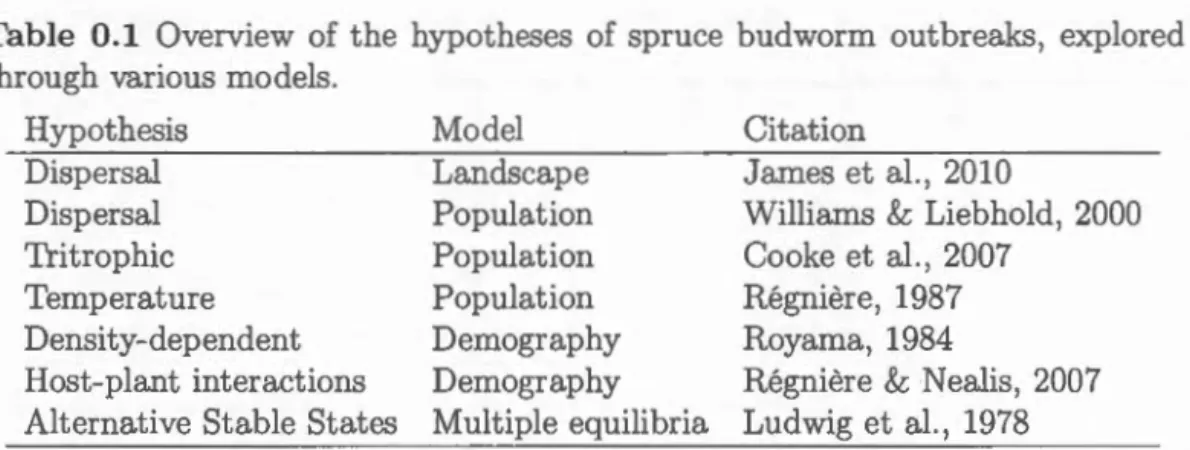
0.1 Overview of the hypotheses of spruce budworm outbreaks, explored through various models. . . . . . . . . . . . . . 15 1.1 Conclusions from comparing the results from bath spatially-implicit

and -explicit FIRF models under different types of density-dependence. 'Yes' indicates that outbreaks occur under at least sorne parame-ter values. For the local stability analysis of the spatially-implicit madel, outbreaks (damped or sustained oscillations) are indicated by the presence of complex eigenvalues. Outbreak cyclicity is as-sessed by numerical simulations. . . . . . . . . . . . . . . . . . 44 2.1 The potential climate variables used in the analysis and their time

lags tested. The interpolated values covered each cell in the study area (Fig. 2.1 b) from 1965- 2013. From McKenney et al., 2011. Bottom five lines, the types of climate randomizations. . . . . . . 55 2.2 Madel selection results on defoliation FI transitions. The three

best climate variables were summer maximum temperature

t -

3, summer minimum temperature t

-

3 and number of growing degree days

t -

2. The variables had third-degree response terms. K

=

the number of variables. . . . . . . . . . . . . . . 64 3.1 Madel states and default parameters used in simulations.

A.1 Parameters of full madel.

B.1 AIC results, backward selection. Madel selection results on MI transitions, with 1,2 and 3-degree response terms and estimated on all data. Each AIC is obtained when carrying out a glm with

87

116

all climate variables except that one. The variable when removed results in the highest AIC is the most important variable. . . . . . 129

B.2 AIC results, backward selection. Model selection results on IM transitions, with 1,2 and 3-degree response terms and estimated on all data. Each AIC is obtained when carrying out a glm with all climate variables except that one. The variable when removed results in the highest AIC is the most important variable. . . . . . 130 B.3 Model selection results on defoliation FI transitions also testing

submodels of the effect of forest type and years since outbreaks. We removed all data points where the number of years since the last outbreak and the forest type was unknown, which resulted in a smaller data set (192 056 instead of 235 744 observations). The three best climate variables were summer maximum temperature

t-

3, summer minimum temperature t- 3 and number of growing degree days

t-

2. The variables had third-degree response terms. K

= the

number of variables. . . . . . . . . . . . . . . . . . . . . 131 B.4 The total transition events, when tO is either Infected or Forest

with no outbreaks (K

<

0.01) and with outbreaks (K > 0.01). . . 132 B.5 The total transition probabilities, when tO is either Infected, Forest

with no outbreaks (K < 0.01) and with outbreaks (K > 0.01). . . 132 B.6 Model selection results on dieback IF transitions. The predictors

had third-degree response terms. K

=

the number of variables. The random residuals are estimated on half of the data selected randomly, and repeated 10 times. . . . . . . . . 132

Figure

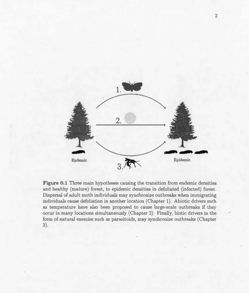
0.1 Three main hypotheses causing the transition from endemie densi-ties and healthy (mature) forest, to epidemie densities in defoliated (infected) forest. Dispersal of adult moth individuals may synchro-nize outbreaks when immigrating individuals cause defoliation in another location (Chapter 1). Abiotic drivers such as temperature have also been proposed to cause large-scale outbreaks if they oc-cur in many locations simultaneously (Chapter 2). Finally, biotic drivers in the form of natural enemies such as parasitoids, may

Page

synchronize outbreaks (Chapter 3). . . 2

0.2 The spruce budworm lifecycle.

0.3 Top, Dendrochronological data from Boulanger et al. (2012) indi-cating the percentage of beamsjtrees showing growth reduction due to spruce budworm defoliation in one location in southern Quebec. Bottom, wavelet analysis of dendrochronological data, indicating the periodicity in each year. Defoliation has a significant peri-odicity of 35 years during 1850-2000 (significant periodicities are surrounded by black lines). 1650-1850 no dominant period was

4

detected at this location. . . . . . . . . . . 7 0.4 Episodic occurrences of defoliation and dieback events. Left, the

total proportion of infected locations in spruce budworm defoli-ation data. Middle, the number of defolidefoli-ation transitions (from non-defoliated to defoliated forest). Right, the number of dieback transitions (from defoliated to non-defoliated forest). The total number of locations was 6 446, and see section 2 for more details on data. . . . . . . . . . . . . . . . . . . . . 9 0.5 Top row, densities of host species (red line, note log scale) and

percentage parasitized for (black line) three defoliator species over time. Bottom row, phase plots with host density plotted against percentage parasitized of the same species. Data from Myers

&

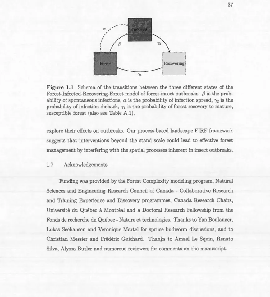
Cory (2013). . . . . . . . . . . . . . . . . . . . . . . 11

1.1 Schema of the transitions between the three different states of the Forest-Infected-Recovering-Forest madel of forest insect outbreaks. {3 is the probability of spontaneous infections, a is the probability of infection spread, "'(2 is the probability of infection dieback, "'(1 is 'the probability off01·est recovery to mature, susceptible forest (also see Table A.1). . . . . . . . . . . . . . . . . . . . . 37 1.2 The presence of cyclic out breaks of the density-dependent

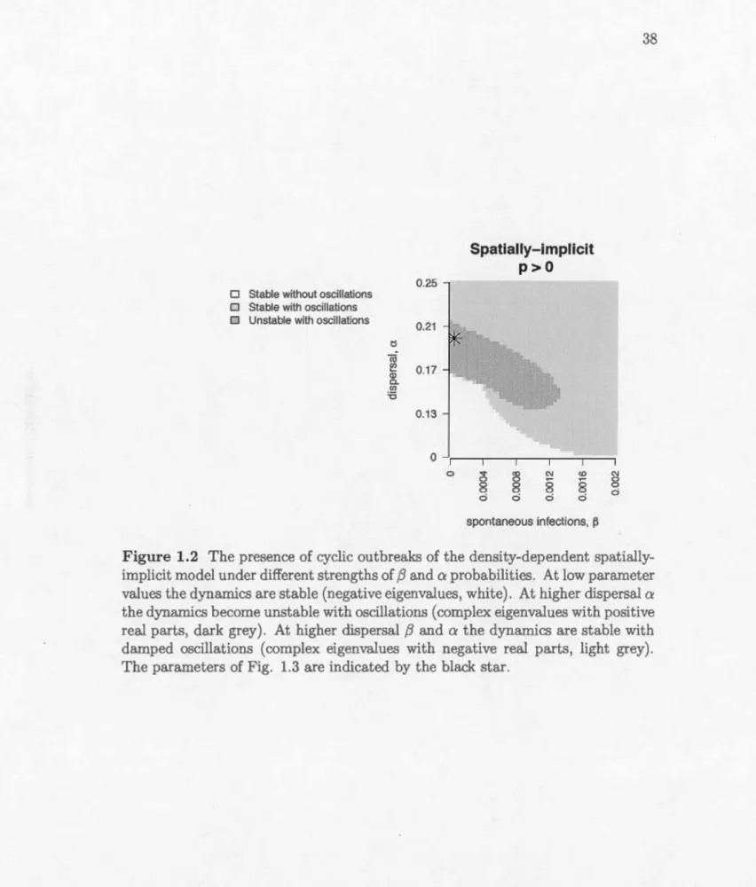
spatially-implicit madel under different strengths of {3 and a probabilities. At law parameter values the dynamics are stable (negative eigenval-ues, white). At higher dispersal a the dynamics become unstable with oscillations ( complex eigenvalues with positive real parts, dark grey). At higher dispersal {3 and a the dynamics are stable with damped oscillations ( complex eigenvalues with negative real parts, light grey). The parameters of Fig. 1.3 are indicated by the black star. . . . . . . . . . . . . . . . . . . . . . . . . . 38 1.3 Examples of FIRF madel simulations with the proportion of each

forest state over time. A, Spatially-implicit madel with density-independent dispersal

(p

=

0) and B density-dependent dispersal

(p

> 0). C

, spatially-explicit îmmigration-driven density-dependent dispersal

(p

> 0).

D, spatially-explicit emigration-driven dispersal madel

(p

>

0). The parameters used are a

=

0.2, {3

=

0.001, "YI = 1/40, "'(2 = 1/3 and p = 0.4. We show the dynamics with {3

= 0 in Figure A.3.

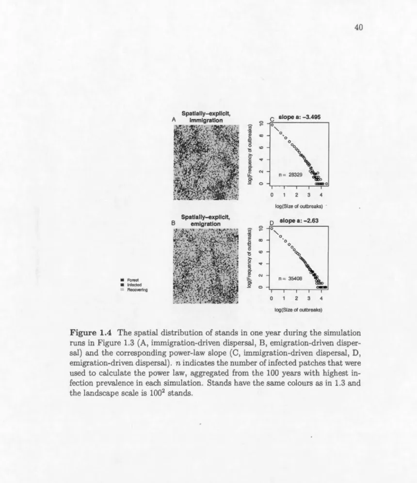
. . . . . . . . . . . . . . . . . . . . . . 39 1.4 The spatial distribution of stands in one year during the simulation

runs in Figure 1.3 (A, immigration-driven dispersal, B, emigration-driven dispersal) and the corresponding power-law slope (C, immigration-driven dispersal, D, emigration-driven dispersal). n indicates the number of infected patches that were used to calculate the power law, aggregated from the 100 years with highest infection preva-lence in each simulation. Stands have the same colours as in 1.3 and the landscape scale is 1002 _{stands. . . . . . . . . . . . . 40}

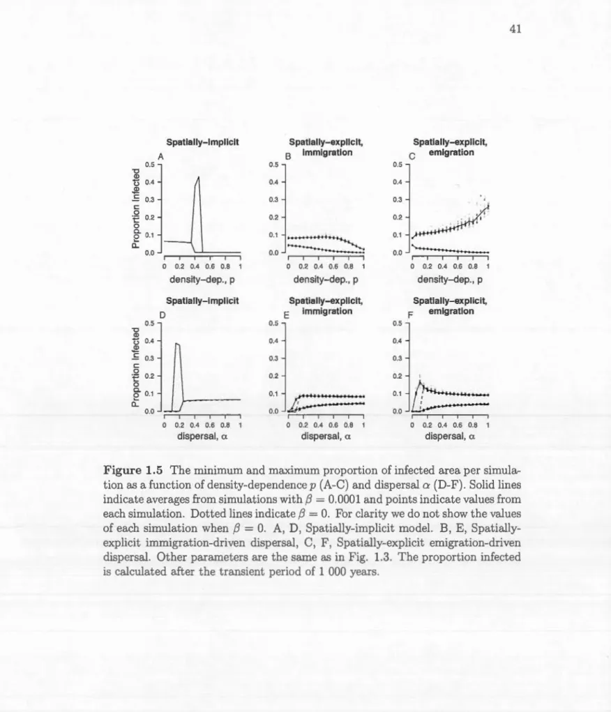
1.5 The minimum and maximum proportion of infected area per sim-ulation as a function of density-dependence p (A-C) and disper-sal a (D-F). Solid lines indicate averages from simulations with

f3

=

0.0001 and points indicate values from each simulation. Dot-ted lines indicate

f3

=

O. For clarity we do not show the values of each simulation when

f3

=

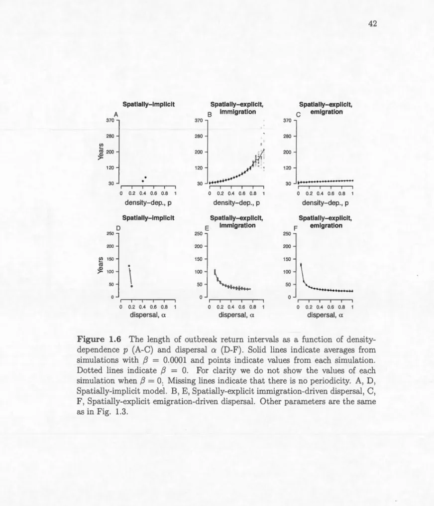
O. A, D, Spatially-implicit madel. B, E, Spatially-explicit immigration-driven dispersal, C, F, Spatially-explicit emigration-driven dispersal. Other parameters are the same as in Fig. 1.3. The proportion infected is calculated after the tran-sient period of 1 000 years. . . . . . . . . . . . . . . . . . . . 41 1.6 The length of outbreak return intervals as a function of

density-dependence p (A-C) and dispersal a

(D-F).

Solid lines indicate averages from simulations with f3

=

0.0001 and points indicate val-ues from each simulation. Dotted lines indicate f3 = O. For clarity we do not show the values of each simulation when f3

= O. Missing

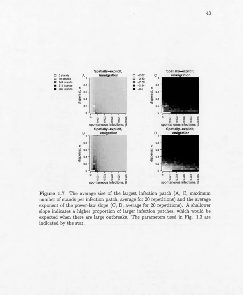
lines indicate that there is no periodicity. A, D, Spatially-implicit madel. B, E, Spatially-explicit immigration-driven dispersal, C, F, Spatially-explicit emigration-driven dispersal. Other parameters are the same as in Fig. 1.3. . . . . . . . . . . . . . . . . . . . 42 1.7 The average size of the largest infection patch (A, C, maximum

number of stands per infection patch, average for 20 repetitions) and the average exponent of the power-law slope (C, D, average for 20 repetitions). A shallower slope indicates a higher proportion of larger infection patches, which would be expected when there are large outbreaks. The parameters used in Fig. 1.3 are indicated by the star. . . . . . . . . . . . . . . . . . . . . . . . . . . . . . . . 43 2.1 Left, the proportion of outbreaks over time, expressed as the

pro-portion of cells in the infected state. Right,. the geographie extent of the study area in Quebec province, Eastern Canada. Each square is a 'cell' (6 446 in total) and the colour indicates its state: Dark grey (red online) is defoliated/infected, grey (green online) is for-est non-infected cell in 2015. Grey areas were never infected and excluded from the analysis. . . . . . . . . . . . . . . . . . . . 51 2.2 Schematic representation of a metapopulation approach to forest

insect outbreaks, indicating the forest F and infected 1 states. The arrows indicate the parameters that set the state transitions infec-tion F--+ 1 and dieback 1--+ F. . . . . . . . . . . . . . . . 54

2.3 .Map of aK calculated from the cells defoliated in 2013 (in clark grey, red online). The dispersal kernel K was calculated using the

negative exponential kernel with 8

= 10. . . . .

. . . . . . . . . . 61

2.4 The simulated proportion of infected cells with different types of

spatiotemporally autocorrelated climate. Dotted lines indicates the

observed outbreaks, and each thin line indicates one simulated

out-break. . . . . . . . . . . . . . . . . . . . . . . . . . . . . . . . . . 65

2.5 Summary results from simulation model. Horizontal dotted lines

indicate the values in the observed outbreaks. Each plot shows

the values from 100 simulations. Boxes encompass the 25%- 75%

quartiles of the data, with the median indicated by the thick line

through the centre of each box. Whiskers extending from the box encompass the 95% quartiles, and extreme observations are shown as circles. a, Maximum proportion of infected area. b, Standard de-viation in the simulated proportion of infected area I. c, Temporal

autocorrelation with a 1 year time lag. d, Range of positive

tempo-ral autocorrelation (in years). e, Maximum number of contiguous outbreak clusters per simulation. f, Largest contiguous outbreak

elus ter size per simulation ( number of cells). . . . . . . . . 66

3.1 Effect of each trophic level on underlying trophic levels. Vertical

line thickne s indicates interaction strength. Horizontal arrows

in-dicate time. Species sizes is proportional to the density of each

trop hic level (not body size). The forest appears defoliated only in the host-controlled state, and both parasitoid-and hyperparasito id-controlled forest is healthy, non-defoliated. Note that hyp erpara-sitoids have a strong effect on both parasitoid and host, in contrast to trophic relationships where a stronger effect on one trophic level

leads to a weaker effect on the next trophic level (alternating not

additive). . . . . . . . . . . . . . . . . . . 78

3.2 Metacommunity model with the three trophic levels with

host-controlled, parasitoid-controlled and hyperparasitoid-controlled states, showing states and transitions. Dotted lines indicate second-order rates that depend on the concentration of both states. See Table 3.1 for description of state and parameters. . . . . . . . . . . . . 79

3.3 Example simulations with only parasitoids (left column, A, D, G), both parasitoids and hyperparasitoids (middle column, B, E, H), and only hyperparasitoids (right column, C, F, I), in both spatially-implicit (top row) and -explicit models (middle row). The bottom row shows an example landscape from the spatially-explicit simu-lations. If a (hyper- )parasitoid was present, its exclusion rate ep

xii

(ehp) was 0.001. AU other parameters are as in Table 3.1. 92 3.4 Effect of hyperparasitoid control chp and exclusion ehp rates on

outbreak size, i.e. proportion landsca,pe in state I. Each value indicates the average maximum infected proportion from all simu-lations with that parameter combination. Simulations were carried out with other parameters as in Table 3.1. .. . . .. . . .. . . . · 93 3.5 Effect of host dispersal rates into parasitoid-controlled and

hyperparasitoid-controlled forest on outbreak size, i.e. proportion landscape in state I. The diagonal white line indicates asbwv

=

asbw~tv· Simulations were carried out with all other parameters as in Table 3.1. . . . . 94 A.1 Illustration of the density-dependent dispersal function. The lines

show the nonlinear dispersal function

f (

I)

=

JP I un der different values of p and a

=

1. . . . . . . . . . . . . . . . . . . . . . . . . 116 A.2 Neighborhood considered for the calculation of the density-dependent

dispersal function f(I) for immigration and emigration mo dels (de-lineated by black lines). For immigration (a-c), the neighborhood consists of the 8 stands surrounding the arrival stand F. lp counts the relative number of infected stands in the neighborhood. For em-igration ( d-f), the neighborhood consists of the 8 stands surround-ing the origin stand I.

J1

counts the relative number of infected stands in the neighborhood. . . . . . . . . . . . . . . . . 117 A.3 Examples of FIRF model simulations without spontaneous

out-breaks

(fJ

= 0). The same figure

as Figure 2 in the manuscript. a, Spatially-implicit model with density-independent dispersal (p

=

0). b, Spatially-implicit mo del with density-dependent dispersal

(p

>

0). c, spatially-explicit immigration mo del with density-dependent dispersal (p

> 0)

. d, spatially-explicit emigration model with density-dependent dispersal (p

> 0)

. e and f show the spatial distribution of stands from the simulation runs in c and d. The parameters used are a

=

0.2,

fJ

=

0, rl

=

1/40, 12

=

1/3 and p

= 0.4. .

. . . . . . . . . . . . . . . . . 118

A.4 Examples of spatially-explicit FIRF model simulations with low and high emigration-driven dispersal (a). a, spatial distribution of stands with low dispersal a

=

0.2 and b high dispersal a

=

0.5. The corresponding power-law slopes (solid line) from high c and low dispersal d. The parameters used are (3 = 0.0001, 'Yl = 1/40, ")'2

= 1/3 and p

= 0.4.

. . . . . . . . . . . . . . . . . . . 119 A.5 Examples of spatially-explicit FIRF model simulations with low

and high immigration-driven dispersal (a). a, spatial distribution of stands with low dispersal a = 0.2 and b high dispersal a = 0.5. The corresponding power-law slopes (solid line) from high c and low dispersal d. . . . . . . . . . . . . . . . . . . . . . . . . . 120 B.1 Proportion of variance explained by the first 25 axes of a PCA on

the dispersal variables K . . . . . . . . . . . . . . . . . . 123 B.2 Proportion of variance explained by the first 25 axes of a PCA on

the climate variables . . . . . . . . . . . . . . . . . . . . . 124 B.3 Examples of K with different values for 8, the effect of distance to

defoliated cells. . . . . . . . . . . . . . . . . . . . . . . . . 125 B.4 The likelihood profile from selection of the best dispersal kernel

Ki with first, second and third degree response functions. The esti-mated AIC with dispersal kernels calculated with different 8 values, from a forwards stepwise logistic regression. The autologistic and negative exponential kernels are both tested with infection distri-butions from one and two years previously. . . . . . . . . 126 B.5 Selection of best climate variable. AIC results of backward model

selection results on FI infection transitions, third-degree response terms. . ..

B.6 AIC results, backward selection. Model selection results on IM transitions, response terms with 3 degrees and estimated on all

127

B.7

B.8

!

l_

The predicted climate predictions E estimated with a logistic re-gression with third-degree relationships. Top left, EFI, mean prob-ability of forest infection, calculated from all years. White colours indicate a high probability of a forest cell transitioning from the forest state F to infected I, and black colours indicates a low prob-ability of transition (the forest stays as forest). These probabilities are only based on climate and do not include the effect of di sper-sal. Top right, EIF, mean probability of dieback, calculated from all years. White colours indicate a high probability of a forest cell transitioning from the infected state I to the forest state F, and black colours indicates a low probability of transition (the infected area stays infected). Bottom left, The effect of one climate vari-able (selected by backward AIC) on the probability ofF I infection. The black line shows the probability of spontaneous infection (Ki

= 0.0)

and the grey line shows the probability of infection when the dispersal kernel Ki

>

0.1. The grey bars show the observed trans i-tions. Bottom right, The effect of one climate variable (selected by backwards AIC) on the probability of IF dieback. The grey bars show the observed transitions. . . . . . . . . . . . . . . . . . . . . The predicted climate predictions E and dispersal parameters. Bot-tom, the mean predicted probabilities of infection EFI (red lines) and dieback E1F (green lines), in all cells. The solid red line is the annual observed total proportion of infected forest. Top, cross-correlation wavelet between EFI and EJF. The colours represent the power of the period of the fluctuations, from clark blue (low val-ues), to clark red (high values). The arrows show the phase angles between the fluctuations in the climatic predictions. Arrows pa int-ing left indicate asynchrony in values and arrows painting clown indicate that the EFI fluctuates before the EIF by a quarter period

(90

°)

.

133

Déterminer les causes de la répartition et des fluctuations des espèces est un important défi en écologie. Un exemple spectaculaire de fluctuations d'espèces est les épidémies d'insectes ravageurs, caractérisées par des densités élevées de population à travers un paysage. Malgré de nombreuses études empiriques et théoriques des fluctuations des espèces, les causes des épidémies sont loin d'être bien comprises et une meilleure compréhension de celles-ci pourrait en améliorer la gestion. Cette thèse porte sur les trois principales hypothèses proposées pour expliquer la synchronie des épidémies à large échelle spatiale-le climat, la di sper-sion, et les ennemis naturels. J'ai couplé des modèles statistiques et mécanistiques pour tester les trois hypothèses dans le contexte d'un insecte ravageur bien étudié ; la tordeuse des bourgeons de l'épinette ( Choristoneura fumiferana). Le mod-èle a été paramétré avec des cartes spatiotemporelles de défoliation comme un proxy pour les densités de population. Les simulations indiquent que la di sper-sion non linéaire, comme prévu par l'effet Allee, était important pour produire des épidémies cycliques et synchrones. L'analyse statistique des cartes spatio tem-porelles d'épidémie a montré que la dispersion se produit plus souvent entre les cellules voisines, mais que la dispersion à longue distance a également lieu occa-sionnellement. Des mécanismes abiotiques tels que le climat peuvent également synchroniser les épidémies à grande échelle (effet Mor an). Des modèles statistiques ont montré que la dispersion avec toutes les variables climatiques reproduisent bien les épidémies de tordeuse observées. Ces estimations ont été utilisées en tant que paramètres dans des simulations pluriannuelles. L'autocorrélation t em-por·elle, sous forme de plusieurs années avec un climat favorable a augmenté l'effet Moran et encouragée les épidémies. Cependant, même avec l'autocorrélation spa-tiotemporelle observée et la dispersion, le modèle a été incapable de reproduire la distribution spatiales en grappe des épidémies. Enfin, les meécanismes biotiques, sous la forme de divers ennemis naturels, peuvent affecter la dynamique des in-sectes, et les parasitoïdes en particulier peuvent les déstabiliser. Pour étudier le rôle des parasitoïdes, j ai construit un modèle de métacommunauté dans lequel la dynamique de la tordeuse est déterminée par des interactions avec les parasitoïdes. Le modèle indique que hyperparasitoïdes de niveau supérieur peuvent interrompre le contrôle parasitoïde et générer des épidémies. Dans cette thès , j réinterprète les épidémies d'insectes ravageurs comme un processus de métapopulation, et comme les modèles de métapopulation sont analogues à des modèles épidémi-ologiques, mon modèle peut être utile pour élaborer des stratégies de gestion. Le

XVI

comportement de dispersion de la tordeuse estimé peut être utilisé pour planifier la récolte des arbres tout en minimisant la dispersion et donc les épidémies. La surveillance des hyperparasitoïdes pourrait indiquer si une épidémie se produira

bientôt. En conclusion, j'ai démontré que l'autocorrélation climatique temporelle

pourrait amplifier les fluctuations des populations d'insectes dans le temps, et que

la dispersion et les ennemis naturels interagissent pour regrouper spatialement les épidémies.

Mots-clé: métacommunauté, métapopulation, épidémies d'insectes ravageurs,

Determining the causes of species distributions and fluctuations is an

impor-tant ecological challenge. One striking type of ecological dynamics are outbreaks

of insect pests, defined as high population densities synchronously throughout a landscape. Despite many empirical and theoretical studies of species fluctuations, what drives outbreaks is far from well understood but could improve management.

This thesis focused on the three main hypotheses proposed to synchronize

out-breaks - climate, dispersal, and natural enemies. I coupled statistical and

mecha-nistic models to test all three hypotheses for a well-studied insect pest, the spruce

budworm ( Choristoneura fumiferana). The resulting metapopulation mo del was

parameterized with spatiotemporal defoliation maps as a proxy for population

densities. Simulations indicated that nonlinear dispersal, as expected from the

Allee effect, was important to produce synchronous, cyclic outbreaks. Statistical

analysis of spatiotemporal outbreak maps showed that dispersal occurred most often between neighbouring stands, but that occasional long-distance dispersal also took place. Abiotic drivers such as climate may also synchronize large-scale outbreaks (M01·an effect). Spatiotemporal climate and dispersal variables were tested to disentangle their relative importance. Statistical models showed that dispersal with all climate variables best fit observed budworm outbreaks. These estimates were employed as parameters in multi-year simulations to identify if climate autocorrelation synchronizes outbreaks. Temporal autocorrelation in the

form of consecutive suitable years 'enhanced' the spatial Moran effect and

en-couraged outbreaks. However, even with observed spatiotemporal autocorrelation

and dispersal, the model did not reproduce the spatial clusters of observed

out-breaks. Finally, biotic drivers in the form of various natural enemies may affect

outbreaks, and parasitoids in particular destabilize dynamics. To investigate the role of parasitoids I constructed a metacommunity model in which budworm

dy-namics were driven by parasitoid interactions. The model indicated that high

er-level hyperparasitoid can interrupt parasitoid control and generate. out breaks. In

this thesis, I reinterpreted insect pest outbreaks as a metapopulation process, and

since metapopulation models are analogous to epidemiological models, my model can employ spatial epidemiological strategies to elaborate management strategies. The estimated budworm dispersal behaviour can be used to plan harvesting that minimizes dispersal and thus outbreaks. Monitoring hyperparasitoids could indi-cate if an outbreak will occur soon. In conclusion, I demonstrated that temporal

climate autocorrelation may amplify insect population fluctuations in time, and that dispersal and natural enemies interact to spatially cluster distributions.

0.1 Overview

Determining the causes of species distributions and fluctuations is an im-portant ecological challenge. What regulates whether a species is present at a particular time and place? One striking example of ecological dynamics are out-breaks, defined as synchronously high population densities throughout a landscape (Liebhold et al., 2004). Out breaks are so striking be cause the tin y insects reach

such high densities that they cause enormous impacts on their resource (Cooke

et al., 2007). Large-scale spatiotemporal population fluctuations are also of inter -est because understanding why certain species fluctuate can help us to understand why other species have stable distributions. Ultimately, knowledge of ecological mechanisms can be employed to improve ecological management, whose goal is either to stabilize (prevent extinction) or desynchronize (prevent outbreaks) eco-logical dynamics. Here I developed a simple yet inclusive framework to model species outbreaks that focuses on the presence or absence of insect disturbance in the form of forest defoliation. The model is analogous to a metapopulation model (Levins, 1969), which was created to improve pest management but has rarely been applied to this goal. To make the metapopulation model more relevant, I extended it to represent and investigate the factors that drive outbreaks.

This thesis tested the three main hypotheses that are proposed to explain synchronous out breaks - dispersal, elima te, and nat ur al enemies (Figure 0.1). The intrinsic hypothesis of outbreaks, dispersal, may synchronize outbreaks when individuals from a single population disperse throughout the landscape (Chapter

1.

-2.

Endemie

3.~

Epidemie

Figure 0.1 Three main hypotheses causing the transition from endemie densities and healthy (mature) forest, to epidemie densities in defoliated (infected) forest. Dispersal of adult math individuals may synchronize outbreaks when immigratiùg individ uals cause defoliation in another location ( Chapter 1). Abiotic drivers su ch as temperature have also been proposed to cause large-scale outbreaks if they occur in many locations simultaneously (Chapter 2). Finally, biotic drivers in the form of natural enemies such as parasitoids, may synchronize outbreaks (Chapter 3).

1). Abiotic drivers such as spatially autocorrelated environmental variation has

also been proposed to synchronize the dynamics of independent populations (the

Moran effect, Chapter 2). Finally, biotic drivers in the form of natural enemies may affect outbreaks (Chapter 3).

I explored these synchronizing mechanisms in what is possibly the most

throughly studied insect species: the spruce budworm (section 0.2). Quebec is in the middle of a large-scale outbreak in 2016; it is remarkable that yet again the out-breaks have returned every rv30 years. The budworm is an ideal study organism for such an in-depth investigation, because it displays rich dynamics in time and space. Theoretical, mathematical models are necessary to improve understand-ing of outbreaks, because merely description does not improve understanding of

mechanisms driving them, and landscape-scale experiments are unfeasible. The

objective of this thesis was to develop a framework flexible enough to test all three outbreak-causing mechanisms but realistic enough to refl.ect biological knowledge (section 0.4). To develop this framework I integrated other modelling app.roaches,

namely metapopulation, multiple equilibria and epidemiological models. The

re-sulting model was suitable to evaluate the intrinsic (Chapter 1), abiotic (Chapter 2) and biotic (Chapter 3) synchronizing mechanisms of landscape-wide, multi-year

budworm outbreaks.

0.2 Spruce budworm as an example system

The Eastern spruce budworm ( Chorisoneura fumiferana Lepidoptera:

Tor-tricidae) is considered the most serious pest in the boreal and sub-boreal forests of North America (NRC, 2013). Given that budworm outbreaks cause large-scale defoliation and mortality of economically important trees, factors affecting its reproduction and survival are well-understood. The budworm completes its life cycle in a ingle year (Figure 0.2). The larvae emerge from diapause in spring

4th, 5th, 6th INSTAR

, ...

~

3rd

iNSTAR

lst INSTAR

WINTER HIBERNATION 2nd INSTAR

Figure 0.2 The spruce budworm lifecycle.

and feed on current-year buds (NRC, 2013). Precipitation during sprin.gtime

lar-val emergence may lower survival rates (Lucuik, 1984). The larvae establish in a

feeding site and develop through four instars, and summer temperatures strongly

affect development rates and survival (Régnière, 1987). Summer temperatures

modify fecundity and survival rates which influences tree defoliation levels (Blais,

1958; Gray, 2008). Pupation takes place in june, and adult maths emerge 10 days

later. Adults find each other to mate with the help of pheromones, and the female

lays around 200 eggs (Régnière et al., 2012). If densities are too low, mate-finding is more difficult, so the Allee effect has been observed in the budworm (Régnière

et al., 2012). When eggs hatch the first instar larvae emerges and then spins a

co-caon to hibernate in un til the following spring (Nealis & Régnière, 2009). Extreme

low and high winter temperatures may cause overwintering mortality (Régnière

et al., 2012).

Budworm densities vary over orders of magnitude between endemie and

epidemie periods, leading to tree defoliation (Royama, 1992; Sanders, 1996; Cap

densities per kilo of foliage feU from 2 233 to 11 during eight years. Higher defo-liation rates in a stand influence budworm fecundity and survival rates (Régnière & Nealis, 2007). Especially young larvae experience higher mortality in heavily defoliated stands (Nealis & Régnière, 2004b; Fuentealba & Bauce, 2012). Defoli-ation destroys buds, causes abnormal growth of new twigs, and a reddish colour of dried needles. The budworm is a selective feeder, preferring mature balsam fir (Abies balsamea) and white spruce (Picea glauca) stands over other forest types (Royama et al., 2005; Nealis & Régnière, 2004b; Hennigar et al., 2008). High rates of defoliation decrease the photosynthetic capacity of the host tree (Baskerville & Kleinschmidt, 1980). One year of epidemie budworm densities weakens the tree,

and if defoliation continues over several years tree mortality occurs (NRC, 2013). Bergeron et al. (1995) showed that average tree mortality within a stand was 50%, and occasionally reached 100%. Tree mortality increases with stand age but much variability remains unexplained, so it is likely that regional factors beyond stand age also determine tree mortality (Bergeron et al., 1995).

Budworm individuals can disperse large distances but it is unknown how much immigration is necessary to initiate defoliation elsewhere. Adult budworm moths can efficiently travel 48 km (Anderson & Sturtevant, 2011), and the maxi-mum recorded distance is 450 km (Greenbank, 1956, 1980). Suitable meteorolog-ical and atmospheric conditions favour successful long distance dispersal (Stur te-vant et al., 2013). The moths emigrate in larger numbers from defoliated stands with high budworm densities (Royama, 1984; Régnière & Nealis, 2007). Fecun-dities of adults is represented by the local egg to moth ratio (E/M ratio). A high E/M ratio compared to the apparent fecundity of moths can indicate that dispersal has occurred to a site (Royama, 1984; Nealis & Régnière, 2004b). Ge

-netic studies show that gene flow between populations is high, indicating strong di persal ability (James et al., 2015).

The budworm has many natural enemies, including predators, parasites and parasitoids (Régnière, 2001; Huber et al., 1996; Eveleigh et al., 2007). During budworm outbreaks, certain warbler species increase in population densities (Ve -nier et al., 2009; Venier & Holmes, 2010). High-density budworm populations may experience parasitic mite infections (Houseweart, 1980). By far the best-studied natural enemy group are the parasitoids, with more than one hundred parasitoids and hyperparasitoids (Eveleigh et al., 2007; Smith et al., 2011). Parasitoids are often wasps with specifie adaptations to attack their hosts (i.e. the budworm, Godfray & Shimada, 1999). During endemie periods the observed mortality rates from parasitoids are high (50-90% in Seehausen et al., 2014,40-70% in Cappuccino et al., 1998, and all primary parasitoids, 62-75% in Dowden et al., 1950). Less is known of parasitoid mortality rates during epidemie periods, but the identity of the species present may change due to parasitoid life history. Parasitoids can e i-ther be univoltine and have one generation and one host per year, or bivoltine and have two generations and need two hosts to complete a life cycle; the budworm and an alternate host. Bivoltine parasitoids are limited by the density of the alter -nate host and can only partially increase in density to respond to high budworm densities (Régnière, 2001). The identity of alternate hosts is mostly unclear, but they may be present in deciduous forests (Cappuccino et al., 1998). Through their impact on natural enemies, surrounding forest composition can increase parasitoid densities, and ultimately also affect budworm densities (Cappuccino et al., 1998; Su et al., 1996).

Budworm outbreaks can be characterized through spatial, temporal and spatiotemporal data in increasing detail. Data on population-leve! density and survival time series are time-and labour-intensive to collect, so are only available for a few locations (e.g. Royama et al., 2005; Régnière & Nealis, 2007; Pureswaran et al., 2016). Chronicling older out breaks is possible using dendrochronology

Proportion trees aHected par year 0.5 1500 1600 1700 1800 1900 2000 '<t "0 <0 0 -~ ~ a_ 00 N 1600 1700 1800 1900 2000 Ti me

Figure 0.3 Top, Dendrochronological data from Boulanger et al. (2012) indicating the percentage of beams/trees showing growth reduction due to spruce budworm defoliation in one location in southern Quebec. Bottom, wavelet analysis of den-drochronological data, indicating the periodicity in each year. Defoliation has a significant periodicity of 35 years during 1850-2000 (significant periodicities are surrounded by black lines). 1650-1850 no dominant period was detected at this location.

because budworm defoliation reduces tree ring growth (Figure 0.3, Boulanger et al., 2012). The most comprehensive, multi-year and landscape-scale data is

m the form of defoliation maps. Aerial defoliation surveys have been carried out 1968 - 2015 in Quebec and track the location of defoliated forest each year (Figure 2.1, section 2 for more details on data). Defoliation has been used as a proxy for population densities because insect densities have a large effect on forest ecosystems via tree defoliation and mortality ( e.g. Williams & Liebhold,

2000; Bj0rnstad et al., 2002).

Over time, the prevalence of budworm outbreaks are positively autocorr e-lated, and more specifically they appear to alternate between chaotic and cyclic

dynamics. Outbreak dynamics may change over time; they may be non-stationary.

A temporally explicit analysis indicates that outbreaks have occurred approx

i-mately every 35 years over the last 150 years and more irregularly earlier (Figure

0.3, wavelet analysis, Cazelles et al., 2008, see also Simard et al., 2006). Chao tic

dynamics may be generated from nonlinear interactions between species life stages

or between multiple species (Hastings et al., 1993; Benincà et al., 2008; Costantino et al., 1997). The complete dendrochronological time series is chaotic (maximal

Lyapunov exponent À

=

0.332, data from 0.3, analyzed using Narzo & Narzo, 2010). However, the dynamics are not chaotic when analyzing only the last 150

years

(.>.

=

- 0.097), during which the dynamics may be cyclic or rand0m. De n-drochronology may generate time series with errors in older data and only repr e-sents dynamics in one one severallocation, therefore the results are not conclusive. Describing budworm dynamics with combined spatiotemporal statistics is complicated because raw defoliation data is binary (presence or absence of defo

li-ated trees) and many methods of analysis require continouos data (e.g. travelling waves, Bj0rnstad et al., 1999). To describe spatiotemporal variation in local de -foliation, one can assess what proportion of locations transition from defoliation

.

.

.

'\

;

j.J..L

~

.

:].!

\

§

j

~~

1 /·

1 1 •

.

_~

• • 1

0

.·

-~ .,..,.-...·

-

1 ••• • . .

...

1970 2014 1970 2014 1970 2014

Figure 0.4 Episodic occurrences of defoliation and dieback events. Left, the total

proportion of infected locations in spruce budworm defoliation data. Middle, the

number of defoliation transitions (from non-defoliated to defoliated forest). Right, the numbE?r of dieback transitions (from defoliated to non-defoliated forest). The

total number of locations was 6 446, and see section 2 for more details on data.

to non-defoliated, and vice versa, in each year. These transitions are episodic, i.e. multiple transitions interspersed among periods of range stasis, and they occur with greater variability than the resulting total defoliation (Figure 0.4, Johnson

et al., 2006).

For several reasons, biological knowledge and statistical descriptions of the spruce budworm cannot explain why large-scale outbreaks occur. First, how local factors such as climate and natural enemies together translate to local population densities and stand defoliation is already complex and subject to many studies (Royama, 1992). Second, local defoliation may cycle due to local mechanisms,

but other, regional mechanisms may cause this defoliation to take place simul

ta-neously throughout the landscape (Peters et al., 2004a). Third, local and regional mechanisms may influence each other (Raffa et al., 2008). There is a gap between

local knowledge and the large-scale mechanisms that may synchronize outbreaks.

In other words, it is not the local destructiveness but the extent of the synchrony

that should be studied to understand outbreaks (Cooke et al., 2007). 1 will now

discuss the three main mechanisms that are thought to synchronize outbreaks on a landscape-scale.

0.3 Three mechanisms that synchronize outbreaks

Dispersal synchronizes local populations because individuals from a high-density population spread and increase population densities elsewhere. This is an intrinsic mechanism because it only depends on the species itself. Williams &

Liebhold (2000) found that long-distance dispersal together with climatic spatial autocorrelation were the strongest determinants of budworm outbreaks. How-ever, to build their simulation model they chose parameter values that produced outbreaks, so the parameter values may not be biologically realistic for the bud-worm. Dispersal must be strong to synchronize insect population cycles, however dispersal strength is difficult to estimate (Royama et al., 2005; Myers & Cory, 2013).

The Moran effect states that if two populations have similar population dynamics, the degree of correlation between them should be the same as the correlation in weather variables influencing their respective dynamics (Moran, 1953). The cross-correlation between two populations densities, rp, should be identical to the cross-correlation between two environmental variables, r (Massie et al., 2015). Experiments can control the environmental drivers and quantify the strength of the Moran effect (Massie et al., 2015; Vasseur & Fox, 2009). Under natural conditions, the Moran effect has been identified in isolation from other mechanisms (without dispersal or natural enemies, Grenfell et al., 1998; Stenseth et al., 1999; Post

&

Forchhammer, 2002). In the field it is difficult to disentangle the effect of climate from other processes affecting population dynamics.

Synchronous fluctuations of interacting natural enemies may synchronize fluctuations of the fluctuating species (Bj0rnstad et al., 2002; Cattadori et al., 2005; Allstadt et al., 2013). For example, predatory birds synchronize vole pop-ulations in multiple locations (Ims & Andreassen, 2000). In spatial theoretical

Western Tent Caterplllar Larch Budmoth Autumnal Moth

~ '

~

oooo

1000

l~

r

[ : 100

~

-~

u 100 _{L4o ~}

~ 10 ~ 20 ~

. c , •~o ₀!>.

i?:'

~

~

!

'oo

'li$

·~ 1&+02

j

n :~ ~

"0 1&+00 • 40 ...

~ 1 20 ~

..c le-02 - 0 ;sf?.

0 5 10 15 20 25 0 10 20 30 40 0 5 10 15 20 25 30

lime lime lime

~

VJ

':

60

l

-

~

~ 40 -·

a. 20 ..

'$~ 0

·-1 10 100 1000 1e-01 le..-01 1e+03 le-02 1e+00 19+02

host densitv host density host densitv

Figure 0.5 Top row, densities of host species (red line, note log scale) and per-centage parasitized for (black line) three defoliator species over time. Bottom row,

phase plots with host density plotted against percentage parasitized of the same species. Data from Myers & Cory (2013).

models with interacting resources and interacting prey and predators, suggest that biotic interactions can cause regional cycles by predator dispersal (Blasius et al., 1999). These results match lynx population fluctuations which are known to inter act with prey su ch as hare (Blasius et al., 1999; Krebs et al., 2001). For for

-est insects, parasitoids are strong mortality agents, and parasitism rates oscillate together with host densities for several species (Figure 0.5, Myers & Cory, 2013).

Due to particularities in species interactions, coexistence and dispersal dynamics of host-parasitoid systems are very different than predator-prey systems. How

-ever, the effect of parasitoids on insect dynamics is often unclear because classic population mo dels cannot be directly validated (Hassell, 2000).

0.4 Modelling framework

I developed a quantitative framework to understand the three main mecha-nisms that synchronize outbreaks. The landscape-scale model was based on stand defoliation as a proxy for insect population densities. By modifying the tran-sitions to represent different synchronizing mechanisms, the model was used to

investigate multiple hypotheses. I studied local forest transitions between healthy (endemie budworm densities, mature forest) and defoliated (epidemie budworm densities, infected forest) states. The landscape was made up of multiple forest stands (or cells, patches) and each stand could be in different states. The resulting dynamic madel was analogous to a metapopulation madel (Levins, 1969; Hanski, 1998) in which colonization and extinction probabilities were driven by biological processes. Metapopulation models are especially suitable to represent forest host densities that vary over arder of magnitudes. I parameterized the madel with spatiotemporal aerial surveys of one complete outbreak cycle and the start of the ongoing one. This simple, mechanistic and data-driven madel (Cooke et al., 2007) was extended to explore intrinsic, abiotic and biotic drivers of outbreaks.

In landscape-scale studies experiments are impossible and instead models act as experiments. Usually, data and experiments are combined to investigate mechanisms of small-scale population processes that are amenable to experiments Thrchin (1999). Tes ting the role of continental drivers is unfeasible, and unethical in the case of insect pests. Instead, to test mechanisms of what drives landscape processes, simulation models function as landscape-scale experiments. Outbreak patterns can be described statistically in space and time, but to provide infe r-ence into the processes that cause the patterns, simulation models are necessary (Cuddington et al., 2013). Assuming that each mechanism produces a distinct signature (Liebhold et al., 2004; Raffa et al., 2008; Bj0rnstad et al., 1999), the madel can be compared to data to validate if the madel was able to reproduce these signatures. If the madel reproduces the observed patterns, this possibly in-dicates that it is the right madel. As solutions are non-unique and more than one madel may produce the right fit, the madel should be validated (Oreskes et al., 1994). Models should be elaborated from the observed data, and the resulting madel should perform experiments to distinguish between hypotheses.

Current models cannot represent all mechanisms in the same framework,

only providing a partial understanding of outbreaks. We can divide the curre

ntly-used models into two main classes; population models and landscape models (Sturtevant et al., 2015; Keane et al., 2015). Population models fit local density

estimates to one- or two species population models, and in spatialized versions,

dispersal links population densities in neighbouring populations (Royama, 1984;

Williams & Liebhold, 2000). However, population-leve! data cannot be observed on a landscape-scale, so spatial population models cannot be correctly p

arame-terized. On the other hand, landscape models are parametrized from observed

defoliation patterns but they are developed in a top-down manner, in which

pat-terns of outbreaks are imposed (Sturtevant et al., 2015). Therefore, the outbreak

patterns do not emerge from underlying processes. Mechanistic landscape models

do exist but often have so many parameters and interacting submodels that they

become in tractable (Keane et al., 2015). Mo dels should reflect biological

observa-tions yet should be simple enough that we can understand them. If models are too

complicated ecologists get lost in 'parameter space' (Cuddington et al., 2013). The

framework presented in this thesis combine the mechanistic and mathematical

rigour of population models, with the data and scale of disturbance models.

The modelling framework developed here is landscape (regional)-scale, i.e.

the scale at which out breaks take place. Instead of departing from population-leve!

observations to formulate a population model, I depart from large-scale defoliation

observations to formulate a landscape model. The drastic budworm fluctuations

inspired the 'multiple equilibria' model, in which resource and predators drive

changes between endemie and epidemie states (Ludwig et al., 1978, 1979). This

model approaches a presence-absence model because budworm densities have two

stable states; high and low, but it is still based on population densities. A coarser

has-tic detail (Buckland & Elston, 1993). When estimating parameters of population processes, small parameter errors in for example growth rates propagate up to cause additional errors (Buckland & Elston, 1993). Fleming et al. (2002) showed that high and law-resolution models display different qualitative dynamics, and that populations with local cycles have stable dynamics when scaled up to a land-scape scale. Modelling defoliation signifies a qualitative change in the population density, instead of a quantitative change in the case of population densities, and retains the emergent pro cesses (Levins, 1966).

Using a landscape scale allows the madel to be compared directly to de-foliation observations from either remo te sensing ( Jepsen et al., 2009) or aerial survey data (Chapter 2). Using defoliation data to infer population densities is a valid simplification because insect density and defoliation are strongly correlated (Lysyk, 1990; Nealis & Régnière, 2004a; Zhang et al., 2014). Indeed, binary defo-liation data is often transformed to continuous pseudo-density data and compared to population models (Williams & Liebhold, 2000; Bj0rnstad et al., 2002; Johnson et al., 2006). However, this removes spatial detail and counts dispersal events as

local population growth.

My modelling framework is mechanistic and dynamic because it models de-foliation transitions, rather than the defoliation itself. Static (correlative, empiri-cal) models test the relationship between the species distribution and explanatory variables, while dynamic models test the relationship between probabilities of transition between states and explanatory variables (Buckland & Elston, 1993). Studying transition probabilities is also advantageous because it allows a phase-dependent, temporally-explicit view of the outbreaks, in which defoliation and dieback probabilities depend on different drivers (Kausrud et al., 2011). Mech-anistic models also avoid the assumption that the population is at equilibrium (Garcia-Valdés et al., 2015), and fl.uctuating species are certainly not in

equilib-Table 0.1 Overview of the hypotheses of spruce budworm outbreaks, explored

through various models.

Hypothesis Dispersal Dispersal Tritrophic Temperature Density-dependent Host-plant interactions

Alternative Stable States

Mo del Landscape Population Population Population Demography Demography Multiple equilibria Citation James et al., 2010

Williams & Liebhold, 2000

Cooke et al., 2007

Régnière, 1987

Royama, 1984

Régnière & ealis, 2007

Ludwig et al., 1978

rium with climate (Hastings, 2004). To identify what drives outbreaks, one should

investigate the colonization and extinction events from which outbreak patterns

emerge (Yackulic et al., 2015). Static models are based on statistical theory, while

the assumptions of dynamic models are grounded in ecological theory (Cuddington

et al., 2013).

Surprisingly, insect epidemies (outbreaks) have never been studied using

epidemiological mo dels even though the two are conceptually similar. The fields

of epidemiology and metapopulation both study colonization and extinction of

organisms among patches (Grenfell

& H

arwood, 1997; Earn et al., 1998, 2000).

Epidemiology is concerned with how a disease affects its host, and less about

the details of the disease within the body of the host (immunology and popul

a-tion ecolo gy). Epidemiology constructs mechanistic mo dels of the transmission of

disease-causing agents among host organisms, and tries to disentangle extrinsic

and intrinsic drivers of out breaks (Koelle et al., 2005; Cash et al., 2013). The unit

of study is the host which may be in one of three states: Susceptible, Infected

or Recovered (SIR, Kermack & McKendrick, 1927). SIR models have hown that

the type and strength of transmission determines disease dynamics (Keeling, 1999;

Keeling & Eames, 2005; Riley, 2007; Rhodes et al., 1998). Epidemiology

among populations are not constant (mass action). Rhodes & Anderson (1996) showed that adding spatially-heterogenous transmission can create periodic ep i-demies, by simulating a spatially-explicit SIR madel. Comparing mechanistic epidemiological models to data has shawn that 'inapparent' less detectable states, may change out break dynamics by increasing transmission (King et al., 2008). In this thesis I studied insect epidemies on a metapopulation scale, which allowed me to incorporate methods from epidemiology.

0.5 Thesis objectives

The objective was to study drivers of outbreaks with a metapopulation and landscape perspective, which allows direct parameterization and comparison be-tween data and models and provides new insight into the processes underlying insect outbreaks. I carried out madel simulations in which each stand in the land -scape transitioned between endemie and epidemie insect densities, and observed the proportion of patches that were defoliated simultaneously (i.e, outbreaks). In nature, the Allee effect decreases local population growth rates at law densi-ties due to mate-finding effects (Régnière et al., 2013), and was responsible for the episodic outbreaks of Gypsy Math (Johnson et al., 2006). I determined if the Allee effect can alter dispersal and cause landscape outbreaks in a metapopulation mo del.

Abiotic drivers such as climate may also cause large-scale outbreaks, but have rarely been studied together with dispersal. In the second chapter, the metapopulation framework developed in chapter 1 was extended to represent bath dispersal and climate drivers. It was then compared to observed spatiotemporal defoliation data in arder to disentangle their relative importance. The local defoli-ation transitions were compared to multiple potential climate predictors as well as to the neighbourhood infection prevalence. These estimates were then employed

as parameters in multi-year simulations to identify if positive climate autocorre

-lation drive outbreaks. Temporal autocorrelation, in the form of successive years with suitable climate, has recently been observed to 'enhance' the spatial Moran effect, but has only been identified theoretically and experimental! y (Massie et al., 2015; Gonzalez & Holt, 2002). To determine if spatial or temporal autocorrelation was more important, I carried out simulations with the original spatio-temporally and temporally autocorrelated climate variables.

To represent the role of natural enemies, I extended the landscape model to a metacommunity model with multiple interacting species (Leibold et al., 2004; Gravel et al., 2011 b). I reinterpreted defoliation as the expression of biotic interac-tions between parasitoids and its host (the budworm). Parasitoid dynamics seem idiosyncratic (Tylianakis

& Binzer,

2014), possibly because observations cannot be compared to expectations from a theoretical model. I developed a metacom

-munity model based on landscape-scale processes and data, to test if higher-order parasitoids are important in generating outbreaks.

EPIDEMIOLOGICAL LANDSCAPE MODELS REPRODUCE CYCLIC INSECT OUTBREAKS

Hedvig K Nenzén, Élise Filetas, Pedro Peres-Neto, Dominique Gravel

1.1 Abstract

Forest insect outbreaks can have large impacts on ecosystems and

understanding the underlying ecological processes is critical for their

management. Current process-based modeling approaches of insect

outbreaks are often based on population processes operating at small spatial scales (i.e. within individual forest stands). As such, they are

difficult to parameterize and offer limited applicability when modeling

and predicting outbreaks at the landscape level where management

actions take place. In this paper, we propose a new process-based landscape model of forest insect outbreaks that is based on stand

de-foliation, the Forest- Infected -Recovering- Forest (FIRF) model. We

explore both spatially-implicit (mean field equations with global

dis-persal) and spatially-explicit (cellular automata with limited dispersal

between neighboring stands) versions of this mo del to assess the role

density-dependent dispersal is necessary to generate cyclic outbreaks

in the spatially-implicit version of the madel. The spatially-explicit

FIRF madel with local and stochastic dispersal displays cyclic o ut-breaks at the landscape scale and patchy outbreaks in space, even

without density-dependence. Our simple, process-based FIRF madel

reproduces spatiotemporally synchronous outbreaks and can provide

an innovative approach to madel and manage forest insect outbreaks

at the landscape scale.

Keywords: insects, epidemies, landscape ecology, modeling

1.2 Introduction

Many species undergo massive outbreaks, fluctuations in population de

n-sities that occur synchronously in multiple locations, sometimes with surprising

regularity intime (Elton, 1924; Liebhold et al., 2004). Forest insects in particular have large recurrent outbreaks, such as spruce budworm, larch budmoth, gypsy

math, autumnal/winter math (Bj0rnstad et al., 2002; Ims et al., 2004; Johnson

et al., 2006; Williams & Liebhold, 2000; Tenow et al., 2012). Landscape-wide outbreaks of forest insects produce large-scale defoliation and mortality of host tree species, sorne extending over millions of hectares. Insect outbreaks modify

forest succession and composition, and alter nutrient cycling, with profound conse -quences on ecosystem functions and services (Boyd et al., 2013; McCullough et al.,

1998). These damages have led forest managers in affected territories to seek ef -fective intervention strategies that dampen the consequences of insect outbreaks, and impede their propagation over large expanses.

To guide management, numerous hypotheses to explain outbreaks of forest

into statistical and process-based models (Cuddington et al., 2013). Statistical

(phenomenological, static, empirical) models describe and reproduce outbreaks

from the characteristics of their distribution ( e.g. out break location and dura -tien, James et al., 2010). Because these models are derived from data sampled during past conditions, they may have limited ability to forecast the occurrence

of outbreaks in changing management and weather conditions (Gustafson, 2013).

On the other hand, process-based models ( dynamic, mechanistic) are developed from ecological hypotheses about the plant-insect dynamics (Bj0rnstad & Grenfell, 2001). Because they are based on ecological pro cesses, these models are thought to be able to predict beyond sampled data (Cooke et al., 2007; Evans et al., 2012).

Most process-based models of insect outbreaks generally represent dynamics

of population densities. The design, parameterization and validation of

process-based models with local population-leve! dynamics presents two major difficulties:

1) it requires comprehensive knowledge of the many processes operating at the local population level, and 2) it requires estimates of insect densities. However, these requirements are difficult to meet because relationships between stand-scale

processes and insect population dynamics at the landscape scale are mostly studied

in single locations (e.g. Royama, 1984). Moreover, if a phenomena is studied at

the wrong scale the resulting conclusions may be weak or unreliable (Meentemeyer

et al., 2012; Peters et al., 2004b). To circumvent this lack of data and avoid scale-mismatch, we investigate a landscape-scale model that is independent of

small-scale within-stand population processes. The model represents forest stands with

three possible states: F, a forest stand at endemie insect densities, I, an infested / infected stand at epidemie insect densities, and R, a recovering stand in which forest regenerates following defoliation. The model exploits the fact that stand densities of forest insects show extreme fluctuations between endemie and epidemie periods, corresponding to the forest or infected states (Royama, 1984). We refer

to this model as a FIRF landscape model and explore its capacity to reproduce the macroscopic properties of insect outbreaks.

The FIRF dynamic model of forest insect outbreaks follows the frameworks of metapopulation and epidemiological models. In metapopulation models, local populations can be present or absent, and regional persistence depends on

dis-persal (Levins, 1969; Hanski, 1998). This wide class of models are also called

disturbance-recovery, state-transition, occupancy and patch-dynamic models and

have been applied to various ecological situations, such as fires (Malamud et al., 1998; Staver & Levin, 2012; Keane et al., 2015), mussel bed colonization (Guichard et al., 2003) and cl ustered patterns of desert vegetation (Kéfi et al., 2007). Sim-ilarly, epidemiological mo dels consider hosts ( analogous to local populations in

the metapopulation models) as infected or not, and do not track the density

of infectious agents within each host. Epidemiology provides a tractable the01·y

to understand epidemies and applies vaccines against human, animal and plant

diseases (Kermack & McKendrick, 1927; Riley, 2007; Keeling & Rohani, 2008).

Epidemiological models in which one patch represents one host have been used to model dynamics of theoretical (Rhodes et al., 1998; Fuentes et al., 1999; Filipe

& Maule, 2004; Neri et al., 2011b) and real epidemies (Kleczkowski et al., 1997;

Eisinger & Thulke, 2008; Neri et al., 2011a; Filipe et al., 2012). Metapopulation

and epidemiological models are related because both deal with the absence or

presence of a species in multiple locations, not local densities (Earn et al., 1998; Grenfell & Harwood, 1997; Rhodes et al., 1998). However, to our knowledge, epi-demiological and metapopulation landscape models have rarely been applied to

study cyclic forest insect landscape epidemies (Keane et al., 2015).

The goal of this paper is to build a simple, macroscopic and process-based epidemiological model to explore the consequence of dispersal on insect out-breaks. Metapopulation and epidemiological models easily map onto the