OATAO is an open access repository that collects the work of Toulouse
researchers and makes it freely available over the web where possible
Any correspondence concerning this service should be sent
to the repository administrator:
[email protected]
This is an author’s version published in:
http://oatao.univ-toulouse.fr/24243
To cite this version:
Gvozdić, Biljana and Dung, On-Yu and van Gils, Dennis P. M. and Bruggert,
Gert-Wim H. and Alméras, Élise
and Sun, Chao and Lohse, Detlef and
Huisman, Sander G. Twente mass and heat transfer water tunnel: Temperature
controlled turbulent multiphase channel flow with heat and mass transfer. (2019)
Review of Scientific Instruments, 90 (7). 1-15. ISSN 0034-6748
Twente mass and heat transfer water tunnel:
Temperature controlled turbulent multiphase
channel flow with heat and mass transfer
DOI:10.1063/1.5092967
On-Yu Dung,1 Dennis P. M. van Gils,1 Gert-Wim H. Bruggert,1 Elise Alméras,2
Chao Sun,1,3 Detlef Lohse,1,4 and Sander G. Huisman1,a)
AFFILIATIONS
1Physics of Fluids Group, J. M. Burgers Center for Fluid Dynamics and Max Planck Center Twente for Complex Fluid Dynamics,
Faculty of Science and Technology, University of Twente, P.O. Box 217, 7500 AE Enschede, The Netherlands
2Laboratoire de Génie Chimique, UMR 5503, CNRS-INP-UPS, 31106 Toulouse, France
3Center for Combustion Energy, Key Laboratory for Thermal Science and Power Engineering of Ministry of Education,
Department of Energy and Power Engineering, Tsinghua University, 100084 Beijing, China
4Max Planck Institute for Dynamics and Self-Organization, Am Faßberg 17, 37077 Göttingen, Germany a)Electronic mail:[email protected]
ABSTRACT
A new vertical water tunnel with global temperature control and the possibility for bubble and local heat and mass injection has been designed and constructed. The new facility offers the possibility to accurately study heat and mass transfer in turbulent multiphase flow (gas volume fraction up to 8%) with a Reynolds-number range from 1.5 × 10⁴ to 3 × 10⁵ in the case of water at room temperature. The tunnel is made of high-grade stainless steel permitting the use of salt solutions in excess of 15% mass fraction. The tunnel has a volume of 300 l. The tunnel has three interchangeable measurement sections of 1 m height but with different cross sections (0.3 × 0.04 m2, 0.3 × 0.06 m2, and 0.3 × 0.08 m2). The glass vertical measurement sections allow for optical access to the flow, enabling techniques such as laser Doppler anemometry, particle image velocimetry, particle tracking velocimetry, and laser-induced fluorescent imaging. Local sensors can be introduced from the top and can be traversed using a built-in traverse system, allowing, for example, local temperature, hot-wire, or local phase measurements. Combined with simultaneous velocity measurements, the local heat flux in single phase and two phase turbulent flows can thus be studied quantitatively and precisely.
https://doi.org/10.1063/1.5092967., s
I. INTRODUCTION
Bubbles injected in turbulent flows are widely used in indus-trial processes to enhance mixing of the continuous phase and con-sequently the overall heat and mass transfer.1–3In practical appli-cations, two phase flows are preferred, for example, for highly exothermic processes where heat removal restricts the reactor’s performance or for processes where the rate of mass transfer between a gas and a liquid is limited by the diffusion of a solute in the liquid.4 Another benefit of injection of bubbles is that no additional moving mechanical parts5are needed for enhanced mix-ing which leads to relatively high reliability, and low maintenance
and operating costs. Furthermore, bubble columns6 are easier to use at higher temperatures and pressures when shaft sealing may be difficult.
The wide range of applications of bubbly flows has led to many studies on understanding the influence of bubble injection on heat and mass transfer in different configurations.7–9 While the focus of application-oriented studies is to formulate empirical correla-tions for the net heat and mass transfer coefficients, fundamental research focuses on measuring and characterizing the local flow statistics which leads to physical insight behind the observed cor-relations. In particular, recent studies in turbulent bubbly flows have investigated a variety of aspects such as (i) bubble size and velocity
distributions,10,11 (ii) global heat and mass transport measure-ments,11–13 (iii) computational studies with ideal boundary con-ditions,14,15 (iv) liquid velocity and temperature profile,10,16,17 (v) homogeneous and inhomogeneous bubble injection,16–18 and (vi)
natural and forced convection.15,18–22
In systems of natural convection with bubble injection, mix-ing is provided by large scale circulations driven by density dif-ferences in the liquid and bubbles. Within such a system, studies have shown that the bubble size has a major effect on the over-all heat transfer.10However, there have been only a few studies on forced convective heat transfer in bubbly flows,15,19,23where, in addi-tion to buoyancy driven circulaaddi-tion, bubble wakes and their inter-play provide an additional mixing mechanism. In systems of forced convection, experiments and numerical simulations have primar-ily focused on understanding the influence of bubble accumulation and deformability on the global mixing properties. Experimental setups (e.g., Ref.23) are generally limited by the Reynolds number [O(102)]. Industrial systems involving heat and mass transfer with forced convection, i.e., mean liquid velocity (for e.g., heat exchang-ers), reach much higher Reynolds numbersO(103–105) and beyond. Fundamental studies on the interaction between the turbulence in the carrier fluid, heat transfer, and the dispersed bubbles at such high Reynolds numbers are currently lacking. The objective of our work is to fill this gap. In this paper, we will describe a facility which is built to tackle various unresolved questions related to heat transfer in turbulent bubbly flow. The Twente Mass and Heat Transfer Water Tunnel (TMHT) will be used to (i) quantitatively characterize the global heat transfer of a turbulent flow with and without gas bub-ble injection, (ii) correlate and understand the local heat flux with the local liquid velocity and temperature fluctuations in the bub-bly turbulent flow, and (iii) explore and understand the dependence of the heat transfer on the control parameters, such as the gas con-centration, the bubble size, and the Taylor–Reynolds number of the flow.
Another unexplored aspect of heat transport in bubbly flow is the influence of salt in the continuous phase which is highly rele-vant in certain industrial applications. For example, chlorate pro-cesses in chemical industries use brine (high molarity NaCl solution) as the continuous phase and the interaction of bubbles with tur-bulence and heat transfer in such systems is very different from bubbles in turbulence without salt. Dissolved salt greatly changes the interfacial properties of the bubbles, thus leading to different forces between bubbles and thus different collision characteristics. Even a small concentration of the salt dissolved in a bubbly flow can thus significantly change the properties of the bubbles which may lead to drastic changes in the overall flow properties.24In order to study such flows and understand the influence of salt (in particu-lar, NaCl) on the overall heat and mass transfer, we have built our setup specifically from corrosion-resistant stainless steel. In partic-ular, we aim to (i) understand the effect of the salt concentration on the surface properties of bubbles and the resulting change of coalescence and breakup of them and (ii) to quantify the result-ing dependence of the global and local heat transport on the salt concentration.
Apart from the possibility of heat transfer investigation, also mass transfer measurements can be performed in the new verti-cal tunnel. The study of the transport of microparticles in turbu-lent bubbly flow may shed light on finding the optimal parameters
for the mixing of particles in a flow with, for example, catalytic particles, thereby ultimately maximizing the overall efficiency of the chemical reactions in a chemical reactor. Thus, we aim to find the transport mechanism of a scalar field (e.g., the concen-tration field of the catalytic microparticles) in a turbulent bubbly flow.
II. SYSTEM DESCRIPTION
The Twente Mass and Heat Transfer Water Tunnel (TMHT for short, seeFigs. 1and2) is a recirculating vertical water tunnel for the study of heat and mass transfer in turbulent multiphase flows for both global and local quantities. We first list the main features as follows:
● The tunnel has an internal volume of 300 l.
● It is constructed out of marine-grade AISI316 stainless steel permitting the use of salt solutions in excess of 15% mass fraction.
● An 80 m3/h capacity propeller pump drives the flow upwards in the measurement section from around 0.05 m/s up to 1 m/s.
● Up to 10 kW of heating power can be added into the flow by means of heater cartridges.
● A 12.5 kW chiller removes the added heat further down-stream and allows for global temperature control of the measurement liquid within 20 mK long-term stability at statistically stationary conditions [seeFig. 3(b)].
● There are three interchangeable measurement sections of each 1 m in length and of different cross sections, where the width × depth are 0.3 × 0.04 m2, 0.3 × 0.06 m2, or 0.3 × 0.08 m2.
● Using water at 21○C and a flow velocity range covering 0.05 m/s–1 m/s in the measurement section results in a Reynolds number range of Re = 1.5 × 10⁴–3 × 10⁵, where Re =UW/ν with U being the mean flow velocity, W being the width of the measurement section, and ν being the kinematic viscosity of the liquid.
● Three of the four walls of each measurement section are made of glass (front, back, and one side) in order to gain optical access to the flow allowing techniques such as high-speed imaging, laser-Doppler anemometry, particle image velocimetry (PIV), particle tracking velocimetry (PTV), and laser-induced fluorescent imaging. The fourth wall has sev-eral portholes where probes that measure local flow proper-ties can be inserted.
● In the case of heat transfer studies, the tunnel is intended to operate at statistically stationary conditions with the tunnel liquid temperature around the ambient lab temperature to ensure minimal heat flux through the walls.
● Millimetric bubbles can be injected into the flow by 140 exchangeable capillaries. The gas volume fraction inside the measurement section can be measured electronically and can go up to 8%, depending on the flow conditions. ● An active turbulent grid consisting of agitator flaps that
rapidly rotate inside the flow agitates the turbulence inside the measurement section to achieve high turbulent intensity levels.
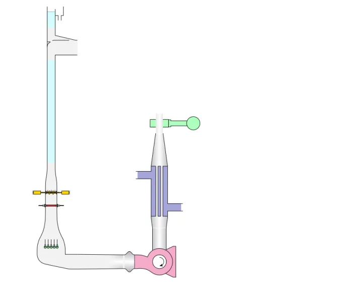
FIG. 1. Schematic of the Twente Mass and Heat Transfer Water Tunnel (TMHT). x, y, and z are the spanwise, wall-normal, and streamwise directions, respectively, where
each of the measurement sections has dimensions W (width), D (depth), and L (length) in the x, y, and z directions. (a) A side view cross section of the tunnel showing the major components. (b) The front and side profiles of the three exchangeable measurement sections and their respective contractions. (c) A top view of the active turbulent grid showing the 15 independently rotating rods with agitator flaps attached to them, here all in their horizontal position for displaying purposes. (d) The 12 cylindrical heater cartridges in red and the thermal insulation in yellow. (e) Bubble injection provided by five rows of each 28 exchangeable capillaries. The rows can be opened and closed independently from each other. See Sec.II Afor a walk-through description.
● A computer-controlled two-axis traversing frame allows for positioning sensors inside of the measurement section in order to obtain local quantities, such as the local tempera-ture by using thermistors with a few millikelvin resolution or the local gas volume fraction by using the optical fiber probe technique.25
● The local heat flux inside the flow can be measured by simultaneously acquiring local velocity with laser-Doppler anemometry and local temperature with a thermistor. In Secs.II A–II H, we will describe the TMHT facility in more detail.
A. Overview
We now give a quick walk-through of all the major components of the tunnel [seeFig. 1for a schematic picture andFig. 2(a)for a photo andFig. 2(b)for the coordinates system we have adopted]. Starting from the pump, the flow is expanded from a circular cross section to a larger rectangular area by the diffuser that has two later-ally adjustable vanes inside to help steer the flow sideways. The flow then enters the bend and is guided by three corner-turning vanes to facilitate uniformity in the downstream flow velocity profile.
A Pt100 temperature probe measures the bulk “inlet” liquid temperature. 140 exchangeable capillaries [detailed inFig. 1(e)] can
FIG. 2. (a) The Twente Mass and Heat Transfer Water Tunnel (TMHT) in the lab.
In the front (from bottom to top): the heaters, the active grid, and the measure-ment section. In the back (from top to bottom): settling vessel, flow meter, the heat exchanger, and the pump. (b) Sketch of the coordinate system and the dimensions of the measurement section.
inject bubbles into the flow near the bottom of this vertical tunnel section. Two modular sections follow that can be interchanged with each other. These are the section containing the heater cartridges [detailed inFig. 1(d)] and the section with the active turbulent grid [detailed inFig. 1(c)]. A contraction placed downstream of these sec-tions prevents the flow separation; it contracts the flow over its width (x-direction) and depth (y-direction).
Three interchangeable measurement sections of different cross sections can be installed. Their width and depth are either 0.3 × 0.04 m2, 0.3 × 0.06 m2, or 0.3 × 0.08 m2, each with a match-ing contraction of height 0.25 m [detailed inFig. 1(b)]. All those measurement sections are 1 m tall and their front, back, and one of the sides are made of glass. The remaining sidewall is of stainless steel and has equidistant portholes for inserting probes or inject-ing dye, and a wet/wet differential pressure transducer is attached to two of these portholes to monitor the gas volume fraction. The top part of the tunnel directly above the measurement section is open, and this can be used to insert a long probe holder, with, e.g., a thermistor attached to its end, down into the measurement section. The pole is attached to a computer-controlled two-axis traversing frame (not shown), allowing for automated positioning over thex and z-directions. The y-direction can be traversed manually by a positioning stage. At the top of the measurement section, the flow goes through a bend after which we find another Pt100 tempera-ture probe to register the bulk “outlet” liquid temperatempera-ture. Another Pt100 probe on the outside of the tunnel monitors the ambient air temperature of the lab. The flow then enters the settling vessel where
bubbles can rise up to the surface or where salt can be mixed into the liquid. Going downwards from the vessel, the flow is sped up by a funnel to pass through an electromagnetic flow rate meter. Finally, all heat that was added by the heater cartridges can be removed again by the pipe heat exchanger which is fed with a coolant from a chiller, after which the flow enters the pump again.
B. Flow control and adjustment
The flow in the tunnel is driven by a custom close-coupled axial flow propeller pump (Herborner Pumpenfabrik, Uniblock P 125-201/0074) fully cast from marine-grade AISI316 stainless steel to allow the use of saline solution. The capacity is 80 m3/h at a maximum power of 0.75 kW and 1500 rpm. The three-phase elec-tric motor of the pump is controlled by a digital frequency inverter (Herborner Pumpenfabrik, PED).
Directly after the pump is a rubber compensator to accommo-date for thermal expansion of the tunnel. A diffuser with a circular inlet with a diameter of 136 mm expands the flow to a rectangular outlet of 452 × 146 mm2. Inside the diffuser are two adjustable lat-eral vanes to help spread the flow sideways. The next bend directs the flow upwards. Inside the bend are three adjustable corner turning vanes that guide the flow and help increase flow velocity uniformity after the bend.
An electromagnetic flow meter (ABB, ProcessMaster FEP311) with a bore 65 mm measures the volumetric flow rate over its nom-inal range of 2.4 m3/h–120 m3/h. According to the manual, the measurement accuracy is better than 1% if the flow velocity through the meter is larger than 0.2 m/s, which is the reason for choosing this specific bore diameter. The flow is sped up by a funnel with an inclination angle of 8○before entering the meter.
The flow rate reported by the flow meter is continuously read out by an Arduino M0 Pro microcontroller board over a 4–20 mA current loop. A tuned proportional-integral controller programmed into the Arduino feeds back to the propeller rotation rate of the tun-nel pump over another 4–20 mA current loop to ensure a stable flow rate and velocity over time within 1% of the setpoint [seeFigs. 3(e)
and3(f)].
C. Temperature control and heat injection
Heat can be injected into the flow by 12 cylindrical heater cartridges (Watlow, Firerod J5F-15004) placed 300 mm below the measurement section and sticking perpendicular to the flow direc-tion through the front and back tunnel walls [seeFig. 1(d)]. Each heater cartridge has a diameter of 12.7 mm and a heated zone of 110 mm long as measured from its tip inside the tunnel, indi-cated by red. The end of the heated zone matches the start of the interior tunnel wall. Each heater is thermally insulated from the wall by a Teflon (PTFE, polytetrafluoroethylene) feed-through, indicated by yellow. A J-type thermocouple with an accuracy of ±2.2 K, for the absolute temperature, is embedded inside of each heater. Because the location of the thermocouple is not guaran-teed to be perfectly centered and a strong temperature gradient is to be expected in the interior of the heater cartridge when pow-ered and placed in a flow, the thermocouple temperature readings are only to be used as a rough indication of the heater temperature. Hence, they are solely used for over-temperature protection. The
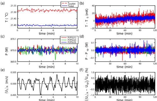
FIG. 3. Typical time series of the main global tunnel quantities after having settled to statistically stationary conditions, demonstrating the short-term fluctuations in
(a), (c), and (e) and the long-term stability in (b), (d), and (f). This specific case was at a set tunnel flow velocity of Usp= 0.5 m/s using measurement section #1
(subscript sp stand for setpoint), a chiller setpoint of 19○C, and a set heating power of 3 × 870 W = 2610 W divided over heaters 1–6. Heaters 1 and 2 were
con-nected in series to power supply PSU1, likewise 3 and 4 to PSU2 and 5 and 6 to PSU3. This caused the heaters to operate at an internal temperature of near 90○C. (a) Temperatures T of the tunnel inlet (solid blue) and outlet (dashed red). (b) The same data as the left panel, but with the starting temperature T
0subtracted.
The temperature drift is below 20 mK over 120 min. (c) Heating power P provided by power supplies PSU1 (red), PSU2 (green), and PSU3 (blue). (d) The same data as the left panel, but with the setpoint of the power Pspsubtracted. The power is stable within 0.15 W, regardless of the setpoint. (e) Instantaneous streamwise
flow velocity inside the measurement section ⟨Uz⟩Aaveraged over its cross-sectional area A (measured using the flow meter). The dashed line indicates the
set-point. (f) The same data as the left panel, but renormalized with the flow velocity setpoint Usp. The flow velocity is stable within 1% of the setpoint without drift over
120 min.
heaters are rated for temperatures in excess of 250○C, but will be limited by the over-temperature protection to a maximum of 95○C to prevent local boiling.
The heaters are operated by controlling the supply power. Each heater can provide 1160 W of heat at a maximum of 120 V. They are powered by three independently programmable DC power sup-plies (Keysight, N8741A), each providing up to 3.3 kW at 300 V and 11 A. Either a single heater is connected to a single power supply or multiple heaters are connected in series to a single power supply, and any combination of this depending on the needs of the experi-ment. The programming accuracy of the power supplies is 150 mV and 22 mA, and the measurement accuracy is 300 mV and 33 mA. A tuned proportional-integral controller running on a computer reg-ulates the power supply output voltage in order to tune the power output, resulting in an accuracy of the set power of ±0.3 W with a settling time of below 10 s. The power is stable within 0.15 W, regardless of the setpoint [seeFigs. 3(c)and3(d)].
The bulk temperature of the liquid inside the tunnel is mea-sured at two locations using two Pt100 temperature probes with a 1/10 DIN accuracy corresponding to ±30 mK (Pico Technology, PT-104 data logger with SE012 probes). One probe labeled “inlet” is upstream of the heaters at the location of the bubble injectors and protrudes 100 mm into the flow [see Fig. 1(a)]. The other probe
labeled “outlet” is downstream of the measurement section and in front of the settling vessel. A third Pt100 probe labeled “ambient” measures the ambient lab air temperature.
Cooling of the tunnel liquid is taken care of by a pipe heat exchanger, manufactured on request by Geurts International, located just in front of the tunnel pump intake. Twenty-two marine-grade AISI316 stainless steel pipes of 500 mm long and with diam-eters of 22 mm through which the tunnel liquid is flowing are embedded in an outer jacket through which cooling water is flow-ing. The pipe heat exchanger is designed to remove up to 10 kW of heat. The temperature of the cooling water is regulated by a 12.5 kW capacity air-cooled recirculating chiller (Thermo Sci-entific, ThermoFlex 15000 P5) with a listed temperature stability of ±0.1 K.
We will now show a typical example of settling times and tem-perature stability. Starting with a quiescent water-filled tunnel at room temperature, it takes up to 2.5 h to settle to a statistically sta-tionary state, from the moment of setting the flow rate to 21.6 m3/h (equivalent to a velocity of 0.5 m/s in the measurement section #1), the global heat input to 2.6 kW, and the setpoint of the chiller at 19○C. After this settling time, we report a long-term stability of the tunnel liquid temperature of less than ±10 mK for a duration of over 2 h (seeFig. 3).
D. Local temperature measurements
High precision and local temperature measurements can be made with thermistors. We use thermistors from TE Connectiv-ity (Measurement Specialties G22K7MCD419) with a glass bead of diameterd = 0.38 mm and a listed response time of 30 ms in liquids. The temperature response time can also be estimated by consider-ing the temperature inside the glass bead, and the temperature “skin thickness” is given by δ = √αt. For a penetration of δ = 0.4d, we findt = 29 ms, which is in accordance with the listed temperature response. All thermistors are calibrated against the “inlet” Pt100 probe with a 1/10 DIN accuracy, corresponding to ±30 mK (Pico Technology, PT-104 data logger with SE012 probe) inside of a large copper body placed in a temperature bath with a 5 mK temperature stability (PolyScience, PD15R-30), resulting in a calibration accuracy of ±30 mK and a 5 mK resolution.
Temperature time series can be acquired by using a dual-phase lock-in amplifier (Stanford Research, SR830) in combination with a balanced Wheatstone bridge of which one arm is a single ther-mistor. A digital acquisition card (National Instruments, PCI-6221) logs the amplifier’s output voltage to a file on the computer. Mul-tiple thermistors can be logged during a measurement by a digital multimeter (Keysight, 34972A) installed with a reed-relay multi-plexer board (Keysight, 34902A) that will scan sequentially over all the thermistor resistance values with a listed scan rate of up to 250 channels/s.
E. Traverse
Accurately positioning thermistors, optical fibers, or other probes inside of the measurement section and automatically scan-ning over multiple grid points are made possible by a custom-built two-axis traversing frame located above the tunnel. The tra-verse consists of two linear actuators (Parker, HMRB15SBD0-1800 and HMRB11SBD0-1000), powered by two servomotors (Parker, SMHA60451 and SMH60301) and digitally operated by two con-trollers (Parker, Compax3). The traverse can travel over the full width (x-direction) and full height (z-direction) of the measure-ment section. A probe holder is attached to the traverse carriage and descents into the measurement section from an opening in the top of the tunnel. The carriage can be positioned with an accuracy of ±0.1 mm. The third axis (depth, y-direction) can be traversed over manually by using the microstage that is in between the traverse carriage and the traverse pole.
F. Bubble injection and gas volume fraction
Bubbles can be injected into the flow by the pressurized air lines that are fed through the wall of the tunnel located underneath the heater cartridges. The lines are pressurized at 8 bars and connected to five rows of 28 Luer lock fittings [seeFigs. 1(a)and1(e)]. The stan-dardized Luer lock allows for a wide variety of needles/capillaries to be installed and easily replaced (e.g., Nordson precision stainless steel dispensing tips), ranging from inner diameters of 0.2 mm to 2 mm. The resulting size of the bubbles detaching from the capillar-ies may be influenced by the local velocity and shear of the surround-ing liquid, surfactants, air flow rate, and the geometry of the tip of the capillaries. Each of the five rows can be opened or closed individually by computer controlled piston valves. A digital mass flow controller
(Bronkhorst, F-111AC-50K-AAD-22-V) drives air through all five rows at up to 44 l/min.
The global gas volume fraction over the full height of the mea-surement section is monitored by a wet/wet differential pressure transducer (Omega, PXM409170HDWUI). The pressure transducer is connected to two portholes, with a distance of ΔL = 0.96 m in height apart, at the side of the measurement section. Each of these portholes has just a narrow channel of 1.0 mm in diame-ter that connects to the tunnel’s indiame-ternal volume. This ensures that no air will enter the lines from the portholes toward the pressure transducer and that they are always filled with liquid. The result-ing difference in static pressure between these lines and the liquid column inside the measurement section translates into the relation α =ΔP/(gρlΔL), where α is the global gas volume fraction over the measurement section, ΔP is the measured pressure difference, g is the local acceleration of gravity, ρlis the density of the liquid, and ΔL is the distance in height between the portholes. We report a constant measurement accuracy in α of ±0.2%, given already in units of the gas volume fraction percentage. Injecting 36 l/min of air through the bubble injection capillaries, we can achieve a maximum of α = 7.8% ± 0.2% when the tunnel pump is switched off, and, e.g., α = 5.3% ± 0.2% at a flow velocity of 0.5 m/s inside measurement section #1.
The local gas volume fraction, bubble size, and bubble veloc-ity statistics can be obtained by the optical fiber probe technique. For details on this experimental technique and signal processing, we refer to Cartellier25and van Gilset al.26
G. Active turbulent grid
The active turbulent grid consists of 15 independently rotat-ing rods with agitator flaps attached to them that stir up the liquid flowing past [seeFigs. 1(a)and1(c)]. It resembles the grid described in Sec. 3.3.1 of Poorte and Biesheuvel,27 albeit with modern DC-motors (Maxon, DCX32L GB KL 24V) and controllers (Beckhoff, EL7332) and with only 15 rods instead of 24 because of the smaller cross-sectional area of the tunnel. There are several forcing protocols that can be used to drive the rods independently at varying rota-tion speeds and direcrota-tions for varying periods of time. The study over the different protocols by Poorte and Biesheuvel27revealed that
thedouble-random asynchronous mode protocol is the most favor-able, as this protocol does not lead to periodicities in the turbulent power spectrum directly downstream of the grid. Hence, this proto-col (P0238) is the standard we use in our studies. In short, it varies the rotation speed of a single rod and the duration of that rotation by randomly choosing values from the intervals [−Ωm, Ωm] and [50, 90] ms, respectively. A control parameter called “grid speed factor” GSF will rescale the value of Ωmsuch that the amount of agitation can be tailored. For example, the nominal value of Ωmat a grid speed factor of 0.5 corresponds to 18 Hz.
H. System control
The system control of the TMHT facility is controlled by two programmable multifunction microcontroller boards in conjunc-tion with a personal computer (PC) [seeFig. 4for a simplified dia-gram]. The boards used are two Arduino M0 Pro which are powered by a SAMD21 microcontroller unit from Atmel, featuring a 32-bit ARM Cortex M0 core.
FIG. 4. System control diagram. The tunnel filling system and water level monitoring running on Arduino #2 are not discussed in this work and are mentioned for completeness.
One major source of electrical noise is carried by the lab facil-ity electrical ground. Inductive spikes induced by, e.g., motors or switching relays can travel over the ground leads and can inter-fere with the sensitive microcontrollers. To prevent ground loops, ground noise, or inductive spikes from reaching the sensitive micro-controllers, one has to float the microcontroller board with respect to the lab facility ground potential. We do this by powering the micro-controllers using a noise-suppressing power supply (Traco Power, TCL 120-112) whose output is left floating with respect to ground. That means that ground-referenced peripheral devices cannot be connected to the Arduino directly, lest we lose the floating ground reference. Hence, all universal serial bus (USB) connections from the microcontrollers to the PC are galvanically isolated by USB iso-lators (Olimex, USB-ISO). All peripheral digital sensors and actu-ators are connected to the microcontrollers with optocouplers in between.
All analog signals from and to the microcontrollers (i.e., set pump speed, flow meter, and read pressure transducer) transmit over 4–20 mA current loops, which are inherently insensitive to electrical noise in contrast to using voltage as a data carrier. The 4–20 mA current transmitter and receivers used are MIKROE-1296 T Click and MIKROE-1387 R Click from MikroElektronika, respec-tively. The remaining peripheral devices (i.e., the Pt100 data log-ger, programmable power supplies, digital multimeter multiplex-ers, mass flow controller, active turbulent grid, chiller, and traverse controllers) are directly connected to the PC.
The main control program is running in Python 3.6 on the PC and handles all device input/output communication includ-ing the microcontrollers, with the exception of the active turbulent grid which is running on LabView from National Instruments. The main program has a graphical user interface to provide control,
monitoring, and data logging of the TMHT facility, whose global quantities are logged at a rate of 10 Hz. The Python libraries that have been written to provide multithreaded communication with the specific laboratory devices including the Arduino microcontrollers are made available under the MIT open-source license and can be found at the GitHub repository.28
III. EXAMPLES OF FLOW AND TEMPERATURE MEASUREMENTS
A. Velocity profile measurements
The transparent measurement section of the THMT allows for the measurements of the local velocity using a variety of optical tech-niques including particle image velocimetry (PIV), laser Doppler anemometry (LDA), and particle tracking velocimetry (PTV), which could even be performed simultaneously if needed. As a first step in demonstrating the robustness and consistency of the setup, we measure the liquid velocity using two experimental techniques: LDA in backscatter mode and PIV in measurement section #1 (width × depth: 0.3 × 0.04 m2). For LDA measurements, the flow is seeded with polyamide seeding particles (diameter 5 μm and den-sity 1050 kg/m3). The LDA system used consists of DopplerPower DPSS (diode-pumped solid-state) laser and a Dantec burst spectrum analyzer (BSA). For PIV, we seed the flow with fluorescent tracer particles (diameter 50 μm). We use a high speed laser (Litron LDY-303HE) with a cylindrical lens to generate a sheet of light passing through the center of the glass side-wall of the measurement sec-tion (y/D = 0.5). A double-frame camera (PCO Imager sCMOS) at 20 fps was used to obtain the velocity field. All the velocity pro-files obtained using PIV presented in this section are calculated by
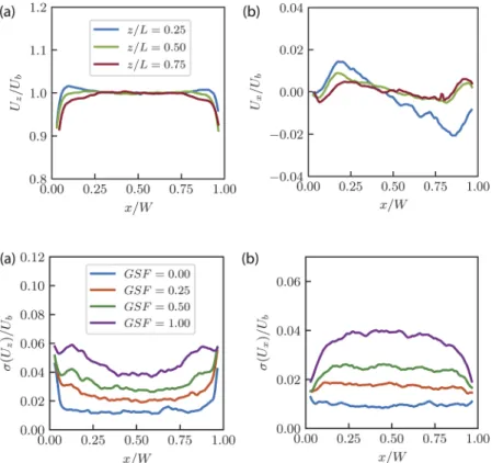
FIG. 5. Normalized (a) streamwise Uz and (b) spanwise
Ux velocity profiles along the width of the setup at
half-height obtained from PIV measurements for different mean flow rates ⟨Uz⟩Aand constant speed of the active grid (the
active grid is running at GSF = 0.5). Ubis the streamwise
velocity in the bulk, calculated by averaging the measured velocity over the width x/W = 0.25 to x/W = 0.75.
averaging the velocity over several heights, covering ±5 cm around the noted height.
InFigs. 5(a)and5(b), we plot the normalized mean profile of the streamwise and spanwise velocity obtained from PIV measure-ments for different mean flow rates, namely, 0.3 m/s, 0.5 m/s, 0.8 m/s, and 1.0 m/s, for a constant active grid speed factor of 0.5. We find that the variation of the mean horizontal and vertical veloc-ity is negligible in the bulk of the setup, namely, not more than ±1.5% from the mean streamwise velocity. InFig. 5(b), we see that the span-wise velocity has a positive and negative peak, which is a signature of the contraction section placed downstream of the measurement section.
Next, we look at the velocity profiles for ⟨Uz⟩A= 0.5 m/s and GSF = 0.5 at different heights, namely, at z/L = 0.25, z/L = 0.5, and
z/L = 0.75. InFig. 6(a), we see that the streamwise velocity remains constant (within ±2%) along the width at different heights. By scan-ning the velocity at different heights, we observe that the influence of the contraction on the spanwise velocity reduces as the height increases, although its amplitude is only of the order of 1% of the streamwise component [seeFig. 6(b)].
InFig. 7, we plot the turbulence intensity measured using PIV at half-height for ⟨Uz⟩A = 0.5 m/s and study the influence of the active grid on the velocity statistics. By varying the grid speed fac-tor (GSF) from 0 to 1, it is easily observed that the active grid has a strong influence on the velocity fluctuations. For a grid speed factor (GSF) equal to zero, the active grid is switched off and the rods are placed in such a way that the flaps are open, forming a passive grid instead. In this case, we observe the weakest velocity fluctuations.
FIG. 6. Normalized (a) streamwise Uzand (b) spanwise Ux
velocity profiles along the width of the setup obtained from PIV measurements at different heights for mean flow rate of ⟨Uz⟩A=0.5 m/s and constant speed of the active grid
GSF = 0.5. Ubis the streamwise velocity in the bulk at each
height, calculated by averaging the measured velocity over the width x/W = 0.25 to x/W = 0.75.
FIG. 7. Turbulence intensity in (a) streamwise and (b)
span-wise directions along the width of the measurement sec-tion at half-height obtained from PIV measurements for ⟨Uz⟩A = 0.5 m/s and varying speed of rotation of the active grid [varying the value of the grid speed factor (GSF)].
GSF = 0 corresponds to the measurement with the active
grid switched off, while for GSF = 1, rods are rotating at a maximum speed.σ(Uz) is the standard deviation of the
streamwise velocity, whileσ(Ux) is the standard deviation
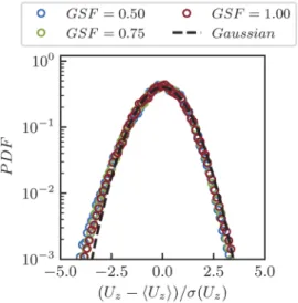
FIG. 8. Probability density function of the streamwise velocity for ⟨Uz⟩A=0.5 m/s and different values of the grid speed factor, obtained at x/W = 0.5, y/D = 0.5, and
z/L = 0.5 using LDA. Gaussian with zero mean and unit variance is added for
reference.
As the GSF increases, the fluctuations increase up to 3 times, and for each of the cases, the velocity fluctuations remain nearly constant along the width in the bulk. InFig. 8, we show the probability den-sity function (PDF) of the streamwise velocity obtained from LDA measurements for different GSFs at the center of the setup (x/W = 0.5, y/D = 0.5, and z/L = 0.5) at a mean flow rate of 0.5 m/s. We observe that for all the settings of the active grid, the distri-bution of the vertical velocity nearly follows a normal distridistri-bution, with a skewness of around 0.2 and a kurtosis of around 3.25 for all cases.
Furthermore, we examine the homogeneity in the wall-normal direction by measuring the vertical velocity along the depth of the setup atz/L = 0.5, ⟨Uz⟩A = 0.5 m/s, and GSF = 0.5 using LDA and PIV measurements. The results presented inFig. 9demonstrate that the velocity is nearly constant in the wall-normal direction as well,
FIG. 9. LDA-scan and PIV measurement of the vertical velocity along the depth
of the setup at half-height performed for ⟨Uz⟩A=0.5 m/s and GSF = 0.5. The bars for the LDA correspond to ±1 standard deviation of the velocity. Dashed lines presentδ99for both boundary layers.
FIG. 10. Scan of the vertical velocity along the width of the setup at half-height
performed using LDA and PIV for ⟨Uz⟩A = 0.5 m/s and GSF = 0. The bars corresponds to ±1 standard deviation of the velocity. The bars correspond to ±1 standard deviation of the velocity.
with variations of only around ±2% fromy/D = 0.2 to y/D = 0.8. Furthermore, we identify the boundary layer thicknesses by the δ99 criterium and find that δ99= 0.28D on the left and δ99= 0.30D on the right, leaving a large center flow of ≈0.4D outside the boundary layers.
Finally, we compare PIV and LDA measurements of the streamwise velocity profiles inFig. 10. We find very good overlap within 1%–2%. Note that these were not measured simultaneously but on different moments, which could explain the slight differ-ence between them. The advantage of the PIV measurements is that an entire field is measured at once, rather than measuring point-by-point (LDA). The downside is the difficulty of using PIV in two-phase flows, which is possible with LDA for low volume frac-tions α. Another advantage of LDA over PIV is that the processing requirements are orders of magnitude less for LDA measurements as compared to PIV measurements. LDA also easily offers very high data-rates, which can be tricky for PIV due to the requirements of lasers and cameras.
B. Local temperature measurements
Here, we examine the influence of heating of one half of the heating section on the temperature profile in the measurement sec-tion of dimensions width × depth = 0.3 × 0.04 m2, with the mean liquid flow of 0.5 m/s and the grid speed factor of 0.5. In this spe-cific configuration, six heaters (out of 12 total) which are placed in the left half (x/W ≤ 0.5) of the heating section have been sup-plied by a constant power of 870 W each. The thermistor for the temperature measurements is inserted to the measurement sec-tion from the sidewall of the secsec-tion and traversed over the width at half height. The measurements are logged at 2 Hz by a digi-tal multimeter over 2 h after a statistically steady state is achieved.
Figure 11 shows the temperature profile obtained in such a way, where heating was introduced in the heating section x/W ≤ 0.5. Here, ΔT = Tinlet− T is the difference between the temperature mea-sured before the heatersTinletand the temperature measured in the bulk in the measurement sectionT. We observe a decrease in ΔT fromx/W = 0 to x/W = 1 as a consequence of heating of only one half of the section.
FIG. 11. Temperature profile at half height in the case of heating of the left half x/W = 0 to x/W = 0.5 of the setup. Here,ΔT = T − Tinlet, where Tinletis the inlet
temperature measured before the heaters and T is the temperature measured by a thermistor in the measurement section.
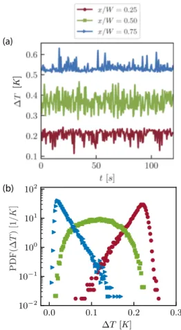
FIG. 12. (a) Temperature series measured at different locations: x/W = 0.25 above
the heated area, x/W = 0.50 in the center of the setup, and x/W = 0.75 above the nonheated area. Note that for the signals at x/W = 0.50 and x/W = 0.75, offsets of 0.25 K and 0.50 K, respectively, are applied, for clarity of reading the figure. (b) Probability density function of the temperature at different locations of the setup:
x/W = 0.25 above the heated area, x/W = 0.50 in the center of the setup, and x/W = 0.75 above the nonheated area.
After passing the heated section, warm and cold volume of liquid mix, resulting in different temperature signals in the mea-surement section atx/W = 0.25, x/W = 0.5, and x/W = 0.75 [see
Fig. 12(a)]. This is also reflected on the probability density func-tion shown inFig. 12(b). Namely, negative skewness is observed for the signal atx/W = 0.25 due to nonheated liquid penetrating to the opposite side of the section. In the center (x/W = 0.5), where the mixing between cold and warm part of the bulk is the most intense, the signal is not skewed (skewness = 0), i.e., positive and negative fluctuations are equally represented. Again atx/W = 0.75, warm liq-uid parcels penetrate the cold part of the bulk, yielding a positively skewed PDF.
C. Combined velocity and temperature measurements
To measure the local heat flux, we need to simultaneously measure the temperature and local velocity at the same position
FIG. 13. Combined velocity and temperature measurements at the middle of the
tunnel (x/W = y/D = z/L = 0.5) with mean liquid velocity ⟨Uz⟩A =0.5 m/s, the active grid speed factor GSF = 0.5, and the total heating power 2.25 kW for heaters 1–6. (a) Standardized (zero mean, unit variance) probability density function of the temperature. For reference, we have added a normal distribution with zero mean and unit variance as a black dashed line. (b) Standardized probability density function of the velocitiesv˜i= (vi− ⟨vi⟩)/σ(vi), where i = x is the horizontal
direction and i = z is the vertical direction. (c) Standardized probability density function of the product of the velocity and the temperature fluctuations (T′=T
in the flow. We measure the local temperature using a thermistor that is connected to one arm of a Wheatstone bridge so that very small variations of the resistance of the thermistor can be measured. We utilize a lock-in amplifier (SRS SR830) in order to reduce noise. We place the thermistor in the middle of the measurement section. We position the measurement volume of our LDA configuration just upstream ≈0.5 mm of the thermistor. We synchronize the two sys-tems and for a flow velocity of ⟨Uz⟩A = 0.5, an active grid speed factorGSF = 0.5, and heat injection by heaters 1–6 with a total of 2.25 kW, we measured the local temperature and the flow velocity (seeFig. 13). We find that the horizontal velocity vx and the tem-perature fluctuations (T′ = T − ⟨T⟩) are strongly correlated with a Pearson correlation coefficient of ρvx,T′ ≈ 0.37, while we find that
the vertical velocity and the temperature are not correlated at all ρvz,T′≈ 0.00. This results in a positively skewed temperature
proba-bility density function for ˜Jxwith broad thick tails (kurtosisK = 7.5) but not for ˜Jz, where we find a platykurtic distribution (K = 2.6), akin to the distribution of the temperature itself.
D. Dispersion of a passive scalar in a turbulent bubbly flow
The TMHT offers the possibility of studying the mixing of a passive scalar in turbulent bubbly flow. The primary advantage of this setup over, for example, the Twente Water Tunnel29 is that in this setup we can easily achieve gas volume fractions higher than 1%. For the purpose of studying mixing of a low-diffusive dye induced by a swarm of high Reynolds number bubbles rising within a turbulent flow, we inject a fluorescent dye (fluorescein sodium) in the tunnel with measurement section #2 (width × depth = 0.3 × 0.06 m2
). The dye injector (diameter 2 mm) is placed in the middle of the cross section 20 cm away from the bottom of the measure-ment section. The injection is performed over 60 s at a flow rate matching the mean liquid velocity in the tunnel (∼30 cm/s). The images of the flow are taken 10 s after the start of the injection, using two synchronized and vertically aligned cameras (Imager sCMOS,
Lavision) with 105 mm macrolenses and optical bandpass filters (450–650 nm).
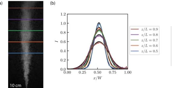
InFig. 14(a), we show an instantaneous snapshot of the fluo-rescent dye being advected and diffused in the presence of a bubbly turbulent flow. Using a time series of such snapshots, we measure the mean intensity profiles of the fluorescent lightI across the width of the setup at different heights; profiles for a few selected heights are shown inFig. 14(b). The profiles are symmetric due to the homo-geneity of the flow in the horizontal direction. Additionally, we find that the profiles are nearly normally distributed, suggesting that the spreading of the dye in the horizontal dimension is dominated by diffusion. The objective of future studies is to obtain the horizon-tal diffusion coefficient by measuring concentration of the dye by means of quantitative laser induced fluorescence. For further details on this experimental technique, we refer to Alméraset al.30 E. Salt
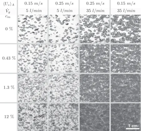
As discussed in Sec. I, the TMHT also allows the possibil-ity to study the dynamics of bubbles injected in brine (salt solu-tion). We perform preliminary tests by varying the mean liquid flow rate, the gas flow rate, and the concentration of salt (NaCl) in the brine solution with a constant grid speed factorGSF = 0.4, while using measurement section #2. InFig. 15, we show snapshots for the different cases. Images were taken using a Photron SA1 camera at 1000 fps.
We visually observe a big difference in the flow regimes as we increase the salt concentration of the solution fromcm= 0% to cm= 12% (mass fraction). The effect is more pronounced when the gas flow rate is higher, which may be due to the presence of more smaller bubbles caused by the increase in surface tension by the addi-tion of salt. This also leads to a reducaddi-tion in the deformability of the bubbles and consequently to a change in the dynamics of the system.
By means of image processing, we measure the bubble diam-eter for the cases of mean liquid velocity 0.15 m/s and 0.25 m/s
FIG. 14. Dispersion of a fluorescent dye
in a bubbly turbulent flow with ⟨Uz⟩A
=0.30 m/s. (a) Instantaneous snapshot of the flow taken at an arbitrary time showing the spatial distribution of the flu-oresced light. (b) Time averaged light intensity profiles across the width of the setup at different heights (in color) and corresponding Gaussian fits.
FIG. 15. Snapshots of the flow in the TMHT with the
addi-tion of increasing salt concentraaddi-tion (from top to bottom), for various water flows and gas flow rates. ⟨Uz⟩Ais the mean
liquid streamwise velocity, ˙Vgis the gas flow rate, and cmis
the mass fraction of salt in the solution.
and a gas flow rate of 5 l/min for varying salt concentrations. In
Figs. 16(a)and16(b), we show sample images from two different simple image processing algorithms for edge detection implemented using Matlab. For cases with low concentrations of salt (cm≤ 1.3%), we identify contours of objects as well as boundaries of holes inside these objects [seeFig. 16(a)]. The criterium used to identify bub-bles is that the area of the outermost object is 1.3 times greater than the area of the object completely enclosed by it. For the case of high salt concentrationcm= 12%, for which more spherical bubbles are present, bubbles are selected by identifying round objects under the condition that the bubbles are in focus [seeFig. 16(b)]. Each method
detects at least 1300 bubbles for each of the examined cases. The distributions of the equivalent bubble diameter for 4 concentrations and 2 flow speeds are shown inFig. 16(c). Note that the bubble size is determined from the images taken from the side which causes a large spread in the volume-determination as the information of the depth is lacking and the shape of the bubble constantly changes as the bubble deforms while rising. We find that a small increase in the concentration of salt fromcm= 0% tocm = 1.3% significantly decreases the average bubble diameter. Further increasing the salt concentration fromcm= 1.3% tocm= 12% seems to have hardly any influence on the average bubble diameter. For each examined salt
FIG. 16. (a) Zoomed-in view of a snapshot for the case of mean liquid velocity ⟨Uz⟩A=0.15 m/s, gas flow rate ˙V = 5 l/min, and cm= 0%, showing bubbles identified as
pairs of objects. (b) Zoomed-in view of a snapshot for the case of ⟨Uz⟩A=0.15 m/s, gas flow rate ˙V = 5 l/min, and cm= 12%, showing bubbles identified as round objects.
(c) Distribution of the bubble diameter for ⟨Uz⟩A=0.15 m/s and ⟨Uz⟩A=0.25 m/s for varying salt concentrations. The mean values of the diameter are indicated using points.
concentration, an increase in the mean liquid flow rate resulted in almost no change in the average bubble diameter. Future studies in this setup will be dedicated to studying the effect of salt on the dynamics of the system and the coupling of heat transport with the salt concentration.
IV. SUMMARY AND OUTLOOK
A new experimental facility the Twente Mass and Heat Trans-fer Water Tunnel (TMHT) has been built. This facility has global temperature control, bubble injection, and local heat/mass injec-tion and offers the possibility to study heat and mass transfer in turbulent multiphase flow. The tunnel is made of high-grade stain-less steel permitting the use of salt solutions in excess of 15% mass fraction, besides water. The total tunnel volume is 300 l. Three inter-changeable measurement sections of 1 m height but of different cross sections (0.3 × 0.04 m2, 0.3 × 0.06 m2, and 0.3 × 0.08 m2) span a Reynolds-number range from 1.5 × 10⁴ to 3 × 10⁵ in the case of water at room temperature. The glass vertical measurement sec-tions allow for optical access to the flow, enabling techniques such as laser Doppler anemometry, particle image velocimetry, particle tracking velocimetry, and laser-induced fluorescent imaging. Ther-mistors mounted on a built-in traverse provide local temperature information at a few millikelvin accuracy. Combined with simulta-neous local velocity measurements, the local heat flux in single phase and two phase turbulent flow can be studied.
We demonstrated long term and short term stability of the power of the heaters and the cooler, of the inlet and outlet temper-ature of the tunnel, and the mean flow rate. PIV and LDA measure-ments were performed for a variety of flow conditions to show that homogeneity of the flow is satisfying. Preliminary temperature mea-surements in single phase flow and meamea-surements with salt and dye injection in two phase flows were performed as well.
ACKNOWLEDGMENTS
This work was part of the Industrial Partnership Programme i36 Dense Bubbly Flows that was carried out under an agreement between AkzoNobel (Nouryon since October 2018), DSM Innova-tion Center B.V., SABIC Global Technologies B.V., Shell Global Solutions B.V., TATA Steel Nederland Technology B.V., and the Netherlands Organisation for Scientific Research (NWO). Chao Sun acknowledges the financial support from the Natural Science Foun-dation of China under Grant No. 11672156. This work was also sup-ported by The Netherlands Center for Multiscale Catalytic Energy Conversion (MCEC), an NWO Gravitation Programme funded by the Ministry of Education, Culture and Science of the Government of The Netherlands. The authors thank Bert Vreman for his contri-butions to the measurements with salt, Varghese Mathai for fruitful discussions and useful insights, Rodrigo Ezeta for helping set up the PIV measurements, and Bas Dijkhuis and Hein-Dirk Smit for participating in the velocity and temperature measurements. REFERENCES
1R. F. Mudde, “Gravity-driven bubbly flows,”Annu. Rev. Fluid Mech.
37, 393–423 (2005).
2F. Risso, “Agitation, mixing, and transfers induced by bubbles,”Annu. Rev. Fluid
Mech.50, 25–48 (2018).
3
N. Deen, R. Mudde, J. Kuipers, P. Zehner, and M. Kraume, “Bubble columns,” in Ullmann’s Encyclopedia of Industrial Chemistry (Wiley-VCH Verlag, 2010).
4D. Darmana, N. G. Deen, and J. A. M. Kuipers, “Detailed 3D modeling of
mass transfer processes in two-phase flows with dynamic interfaces,”Chem. Eng. Technol.29, 1027–1033 (2006).
5D. Jain, Y. M. Lau, J. Kuipers, and N. G. Deen, “Discrete bubble modeling for
a micro-structured bubble column,” in11th International Conference on Gas-Liquid and Gas-Gas-Liquid-Solid Reactor Engineering [Chem. Eng. Sci.100, 496–505 (2013)].
6
G. Besagni, F. Inzoli, and T. Ziegenhein, “Two-phase bubble columns: A com-prehensive review,”ChemEngineering2, 13 (2018).
7W.-D. Deckwer, “On the mechanism of heat transfer in bubble column reactors,”
Chem. Eng. Sci.35, 1341–1346 (1980).
8
J. Heijnen and K. V. Riet, “Mass transfer, mixing and heat transfer phe-nomena in low viscosity bubble column reactors,”Chem. Eng. J.28, B21–B42 (1984).
9
A. A. Kulkarni, “Mass transfer in bubble column reactors: Effect of bubble size distribution,”Ind. Eng. Chem. Res.46, 2205–2211 (2007).
10A. Kitagawa and Y. Murai, “Natural convection heat transfer from a vertical
heated plate in water with microbubble injection,”Chem. Eng. Sci.99, 215–224 (2013).
11D. Colombet, D. Legendre, F. Risso, A. Cockx, and P. Guiraud, “Dynamics
and mass transfer of rising bubbles in a homogenous swarm at large gas volume fraction,”J. Fluid Mech.763, 254–285 (2015).
12A. T. Tokuhiro and P. S. Lykoudis, “Natural convection heat transfer from a
vertical plate—I. Enhancement with gas injection,”Int. J. Heat Mass Transfer37, 997–1003 (1994).
13H. Ayed, J. Chahed, and V. Roig, “Hydrodynamics and mass
trans-fer in a turbulent buoyant bubbly shear layer,” AIChE J. 53, 2742–2753 (2007).
14N. G. Deen and J. A. M. Kuipers, “Direct numerical simulation of wall-to
liq-uid heat transfer in dispersed gas-liqliq-uid two-phase flow using a volume of flliq-uid approach,”Chem. Eng. Sci.102, 268–282 (2013).
15S. Dabiri and G. Tryggvason, “Heat transfer in turbulent bubbly flow in vertical
channels,”Chem. Eng. Sci.122, 106–113 (2015).
16
B. Gvozdi´c, E. Alméras, V. Mathai, X. Zhu, D. P. van Gils, R. Verzicco, S. G. Huisman, C. Sun, and D. Lohse, “Experimental investigation of heat trans-port in homogeneous bubbly flow,”J. Fluid Mech.845, 226–244 (2018).
17
B. Gvozdi´c, O.-Y. Dung, E. Alméras, D. P. van Gils, D. Lohse, S. G. Huisman, and C. Sun, “Experimental investigation of heat transport in inhomogeneous bubbly flow,”Chem. Eng. Sci.198, 260 (2018).
18
A. Kitagawa, K. Kosuge, K. Uchida, and Y. Hagiwara, “Heat transfer enhance-ment for laminar natural convection along a vertical plate due to sub-millimeter-bubble injection,”Exp. Fluids45, 473–484 (2008).
19
K. Sekoguchi, M. Nakazatomi, and O. Tanaka, “Forced convective heat transfer in vertical air-water bubble flow,” Bull. JSME 23, 1625–1631 (1980).
20
Y. Sato, M. Sadatomi, and K. Sekoguchi, “Momentum and heat transfer in two-phase bubble flow—I. Theory,” Int. J. Multiphase Flow 7, 167–177 (1981).
21
Y. Sato, M. Sadatomi, and K. Sekoguchi, “Momentum and heat transfer in two-phase bubble flow—II. A comparison between experimental data and theoretical calculations,”Int. J. Multiphase Flow7, 179–190 (1981).
22
A. Kitagawa, K. Uchida, and Y. Hagiwara, “Effects of bubble size on heat transfer enhancement by sub-millimeter bubbles for laminar natural convection along a vertical plate,”Int. J. Heat Fluid Flow30, 778–788 (2009).
23
A. Kitagawa, K. Kimura, and Y. Hagiwara, “Experimental investigation of water laminar mixed-convection flow with sub-millimeter bubbles in a vertical channel,”
Exp. Fluids48, 509–519 (2010).
24
P. T. Nguyen, M. A. Hampton, A. V. Nguyen, and G. R. Birkett, “The influ-ence of gas velocity, salt type and concentration on transition concentration for bubble coalescence inhibition and gas holdup,”Chem. Eng. Res. Des.90, 33–39 (2012).
25A. Cartellier, “Optical probes for local void fraction measurements:
26
D. P. M. van Gils, D. Narezo Guzman, C. Sun, and D. Lohse, “The importance of bubble deformability for strong drag reduction in bubbly turbulent Taylor–Couette flow,” J. Fluid Mech. 722, 317–347 (2013).
27
R. Poorte and A. Biesheuvel, “Experiments on the motion of gas bub-bles in turbulence generated by an active grid,” J. Fluid Mech. 461, 127 (2002).
28
D. P. M. van Gils, Python library for (multithreaded) communication with laboratory instruments, University of Twente, 2018, https://github.com/Dennis-van-Gils.
29
R. Poorte, “On the motion of bubbles in active grid generated turbulent flows,” Ph.D. thesis, Universiteit Twente, 1998.
30E. Alméras, F. Risso, V. Roig, S. Cazin, C. Plais, and F. Augier, “Mixing by