Topology optimization of heat and mass transfer in bi-fluid laminar flow : application to heat exchangers

HAL Id: tel-02274990

https://pastel.archives-ouvertes.fr/tel-02274990

HAL is a multi-disciplinary open access archive for the deposit and dissemination of sci-entific research documents, whether they are pub-lished or not. The documents may come from teaching and research institutions in France or abroad, or from public or private research centers.

L’archive ouverte pluridisciplinaire HAL, est destinée au dépôt et à la diffusion de documents scientifiques de niveau recherche, publiés ou non, émanant des établissements d’enseignement et de recherche français ou étrangers, des laboratoires publics ou privés.

Topology optimization of heat and mass transfer in

bi-fluid laminar flow : application to heat exchangers

Rony Tawk

To cite this version:

Rony Tawk. Topology optimization of heat and mass transfer in bi-fluid laminar flow : application to heat exchangers. Thermics [physics.class-ph]. Université Paris sciences et lettres, 2018. English. �NNT : 2018PSLEM017�. �tel-02274990�

THÈSE DE DOCTORAT

de l’Université de recherche Paris Sciences et Lettres 

PSL Research University

Préparée à MINES ParisTech

Topology optimization of heat and mass transfer in bi-fluid laminar flow:

application to heat exchangers

Optimisation topologique des transferts de masse et de chaleur en écoulement

bi-fluide laminaire : application aux échangeurs de chaleur

COMPOSITION DU JURY :

Mme.

Alicia

ENSMA, Rapporteur, Président  Mme Marie-Christine DULUC LIMSI, Membre du jury

M. Yannick PRIVAT UPMC, Membre du jury M. Dominique MARCHIO

Mines ParisTech, Membre du jury

Soutenue par Rony

TAWK

Le 19 juin 2018

h

Ecole doctorale

n°432

SCIENCES DES METIERS DE L’INGENIEUR

Spécialité

ENERGETIQUE ET PROCEDES

Dirigée par Dominique MARCHIO

ii

When you work you are a flute through whose heart the whispering of the hours turns to music.

iii

Acknowledgments

This thesis would not have been possible without the support and guidance of many people who contributed in the preparation and completion of the work.

Firstly, I would like to express my very great appreciation to my advisor Dr. Maroun Nemer for the continuous support of my PhD study and related research, for his motivation, and immense knowledge. His very constructive criticism has contributed immensely to the evolution of my ideas on the project. His guidance, monitoring and suggestions have been instrumental in the successful completion of this work.

I extend my gratitude to my thesis director Pr. Dominique Marchio for his assistance and follows up as well as his insightful comments and encouragement.

I would like to show my greatest appreciation to Dr. Boutros Ghannam. I gratefully acknowledge his help and contributions in this work.

Deepest gratitude is also due to Pr. Khalil El Khoury who helped me gain the opportunity to do this PhD and who established the link between me, Mines ParisTech and the Center of Energy Efficiency of Systems (CES).

I would like to thank administrative and technical staff members of the CES who have been kind enough to advise and help in their respective roles.

I would like to thank all my colleagues at the CES. The conversations, advices, friendships, and fun helped shape my development as a researcher. There are too many of you to list here, but do know that I thank you and will honor the help you gave me by making my everyday life more pleasant.

Last but not least I wish to avail myself of this opportunity, express a sense of gratitude and love to my friends and my beloved family for their valuable help throughout my PhD years. This thesis would not have been possible without their warm love, continued patience, and endless support.

To anyone that may I have forgotten. I apologize. Thank you as well.

And most importantly, I thank God for giving me the perseverance and patience to complete my thesis successfully.

iv

Table of materials

1.2. Heat exchangers optimization ... 12

1.2.1. Introduction to optimization problem ... 12

1.2.2. Optimization variables ... 13

1.2.3. Numerical optimization algorithms ... 15

1.2.4. Optimization criterions ... 15

1.2.5. Literature review on fluid-to-fluid heat exchangers optimization ... 17

1.3. Topology optimization ... 20

1.3.1. Introduction ... 20

1.3.2. Application in heat and mass transfer problems ... 21

1.4. Topology optimization methods ... 22

1.4.1. Problem formulation ... 22

1.4.2. Density method ... 23

1.4.3. Level set method ... 25

1.4.4. Evolutionary approaches ... 25

1.5. Topology optimization in heat and mass transfer problems, case of two fluids ... 26

1.5.1. Literature review on topology optimization in mass transfer problems ... 27

1.5.2. Literature review on topology optimization in heat and mass transfer problems 29 1.5.3. Conclusion ... 32

1.6. Outline of the research ... 32

2. Bi-fluid Topology Optimization ... 41

2.1. Introduction ... 41

2.2. Problem formulation ... 41

2.2.1. Fluid flow modeling ... 43

v

2.2.1. Optimization problem ... 45

2.3. Algorithmic scheme ... 45

2.4. Interpolation functions with penalization ... 47

2.4.1. Mono-eta interpolation function ... 48

2.4.2. Bi-eta interpolation function ... 51

2.5. Finite volume discretization, direct problem ... 54

2.5.1. Differencing scheme ... 57

2.5.2. Resolution of the equations system ... 59

2.6. Objectives functions ... 60

2.7. Sensitivity analysis ... 60

2.7.1. Discrete adjoint approach... 61

2.8. Regularization techniques ... 65 2.9. Optimizer ... 66 2.10. Results ... 67 2.10.1. Mono-eta formulation ... 67 2.10.2. Bi-eta formulation ... 71 2.10.3. Conclusion ... 81 2.11. Case studies ... 76 2.11.1. Diffuser ... 76 2.11.2. Bend pipe ... 79

3. Separation of fluids subdomains ... 87

3.1. Introduction ... 87

3.2. Continuity objective function ... 88

3.2.1. Implementation ... 88

3.2.2. Results ... 90

3.3. Modification of the inverse permeability coefficient ... 94

3.3.1. Implementation ... 94 3.3.1. Results ... 96 3.4. Constraint function ... 100 3.4.1. Implementation ... 100 3.4.2. Results ... 100 3.5. Case study ... 102

3.5.1. Double pipe with AR=1.5: parallel flow ... 102

vi

3.6. Conclusion ... 105

4. Heat and mass transfer in bi-fluid topology optimization ... 113

4.1. Introduction ... 113

4.2. Objective function ... 114

4.2.1. Heat transfer rate ... 114

4.2.2. Multi-objective function ... 114

4.3. Sensitivity analysis ... 116

4.4. Heat and mass transfer in bi-fluid topology optimization without fluids separation 117 4.4.1. Single pipe: Minimization of energy recovery ... 117

4.4.2. Single pipe: Maximization of energy recovery ... 120

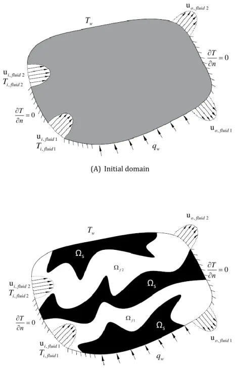
4.5. Heat and mass transfer in bi-fluid topology optimization with fluids separation 126 4.5.1. Initial configuration ... 126

4.5.2. Minimization of fluid power dissipation ... 127

4.5.3. Heat and mass transfer without separation of fluids subdomains ... 127

4.5.1. Heat and mass transfer with separation of fluids subdomains ... 129

4.6. Case study: Double pipe ... 133

4.6.1. Parallel flow ... 133

4.6.2. Counter flow ... 138

4.6.3. Comparison between parallel and counter flows ... 141

4.7. Conclusion ... 144

5. Conclusion and Perspectives ... 147

5.1. Conclusion and limitations ... 147

5.2. Perspectives ... 148 5.2.1. Tridimensional domain ... 148 5.2.2. Turbulent flow ... 149 5.2.3. Numerical methods ... 149 5.2.4. Boundary conditions ... 150 5.2.5. Manufacturing constraints ... 150

vii

List of figures

Figure 1.1: Fluid to fluid heat exchanger ... 8

Figure 1.2:Examples of heat exchangers construction technologies [6] ... 9

Figure 1.3: Common vortex generators used [16] ... 10

Figure 1.4: General algorithm for heat exchanger optimization ... 12

Figure 1.5: Comparison of size, shape and topology optimization ... 13

Figure 1.6:Size, shape and topology optimization applied on heat exchangers ... 14

Figure 1.7: Pareto optimal front in shape optimization[39] ... 19

Figure 1.8: Example of resulting blades from tube tank heat exchanger shape optimization[39]19 Figure 1.9: Topology optimization on mechanical structures problems [47] ... 21

Figure 1.10: Discretized domain in topology optimization. ... 21

Figure 1.11: Topology optimization in heat and mass transfer ... 22

Figure 1.12: Topology optimization results in Stokes flow [66] ... 27

Figure 1.13: Design of a bend pipe using level set method [78] ... 29

Figure 1.14: Design of a diffuser using level set method [78] ... 29

Figure 2.1: Initial guess and final solution of bi-fluid topology optimization problem ... 42

Figure 2.2 Main Loop ... 46

Figure 2.3 Inner Loop ... 47

Figure 2.4 Normal Distribution function for and . ... 48

Figure 2.5 Mono-eta interpolation function for inverse permeability coefficient ... 49

Figure 2.6: Constraint functions for fluid 1 and fluid 2. ... 50

Figure 2.7: Interpolation function (2.10) for different values of ... 51

Figure 2.8:Bi-eta interpolation function ... 53

Figure 2.9 Constraint function for fluid 1 (A) and fluid 2 (B) in a single cell ... 54

Figure 2.10: Representation of a control volume ... 55

Figure 2.11: Distribution of transport quanitites and their coefficients ... 56

Figure 2.12: Initial configuration of double pipe example for mono-eta formulation ... 68

Figure 2.13: Topology optimization results for various initial values of ... 69

Figure 2.14: Mono-eta interpolation function for double pipe configuration ... 70

Figure 2.15: Bi-eta topology optimization of double pipe domain ... 71

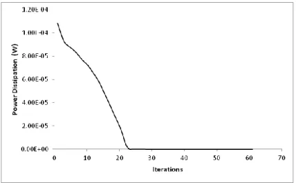
Figure 2.16: Variation of power dissipation objective function throughout the optimization process ... 72

Figure 2.17: Variation of power dissipation objective function from iterations 24 to 60 ... 72

Figure 2.18 Single pipe configuration (A) and its optimisation result (B) ( field) using bi-eta interpolation function for and (B) ... 73

Figure 2.19: Topology optimization result for ... 74

Figure 2.20 Topology optimization of single pipe with ... 75

Figure 2.21: Initial configuration of diffuser case ... 76

Figure 2.22: Calculation of global power dissipation ... 77

Figure 2.23: Calculation of local power dissipation ... 78

viii

Figure 2.25: Initial configuration of bend pipe case ... 79

Figure 2.26 Topology optimization results of bend pipe case ... 80

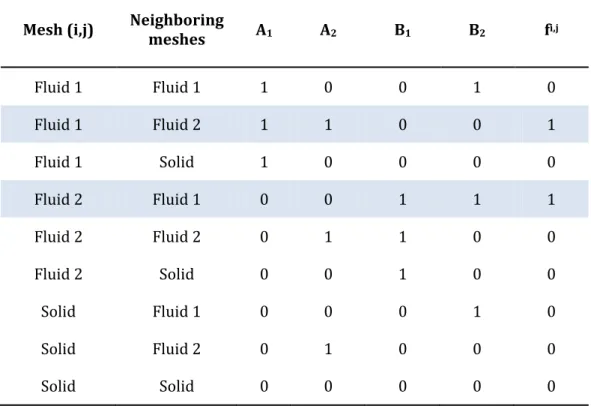
Figure 3.1: (i,j) Mesh and its neighbor meshes ... 88

Figure 3.2: Double pipe example with fluid separation using continuity objective function ... 90

Figure 3.3: Variation of power dissipation objective function throughout the optimization process ... 91

Figure 3.4: Variation of Multi objective function throughout the optimization process ... 92

Figure 3.5: Double diffuser configuration ... 92

Figure 3.6: Results of double diffuser example without continuity objective function ... 93

Figure 3.7: Results of double diffuser example with continuity objective function ... 93

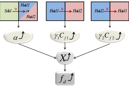
Figure 3.8: Summary of separation of fluids subdomains using the inverse permeability coefficient ... 94

Figure 3.9: Penalization functions, , and ... 96

Figure 3.10: Comparison of fluid dissipation function for different fluid mixtures ... 97

Figure 3.11: Comparison of power dissipation due to fluid friction, with and without fluid separation ... 98

Figure 3.12: Topology optimization result for double diffuser configuration with the modified inverse permeability coefficient ... 99

Figure 3.13: Initial domain configuration ... 100

Figure 3.14: Optimization results for double pipe configuration using constraint function technique for fluid separation ... 101

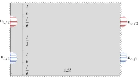
Figure 3.15: Initial configuration of double pipe example with AR=1.5; parallel flow ... 102

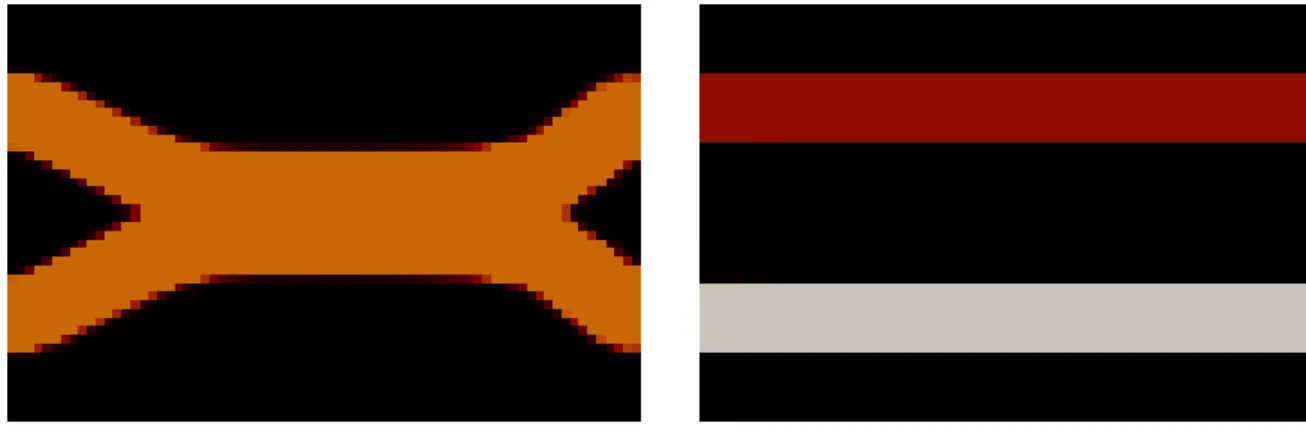
Figure 3.16: Topology optimization results of double pipe example in parallel flow, (A) without fluids phases separation and (B) with fluid phases separation. ... 103

Figure 3.17: Initial configuration of double pipe example with AR=1.5; counter flow ... 104

Figure 3.18: Topology optimization results of double pipe example in counter flow, (A) without fluids phases separation and (B) with fluid phases separation. ... 104

Figure 3.19: Minimization of fluid power dissipation with fluid phases separation, in parallel flow (red curve) and counter flow (blue curve) ... 105

Figure 4.1: Configurations of single pipe case ... 117

Figure 4.2: Topology optimization result for single pipe by minimization of ... 118

Figure 4.3: Temperature and velocity profiles at velocity exit boundary for cases A, B and C for Re=10 ... 119

Figure 4.4: Temperature and velocity profiles at velocity exit boundary for cases A, B and C for Re=500 ... 120

Figure 4.5: Topology optimization result of single pipe by maximization of : case A ... 121

Figure 4.6: Topology optimization result of single pipe by maximization of : case B ... 122

Figure 4.7: Temperature fields of optimal results of cases A and B ... 123

Figure 4.8: Horizontal temperature of the central core for structures A and B ... 123

Figure 4.9: Variation of in function of for structure B ... 124

Figure 4.10: Topology optimization result of single pipe by maximization of : case C ... 124

Figure 4.11: Velocity and temperature fields of case C ... 125

Figure 4.12: Variation of in function of for optimal structures of cases B and C for ... 125

Figure 4.13: Initial configuration of double pipe with fluid inlet and outlet boundaries on the same edge ... 126

ix

Figure 4.14: Topology optimization results: Minimization of fluid power dissipation without

fluid separation (A) and with fluid separation (B) ... 127

Figure 4.15: Topology optimization results of heat and mass transfer without fluid separation for (A) and (B) ... 128

Figure 4.16: Variation of and throughout the optimization process for without fluid separation ... 129

Figure 4.17: Topology optimization result of heat and mass transfer with fluid separation for ... 130

Figure 4.18: Variation of and throughout the optimization process for with fluid separation ... 130

Figure 4.19: Topology optimization result of heat and mass transfer with fluid separation for ... 132

Figure 4.20: Initial configuration of double pipe with parallel flow arrangement ... 133

Figure 4.21: Double pipe configuration with parallel flow arrangement: structure variation with respect to the weighting factor ... 135

Figure 4.22: Geometrical parameters that reflect the trade-off between pressure drop and heat transfer ... 136

Figure 4.23: Fluid power dissipation for various bending angles ... 136

Figure 4.24: Double pipe with parallel flow arrangement: Pareto frontier ... 138

Figure 4.25: Initial configuration of double pipe with counter flow arrangement ... 138

Figure 4.26: Double pipe configuration with counter flow arrangement: structure variation with respect to the weighting factor ... 140

Figure 4.27: Double pipe with parallel flow arrangement: Pareto frontier ... 141

Figure 4.28: Fluid power dissipation and heat transfer objective function variation in function of weighting factor for parallel and counter flows arrangements ... 142

Figure 4.29: Outlet temperatures of cold and hot streams variation in function of weighting factor for parallel and counter flows arrangements ... 142

Figure 4.30: Outlet temperature of cold and hot streams throughout optimization process in parallel and counter flows for ... 143

Figure 4.31: Optimal structures for high values of in parallel flow and counter flow topology optimization ... 143

x

List of tables

Table 1.1: Summary of applications of topology optimization on heat and mass transfer

problems ... 31

Table 2.1: Objective function of topology optimization result of Figure 2.13 ... 68

Table 2.2: Investigation of topology optimization results of the bend pipe case ... 80

Table 3.1: Continuity function coefficients at extremum values of and ... 89

Table 4.1: Properties of fluid 1, fluid 2 and solid ... 117

Table 4.2: Investigation of topology optimization results ... 121

Table 4.3: Thermal and hydraulic performance of topology optimization results for and ... 128

Table 4.4: Thermal and hydraulic performance of topology optimization results for various values of weighting factor ... 131

Table 4.5: Thermal and hydraulic performance of topology optimization results for various values of ... 134

Table 4.6: Geometrical parameters and of for structures of ... 137

Table 4.7: Thermal and hydraulic performance of topology optimization results for various values of weighting factor ... 139

xi

Nomenclature

Heat flow Mass flow rate Temperature

Heat capacity Nusselt number

Heat transfer coefficient Thermal conductivity Interpolation function Penalization parameter Reynolds number Time Normal vector Velocity Pressure Body force

Horizontal component of velocity Vertical component of velocity Multi-objective function G Constraint function Loop index Number of elements Surface Pentadiagonal matrix Source term vector

FVM central coefficient FVM west side coefficient FVM east side coefficient FVM south side coefficient

FVM north side coefficient Weight factor

Residual function Lagrange function

Upper and Lower asymptotes Quantity

Inverse permeability coefficient Convective term

Diffusive term

Greek letters

Friction factor Porosity limit

Generic scalar for interpolated parameters

Design parameter Spatial set

Boundary Density

Inverse permeability coefficient Fluid dynamic velocity

Residual

Transport property Wall shear force Adjoint vector

Absorption term for fluid-fluid separation

Subscripts

xii

Abbreviations

LMTD Logarithmic mean temperature difference

NTU Number of transfer units AM Additive manufacturing SLS Selective laser sintering 3D Three dimensional 2D Bi dimensional

CAD Computer aided design

SIMP Solid Isotropic material with penalization

RAMP Rational approximation of material properties

ESO Evolutionary structural optimization BESO Bi-directional evolutionary

structural optimization FEM Finite element method FVM Finite volume method

MMA Method of moving asymptotes GCMMA Globally convergent method

of moving asymptotes CDS Central differencing scheme

QUICK Quadratic upstream interpolation for convective kinetics

1

Chapitre 1: Introduction Générale

1. Motivation et Objectifs

Un grand nombre d’études et de recherches sont menées pour améliorer la performance des systèmes énergétiques et optimiser leur efficacité, en profitant de l’avancement des algorithmes mathématique d’optimisation et de la capacité de calcul des ordinateurs. Cependant 80% de l'utilisation de l'énergie est impliquée dans le transfert de chaleur. Cela souligne l'importance majeure des échangeurs de chaleur et leur implication dans presque tous les systèmes énergétiques. Ils sont utilisés dans des applications telles que les procédés, la production et la conversion d'énergie, le transport, la climatisation et la réfrigération, la récupération de chaleur et les industries de stockage et de fabrication. Les échangeurs de chaleur sont des dispositifs utilisés pour transférer de la chaleur entre deux fluides ou plus, ou entre un objet solide et un fluide, généralement sans interaction de travail.

Le plus simple échangeur de chaleur est celui à double tuyau, un pour le flux froid et un autre pour le flux chaud séparés par une certaine épaisseur. Ce type d’échangeur est le moins efficace et compact, par conséquent, plusieurs technologies de construction d'échangeurs de chaleur ont été développées au cours des années, parmi lesquelles on peut citer les plus importantes : échangeur à plaques, échangeur tubes ailettes, échangeur tubes calandre, etc.

De nombreuses études et recherches ont été menées pour améliorer le transfert de chaleur dans les échangeurs de chaleur, par l'insertion de dispositifs de perturbation de l'écoulement (ailettes persiennes, générateurs de tourbillons, etc.) et la modification de la rugosité des surfaces de transfert de chaleur. Néanmoins, il existe beaucoup de théories d'idéalisation dans la conception des échangeurs de chaleur pour obtenir une meilleure performance globale. Par exemple, concevoir des échangeurs de chaleur ayant des débits égaux dans tous les canaux [14], ou régler l'équilibre du coefficient de transfert thermique de chaque côté de l'échangeur de chaleur [15]. Cependant, l’amélioration de la performance des échangeurs de chaleur est une procédure plus sophistiquée que de simplement utiliser des techniques pour augmenter le coefficient de transfert de chaleur, ou considérer des théories d'idéalisation. Ceci est dû à de nombreux facteurs intervenant dans l'échangeur de chaleur. Le taux de transfert de chaleur et la perte de charge due au frottement du fluide, sont les phénomènes physiques, toujours en opposition, influençant le plus les caractéristiques de l’échangeur. Ainsi l’optimisation des échangeurs de chaleur a été un domaine d'étude et de recherche intensif, pour sa capacité à améliorer la performance des échangeurs de chaleur et leur efficacité en prenant compte de tous les facteurs en opposition et les limitations de conception.

C’est pourquoi l'amélioration des performances des systèmes, y compris les échangeurs de chaleur, dépend de la capacité à répondre aux spécifications demandées pour l'échangeur de chaleur lui-même. L'objectif de cette recherche est de repousser les limites des connaissances et de développer des outils et des méthodes pour permettre la création d'une nouvelle génération d'échangeurs de chaleur. Le nouveau concept développé est basé sur les méthodes les plus récentes et les plus complexes dans le domaine de l'optimisation de la configuration, les

2

techniques d'optimisation topologiques qui ne sont pas basées sur une géométrie prédéfinie. Ces méthodes permettent d'atteindre une architecture complexe et efficace basée strictement sur les objectifs et contraintes définis. L'état actuel des travaux scientifiques permet l'application de l'optimisation topologique aux échangeurs de chaleur comprenant un seul fluide et un solide. Le présent travail vise à étendre les méthodes d'optimisation topologique en mécanique des fluides à des cas incluant deux fluides, ce qui est le cas pour les échangeurs de chaleur fluide-fluide. Cependant, une attention devrait être accordée à la complexité des géométries générées par l'optimisation de la topologie. Une grande question se pose donc: comment ces structures seront-elles fabriquées en particulier pour la production à grande échelle? L'avancement dans la technologie de fabrication additive est la réponse évidente à cette question. Il est donc très utile d'associer l'impression 3D à l'optimisation topologique, pour le développement d'une nouvelle méthode innovante dans la conception et l'optimisation des échangeurs de chaleur.

2. Optimisation des échangeurs de chaleur

L'optimisation est le mécanisme de sélection de la meilleure solution dans une situation particulière soumise à un certain nombre d'obstacles et de limitations. Le critère qui définit la meilleure solution est la fonction objectif. Les limitations sur les solutions disponibles sont définies par les contraintes. Ce qui décrit différentes solutions sont les variables de problème auxquelles nous essayons d'assigner les meilleures valeurs pour minimiser ou maximiser la fonction objectif. La façon dont nous pouvons réaliser le processus d'optimisation est définie par l'algorithme d'optimisation que nous utilisons. Si l'on veut optimiser une fonction objectif f (x) = x, la meilleure solution est simplement infinie. Ainsi, un problème d'optimisation n'a aucun sens s'il n'y a pas de conflit entre plusieurs fonctions objectifs ou entre une fonction objectif et une contrainte. De même, dans les échangeurs de chaleur, s'il n'y a pas de limitation sur le volume ou la masse ou si l'on ne tient pas compte de la perte de charge, l'échangeur de chaleur optimal pour avoir un transfert de chaleur maximal est celui ayant une longueur infinie. Les variables du problème d’optimisation des échangeurs de chaleur peuvent être les conditions de fonctionnement de l’échangeur, propriétés physiques des matériaux et les fluides et les paramètres géométriques du dispositif.

Les problèmes d'optimisation, dans lesquels les paramètres géométriques sont les paramètres d'optimisation, sont classés en trois catégories selon le degré de liberté et la possibilité de modifier la géométrie: optimisation de taille, de forme et topologique. Dans l'optimisation de la taille, les variables du problème mathématique sont les paramètres géométriques de la structure telle que la longueur, la largeur, le rayon, etc. La forme et la connectivité des éléments entre elles sont connues et fixées. Par conséquent, la solution optimale finale est très similaire à la conception de base initiale. L'optimisation de forme augmente le degré de liberté du problème, où elle peut changer la taille et la forme simultanément en ajoutant des variables capables de déformer la forme de la structure (par exemple modifier la forme des canaux d’écoulement). Cependant, l'architecture de la structure est toujours similaire à la conception initiale, puisque la topologie globale de l'échangeur de chaleur ne peut pas être modifiée. Enfin, en optimisation topologique, chaque maille du domaine d'optimisation est un paramètre de conception; ce qui permet d'ajouter ou de supprimer du matériel dans chaque point de l'espace de conception sans être limité à une topologie initiale. Cela augmente considérablement le nombre de variables dans le problème d'optimisation, ce qui

3

rend la convergence plus difficile. Cependant, l'optimisation topologique est devenue si attrayante pour sa capacité à atteindre des configurations innovantes et complexes basées strictement sur les objectifs et contraintes définis. L'optimisation de la taille et de la forme a été largement appliquée à l'optimisation des échangeurs de chaleur, tandis que l'optimisation topologique est encore limitée aux échangeurs de chaleur fluide-solide.

Les deux critères principaux les plus utilisés dans les problèmes d’optimisation des échangeurs de chaleur sont les suivants : les critères basés sur les irréversibilités thermodynamiques, comme la minimisation de la génération d’entropie et/ou de la dissipation de l’entrasse, et les critères économiques qui consistent à minimiser le coût du fonctionnement et le coût initial de l’échangeur. Il existe de nombreux autres critères d'optimisation, comme la diminution de la perte de charge totale, augmentation du taux de transfert thermique, diminution de la température maximale ou moyenne, ou par exemple minimisation de la masse totale de l'échangeur de chaleur dans l'industrie aéronautique, etc.

3. Optimisation topologique

L'optimisation topologique a été développée à l'origine pour l'optimisation des problèmes de structures mécaniques. L'objectif était de trouver la forme qui utilise le minimum de matière tout en maintenant les contraintes mécaniques inférieures à un niveau acceptable. L'optimisation topologique a été définie par Bendsoe et Sigmund [45] comme une optimisation de forme des structures qu'elle devrait définir à chaque point de l'espace de conception s'il existe un matériau ou non, la topologie de la structure n'étant pas fixée a priori. Ainsi, à partir d'un domaine initial vide, complet ou dans n'importe quel état intermédiaire, les paramètres de contrôle utilisés permettent de créer sans restriction des créations de trous et d'agglomérats de matériaux, afin de trouver la meilleure topologie possible. Récemment, le concept d'optimisation topologique a été appliqué à un large éventail de disciplines physiques comme les mécaniques des fluides, le transfert de chaleur, l'acoustique, l'électromagnétique et l'optique. Dans les problèmes de transport de masse et chaleur en optimisation topologique, l’objectif était de trouver l’architecture optimale qui correspond à un compromis entre la minimisation de la perte de charge et la maximisation de transfert de chaleur. Cependant, la mise en œuvre de méthodes d'optimisation topologique est assez complexe car elle nécessite un algorithme capable d'allouer et de réallouer efficacement le matériel dans un domaine ayant les dimensions et les conditions aux limites prédéfinies.

En optimisation topologique, l'espace de domaine est discrétisé en des petites mailles, également appelés cellules, où chaque cellule contient une variable de conception adimensionelle. Les valeurs de toutes les variables de conception dans toutes les cellules définissent la forme de la structure entière. Ainsi, le problème d'optimisation est de trouver les valeurs optimales de toutes les variables de conception, en minimisant une certaine fonction objectif en respectant les fonctions contraintes, qui sont généralement des fonctions de porosités qui limitent le volume maximal de l’une des matières dans le domaine d’optimisation.

Il existe deux grandes familles de méthodes de la résolution du problème d'optimisation topologique: les approches discrètes et les approches continues, qui correspondent

4

respectivement aux méthodes dans lesquelles le paramètre local contrôlant le matériau dans chaque cellule peut prendre des valeurs discrètes, ou des valeurs bornées continues. Ces méthodes dépendent du gradient des fonctions objectifs et des contraintes. Le grand nombre de variables de conception et la nécessité de calculer la dérivée totale de la fonction objectif par rapport aux variables nécessitent des techniques mathématique avancées pour assurer la convergence du vecteur de variables vers la solution optimale. L'optimisation topologique est devenue un domaine de recherche bien développé avec de nombreuses techniques pour traiter les problèmes d'instabilité numérique fréquemment rencontrés dans l'optimisation topologique tels que les damiers, les dépendances de maillage et les minima locaux.

4. Méthodes d’optimisation topologiques

Les méthodes d'optimisation topologiques visent à forcer le paramètre de conception à prendre progressivement des valeurs discrètes, éliminant ainsi les régions grises et conduisant à un domaine noir et blanc, où les variables de conception dans chaque cellule sont égales à 0 ou 1 (solution 0-1). Cependant, il existe aussi des méthodes qui peuvent résoudre des problèmes combinatoires discrets et qui sont appelés approches discrètes. Nous allons considérer un problème d'optimisation topologique où nous cherchons la distribution optimale des deux phases A et B. Dans les approches discrètes, la phase à l'intérieur de la cellule est modifiée en une seule étape entre A et B (hard-kill). Dans les approches continues, une petite quantité de phase A est remplacée par la phase B ou vice-versa dans chaque étape, jusqu'à ce que nous atteignions à la fin du processus d'optimisation une cellule complètement correspondante à A ou B (soft-kill).

Les méthodes d'optimisation topologique reposent sur trois parties principales: le solveur direct du problème physique (éléments finis, volumes finis, ...), la méthode d'analyse de sensibilité (adjoint discret, adjoint continu, ...) pour calculer la dérivée totale des fonctions objectifs et contraintes par rapport aux variables de conception, et un optimiseur numérique.

La méthode la plus rencontrée en optimisation topologique en transfert de masse et chaleur est la méthode de densité. Cette méthode consiste à utiliser une fonction d'interpolation pénalisée pour calculer les quantités physiques dans chaque cellule, par ex. la rigidité du matériau dans les problèmes de structure mécanique et la conductivité thermique dans les problèmes de conduction de chaleur etc., en fonction des variables de conception continue. Le principal défi des méthodes de densité est l'introduction d'une fonction d'interpolation capable d'orienter la solution vers des valeurs 0-1 discrètes et d'omettre des valeurs intermédiaires de la variable de conception, tout en assurant une représentation physique réelle des matériaux fictifs correspondant à des densités intermédiaires, connus sous le nom de matériaux gris, qui doivent être entièrement éliminés quand le problème converge vers la solution finale. Un schéma d'interpolation populaire pour satisfaire les conditions ci-dessus est la formule SIMP (Solid Isotropic Material with penalization).

Les méthodes de level set sont des techniques computationnelles introduites en 1988 par Osher et Sethian [58] pour le suivi des interfaces mobiles. L'idée principale des méthodes level

5

set est d'introduire une fonction dépendant du temps et de l'espace qui définit l'interface entre les deux matériaux présents dans le problème d'optimisation.

L’approche évolutive ESO (Evolutionary structural optimization) qui utilise des variables de conception discrètes, a été introduite par Xie et Steven [61] pour l'optimisation des structures mécaniques. Cette méthode est basée sur le concept simple de retrait progressif d’un matériau inefficace d'une structure jusqu'à ce que la contrainte déterminant le volume de matériau dans le domaine de conception soit satisfaite. Yang et al. a développé l'Optimisation structurelle évolutive bidirectionnelle (BESO), une version améliorée de l'ESO, qui permet de retirer et d'ajouter le matériau simultanément [62]. Le retrait et l'addition de matière sont basés sur la valeur du nombre de sensibilité. Les approches évolutives (ESP et BESO) ont été largement appliquées aux problèmes de structures mécaniques avec de nombreuses techniques développées pour faire face aux difficultés rencontrées en raison de l'aspect discret du problème. Dans la conduction de chaleur pure, les approches évolutives étaient également applicables mais les résultats ont montré que la méthode conduit à l'optimum local. Par conséquent, les approches évolutives ne se sont pas intéressantes pour l'optimisation de la topologie de la mécanique des fluides.

5. Conclusion

L'optimisation topologique dans les problèmes d'écoulement était initialement limitée à de faibles nombres de Reynolds et à un état stationnaire (écoulement de Stokes) sans tenir compte des effets d'inertie. Ensuite, divers auteurs ont étendu la procédure d'optimisation pour couvrir une plus large gamme de nombre de Reynolds, des effets d'inertie (flux de Darcy-Stokes et de Navier-Stokes), des forces corporelles non uniformes et des flux instationnaires.

Malgré l’attention portée aux techniques évolutives dans les problèmes de structure mécanique et problèmes de transfert de chaleur par conduction, elles n'ont pas été prises en compte dans les problèmes d'écoulement des fluides selon la revue de la littérature. La méthode Level Set a été trouvée attrayante pour les problèmes d'écoulement en raison de leurs résultats dans des simulations numériques 2D et 3D pour divers types de flux. Cependant, cette méthode peut seulement évoluer à partir des interfaces existantes et n’est pas capable de générer de nouveaux trous, ce qui signifie qu'il est impossible de générer de nouveaux canaux dans l'optimisation des écoulements. Ceci est considéré comme un inconvénient conceptuel de la méthode, surtout si elle sera utilisée pour l'optimisation topologique des échangeurs de chaleur. La nucléation de nouveaux trous dans Level Set a été possible en la combinant avec la méthode Topological Sensitivity. Cette méthode combinée a été appliquée et testée par divers auteurs. Les résultats montrent que la solution finale reste fortement dépendante de l'estimation initiale.

La méthode de densité est complètement indépendante de l’estimation initiale et la génération de canaux et de structures complexes dépend uniquement des fonctions d'objectifs et des contraintes. De plus, la revue littérature a montré que la méthode de densité a été appliquée sur la majorité des problèmes liés au transfert de chaleur et de masse. Malgré la nécessité d'un temps de calcul élevé, la méthode de densité semble être la méthode la plus appropriée pour

6

étendre l'application de l'optimisation topologique en mécanique des fluides au domaine bi-fluide, ce qui n'était pas envisagé auparavant.

6. Plan de la thèse

L'algorithme général de la méthode de densité est composé de trois étapes principales :

 Le solveur CFD utilisant la méthode des volumes finis.

 L'analyse de sensibilité basée sur la méthode d’adjoint discret.

 La méthode des asymptotes mobiles comme optimiseur numérique.

Le reste du document est divisé comme suit:

 L'algorithme détaillé de la méthode d'optimisation présenté ci-dessus et le développement détaillé de chaque partie de la méthode sont présentés au chapitre 2. Deux formulations différentes seront comparées, l'une utilisant une variable de conception unique dans chaque cellule de conception et la seconde utilisant deux variables de conception. Dans chaque cellule de conception qui double le nombre de variables du problème.

 La séparation des fluides sera examinée au chapitre 3, où chaque fluide doit prendre son propre trajet dans le domaine d’optimisation indépendamment de l’autre.

 Dans le chapitre 4, la maximisation du transfert de chaleur entre les deux fluides séparés sera considérée.

7

Chapter

1

1.

General

Introduction

1.1. Introduction

1.1.1. Motivation

In the 2015 United Nations climate change conference held in Paris, representatives of 196 nations adopted a long term strategy to respond to the threats of climate change and deal with greenhouse gas emissions mitigation plans. The agreement, known as “Paris agreement”, aimed to limit the rise in global average temperature by holding it this century below 2°C above pre-industrials level [1]. As part of this agreement, the French environment minister announced in July 2017 his country plan to attain neutral carbon equilibrium in 2050, by reducing human carbon emissions to the level of ecosystems carbon’s absorption capacity [2]. The French plan also considered a four billion Euros investment to increase energy efficiency and stop coal usage for electricity production by 2022 [3]. Beside the problems related to global warming and climate change, energy management policies face various challenges. First, population growth increases the demand for energy services [4]. Furthermore, the increase in the ratio of urban population to rural population augments the demand on energy even more. Second, an increase in gross domestic product (GDP) is associated with an increase in energy consumption, which tend to vary according to the GDP growth in different economy sectors [5]. Energy market is also influenced by many other sectors, as technology innovations, oil and gas prices, carbon emissions pricing by some governments, etc. All these reasons explain the studies and researches conducted to improve the performance of energy systems and optimize their efficiency, by taking advantage of advancements in mathematical optimization tools and computers calculation capacities.

8

On the other hand, about 80% of energy utilization is involved in heat transfer. This highlights the major importance of heat exchangers and their involvement in nearly every energy system. They are used in applications such as processes, energy production and conversion, transport, air conditioning and refrigeration, heat recuperation and storage and manufacturing industries. Heat exchangers are devices used to transfer heat between two or more fluids, or between a solid object and a fluid usually without work interactions. Usually, fluids do not mix in heat exchangers, and heat is transferred through a dividing wall without fluid leakage. However, there are still some types of heat exchangers where fluids enter in direct contact and are later separated. In this case, heat transfer is mainly caused by phase change enthalpy[6]. Figure 1.1 shows a general representation of a fluid to fluid heat exchanger. and stand respectively for temperature, pressure and thermal heat transfer load. Subscripts and stands respectively for inlet, outlet, cold and hot. The heat exchanger is characterized by the total heat thermal power transferred from the hot stream to the cold stream, the pressure drop of both fluids: + , and other geometrical parameters like its mass, volume and compactness.

Figure 1.1: Fluid to fluid heat exchanger

The simplest heat exchanger is a double pipe exchanger, with one pipe for cold stream and another one for hot stream. This type of heat exchangers has the lowest efficiency and compactness, hence, a wide range of heat exchangers construction technologies have been developed over the years. Among these technologies, the following are the most known and used (Figure 1.2): tubular heat exchangers, as shell and tubes used for high pressure and temperature flow conditions [6], plate type heat exchangers characterized by a high transfer coefficient but cannot endure high pressure and temperatures flows neither high temperature gradient. There exist many other technologies as extended surface heat exchangers that use fins to increase heat transfer surface, regenerators and adiabatic wheels where heat transfer process is not continuous, etc. Heat exchangers are also characterized by their flow arrangement. We can distinguish three different types: parallel flow where the fluids flow parallel to each other in the same direction, counter flow where fluids flow parallel but in opposite direction and cross flow where fluids flow in perpendicular direction.

Q

T

P

T

P

T

P

T

P

9

(A) Shell and tube heat exchanger (Tubular type) _{(B) Welded plate heat exchanger (Plate type)}

(C) Fin tubes heat exchanger (Extended surface

type) (D) Rotary regenerator (Storage type)

Figure 1.2:Examples of heat exchangers construction technologies [6]

Heat exchanger design is a complex iterative procedure, due to many physical phenomena occurring inside the device, and due to the interactions between these phenomena and their mutual dependency. Thermal design of heat exchangers aims to determine the required heat transfer surface for a fixed heat load duty, or determine the rate of heat transfer for a fixed heat transfer surface. The most used basic thermal design methods are logarithmic mean temperature difference method (LMTD) and effectiveness-number of transfer units’ method (ε-NTU). Mechanical design has also a major importance in heat exchangers design. It aims to handle thermal and pressure stresses, and ensure durability of the device at different operational phases [6].

Many studies and researches were conducted to enhance heat transfer in heat exchangers, by insertion of flow disturbance devices and modification of the roughness of heat transfer surfaces. These techniques enhance heat transfer by making the flow turbulent near heat transfer surface, by breaking the laminar layer of the flow to reduce the thermal resistance and by increasing the residence time of heat transfer fluids. Among these devices we mention: vortex generators [7] (Figure 1.3), louvered fins [8] twisted tapes [9], ribs [10][11], spiral fins[12], circular fins[13], etc. Nevertheless, there exist a lot of idealization theories in heat exchangers design to get a better overall performance. For example designing heat exchangers with equal flow rates in all channels [14], or setting equilibrium in heat transfer coefficient at each side of the heat exchanger [15], etc.

10

Figure 1.3: Common vortex generators used [16]

Enhancing the performance of heat exchangers is quite a more sophisticated procedure than simply using techniques for increasing heat transfer coefficient, or considering idealization theories. This is caused by many trade-off factors occurring inside the heat exchanger. The most important one is the trade-off between heat transfer rate and pressure drop due to fluid friction. If the designer wants to increase heat transfer rate, he could simply decrease the diameter of the tubes but the pressure drop will then increase. In this case, what determines the enhancement of the heat exchanger’s performance is the cost of the pumping power due to the pressure drop versus the benefit of the recovered thermal power. Another example is the trade-off between the capital cost and the operating cost where a more efficient heat exchanger may decreases the operating cost but requires a higher capital cost and vice versa. Design of heat exchangers is also subject to many constraints, which vary according to the application, like total weight and volume, design limitations to avoid corrosion, fatigue failure, etc. Optimization of heat exchangers consists of finding a compromise between all trade-off factors within the feasible solutions that respect all design constraints, by minimizing a certain objective or optimization criteria.

Heat exchangers optimization has been an intensive field of study and research, for its capability to improve the performance of heat exchangers and their efficiency while taking into account all trade off factors and design limitations. Dimitrios et al. [17] conducted an optimization of heat exchangers mounted on the hot gas exhaust nozzle of an intercooled recuperated aero engine. The optimization resulted in two new recuperators, which were compared with the initial baseline design on the basis of their weight and specific fuel consumption of the aero engine. The initial non-optimized heat recuperator was capable of achieving 12.3% reduction in fuel consumption in relation to a non intercooled aero engine. The first optimized recuperator increased fuel consumption reduction to 13.1% in relation to non intercooled aero engine, while reducing the weight of the recuperator by 5%. The second optimized recuperator was less efficient regarding fuel consumption, whose reduction in relation to a non intercooled engine dropped to 9.1%, but on the other hand the total weight was reduced by 50% in relation to the initial non optimized recuperator.

Ghadamian et al [18] optimized the operation conditions of heat exchanger used for heat recuperation in a cement industry. They were able to increase heat recuperation by 592.2 Kw/year without any increase in cost. Heat exchanger used for waste heat recovery in industry

11

was also considered by Yildirim and Soylemez [19]. Their resulted optimized plate heat exchanger achieved approximately 0.91 million $ net profit over 10 years life cycle, whereas the initial heat exchanger was only capable of saving around 0.78 millions.

Caputo et al. [20] tested the effectiveness of an optimization method on several heat exchangers installed in chemical plants. A shell and tube Soda-water heat exchanger weight was reduced from 5.287 Kg to 2.697 Kg, whereas pressure drop was decreased from 5.5 kPa to 1.7 kPa on shell side and remained approximately the same on tube side. Another potassium hydroxide-water heat exchanger was studied, where a 58% reduction in weight was achieved. The pressure drop in the optimized heat exchanger was increased from 5 to 8 kPa on the shell side, but on the tube side the pressure drop was significantly reduced from 48.4 kPa to 7 kPa. All this improvement resulted in a better performance regarding operational cost, and the heat exchanger became shorter and more compact.

Gholap and Khan [21] provided a multi-objective optimization of a heat exchanger used in refrigeration where they showed the trade-off between energy consumption and material cost. Regarding energy consumption, the best design presented a reduction of 8.92 % in relation to the baseline design, but it needed a 50.19 % increase in material cost. The best achievement in term of material cost was a reduction by 41.82% at the expense of a 6.15% increase in energy consumption on a daily basis. In that case, heat exchangers optimization provides best trade-off solutions, and the choice of a final design is based on the designer strategy regarding the competing objectives. This brief literature review shows the advantage and profit gained by using advanced optimization tools in heat exchangers design.

1.1.2. Research objectives

As seen in the last paragraph, improving the performances of systems including heat exchangers depends on the ability to meet the specifications requested for the heat exchanger itself. The objective of this research is to push the limits of the knowledge base and develop tools and methods to enable the creation of a new generation of heat exchangers. The new design concept developed is based on most recent and complex methods in the field of configuration optimization, the topology optimization techniques which are not based on predefined geometry. These methods allow reaching a complex and efficient design based strictly on the defined objectives and constraints. The current state of scientific work allows the application of topology optimization to heat exchangers including a single fluid and a solid. The present work aims to extend the topology optimization methods in fluid mechanics to cases including two fluids, which is the case for fluid-fluid heat exchangers. Meanwhile, an attention should be given to the complexity of geometries generated by topology optimization. Hence, a big question arises: how these structures will be manufactured especially when it comes to large scale production? The advancement in additive manufacturing technology is the obvious answer to this question. Additive manufacturing is the process of adding layer upon layer of a given material. It reads information from a computer-aided design (CAD) file to add successive layers of materials to fabricate the designed object. The first use of additive manufacturing was limited to create prototype or visualize a part for presentations purposes. However, currently the additive manufacturing is used to produce end-use products for a wide range of applications

12

such as aircraft parts, automobile, medical equipments etc. Therefore, the advance in 3D printers technologies raised interest in topology optimization development and application in various engineering industries. It is then very useful to associate 3D printing with topology optimization, for the development of a new generation in heat exchangers design and optimization.

1.2. Heat exchangers optimization

1.2.1. Introduction to optimization problem

Figure 1.4: General algorithm for heat exchanger optimization

Optimization is the mechanism of selecting the best solution in a particular situation subject to a number of obstacles and limitations. The criterion that defines the best solution is the objective function. The limitations on available solutions are defined by the constraints. What describe different solutions are the problem variables to which we are trying to assign the best values to minimize or maximize the objective function. How we can achieve the optimization process is defined by the optimization algorithm we’re using. If one wants to optimize an objective function , the best solution is simply infinite. Hence, an optimization problem has no sense if there is not a conflict between many objective functions or between an objective function and a constraint. Similarly, in heat exchangers, if there is no limitation on volume and mass or there is no consideration to pressure drop, the optimal heat exchanger regarding heat transfer is the one having an infinite length. Figure 1.4 represents a general schematic for heat exchangers optimization. In next paragraphs most encountered optimization variables, criteria and numerical algorithms in heat exchangers optimization are presented.

Initial variables X0

Objective function evaluation (CFD, correlations …) Optimal criterion met? Optimization algorithm change X END YES NO

13

1.2.2. Optimization variables

The design variables in heat exchangers optimization problems are classified as follows:

 Operating conditions of the heat exchanger (mass flow rate of hot or cold stream, terminal temperatures, etc…)

 Material properties (thermal conductivity, surface roughness, etc….)

 Geometrical parameters that defines the optimal architecture of the heat exchanger.

Figure 1.5: Comparison of size, shape and topology optimization

Optimization problems, in which the geometrical parameters are the optimization parameters, are classified under three categories according to the degree of freedom, and the capability of changing the geometry: size, shape and topology optimization, represented in Figure 1.6. In size optimization the problem variables are the geometrical parameters of the structure such as length, width, radius etc. The shape and the connectivity of the elements between them are known and fixed. Hence, the final optimal solution is very similar to the initial baseline design.

Shape optimization increases the degree of freedom of the problem, where it can change the size and the shape simultaneously by adding variables able to deform the boundaries of the structure. However, the architecture of the structure is still similar to the initial design, since the global topology of the heat exchanger cannot be varied. Finally, in topology optimization, every mesh in the optimization domain is a design parameter; which allows adding or removing material in every point in the design space without being limited to an initial topology. This increases significantly the number of variables in the optimization problem what make it more difficult to converge, as seen in Figure 1.5. However, topology optimization has become so appealing for its capacity to reach innovative and complex configurations based strictly on the defined objectives and constraints. Size and shape optimization have been widely applied on optimization of heat exchangers, whereas topology optimization is still limited to fluid to solid heat exchangers.

Size Shape Topology

Design freedom & Complexity

Optimization difficulty & Result’s performance

14

(A) Size optimization: Initial design _{(B) Size optimization: Final design}

(C) Shape optimization: Initial design (D) Shape optimization: Final design

(E) Topology optimization: Initial design (F) Topology optimization: Final design Figure 1.6: Size, shape and topology optimization applied on heat exchangers

15

1.2.3. Numerical optimization algorithms

Optimization techniques were subject to a considerable progress since early fifties of the twelve century, with the advancement in digital computers and electronic calculation capacities. Optimization algorithms vary according to the information and the method used to search for the next better solution. There exist in literature a wide variety of available optimization algorithms, classified under many criteria, as their capability to reach local of global optimum, their dependency or no on gradient information, the use of single trajectory or a population, etc. In the following, the most used optimization algorithms in engineering problems will be presented and classified as gradient-based and gradient-free algorithms.

 Gradient-based algorithms: this family of optimization algorithm uses the derivative of the objective function as a direction to reach the optimum. The major advantage of these methods is that they can solve optimization problems with an extremely large number of variables. However, their major drawbacks are that they can locate a local optimum and that they are complex to implement. The essential part in calculation time in these algorithms is dedicated to the evaluation of the sensitivity of the objective function. Among most popular gradient based algorithms used, Fletcher-Reeves for unconstrained problem and the Sequential Linear Programming (SLP) and Sequential Quadratic Programming (SQP) [22] for constrained optimization problems..

 Gradient-free algorithms: the most popular family of this type of optimization techniques are the evolutionary algorithms, which are based on phenomena from nature to evolve toward optimal solution. Evolutionary algorithms are easy to implement, and can reach usually global or near global optimal solution. On the other side, evolutionary algorithms suffer from not being able to handle high number of variables and are computational costly. Genetic algorithm [23] is the most efficient and popular type of evolutionary algorithms. It is inspired from science of genetics for the survival of the fittest, more specifically Darwin’s theory and Mendel’s law for genetic evolution and inheritance. It uses biological operators such as crossover, mutation and selection. Design points having the best performance regarding the objective function, are used for the next generation of the optimization. Other popular evolutionary algorithms frequently used are the Particle Swarm Optimization and simulated annealing.

1.2.4. Optimization criterions

In this paragraph, the objective functions usually encountered in the optimization of heat exchangers are presented. The two main criterions are thermodynamic and economic aspects, which could also be coupled in the same problem as it will be seen later. There exist many other optimization criterions depending on the application of the heat exchanger, like decreasing the total pressure drop, increasing the heat transfer rate, decreasing the maximum temperature or average temperature, or for example the minimization of total heat exchanger weight in aeronautical industry, etc.

16 1.2.4.1. Thermodynamic criteria

We will start by presenting the thermodynamic irreversibility occurring in a heat exchanger. In heat exchangers, there are two types of losses: losses associated to irreversibility due to heat transfer between two fluids having a certain temperature difference, and losses associated to mass transfer due to friction between fluids and internal walls of the heat exchanger. Regarding fluid flow, the mechanical energy is not conserved, and a part of it is transformed into thermal energy. This part of energy lost during fluid transport process is considered as a measure for irreversibility. Usually, in most physical phenomena, the quantity of energy turned into heat is considered as the quantity of irreversibilities. When it comes to heat transfer itself, thermodynamic quantities as entropy production and exergy destruction are considered as irreversibilities. Heat exchangers optimization using thermodynamic criteria are based on the minimization of these quantity of irreversibilities, more specifically entropy generation and entransy dissipation.

Entropy production was developed by Bejan [24] who defined it as “the thermodynamics

imperfection to heat transfer, mass transfer and fluid flow irreversibilities”. Entropy production

parameter takes into account both transport processes, heat transfer and mass transfer. Hence, in any variation in the heat exchanger’s geometry to increase heat transfer, associated mechanical energy dissipation is simultaneously evaluated and taken into consideration. It should be noted that the distribution of entropy production itself inside the exchange influences the overall exchanger effectiveness. In fact, the minimal total entropy production of the entire system corresponds to the one having the most uniformly possible local entropy production distribution [25].

Entransy dissipation is another physical quantity developed in 2007 by Guo et al. [26] to measure the irreversibilities in a heat transfer process. It is developed to measure the ability of an object (fluid in case of a heat exchanger application) to transfer heat in analogy with the electric capacitance of a body, which describes its charge transfer ability. Xu et al. [27] applied the entransy dissipation theory of Guo. et al. on internal and external fluid flow. Hence, entransy dissipation was able to take into account irreversibilites due to heat and mass transfer simultaneously.

Before the introduction of entransy dissipation, entropy generation number was considered as the main criterion in heat exchanger optimization based on thermodynamic irreversibilities minimization. The recent studies have shown a preference of methods based on entransy dissipation over entropy generation methods. Twenty different heat exchangers were analyzed by Qian et Li [28]. The results showed that the minimum entransy rate corresponds in all the heat exchangers tested to the highest heat transfer rate. The minimum entropy generation suffered for many cases from the entropy generation paradox, where the efficiency of the heat exchangers can be at its maximum, minimum or anything between when entropy generation reaches its minimum [29]. However, it was demonstrated that the two physical quantities are needed to evaluate irreversibility in heat transfer [30]. When the purpose of heat transfer is for heat-work conversion, the entropy generation is a better irreversibility measurement, whereas the entransy dissipation is better when the heat transfer is for heating and cooling purposes [30] [31].

17 1.2.4.2. Economic criterion

The economic criterion consists of minimizing the total cost of a heat exchanger which is the sum of the capital cost and the operating cost. Economic objective is a widely used criterion in optimization of heat exchangers as it reflects directly the purpose of using heat exchangers in the majority of energy systems. In some applications, it is necessary to take into consideration the economic benefit from each degree of temperature recovered by the heat exchanger, versus the price of each kW needed to operate the exchanger. This is not possible in the methods based on the minimization of irreversibility rate alone. The cost function could be used alone as single objective function [32] or used in multi-objective design optimization to find a trade-off between the exchanger cost and its effectiveness [33].

1.2.5. Literature review on fluid-to-fluid heat exchangers optimization

Size optimization

Huang et al. [34] optimized a vertical ground heat exchanger used in HVAC systems, by minimizing entropy generation number using a genetic algorithm. The variables are a set of geometrical parameters and the material conductivity. The entropy generation expression is coupled with the irreversibility caused by fluid friction and heat transfer as a single objective function. His optimal design has an entropy generation number of 12.2% less than the initial design. He analyzed the advantage made by the optimization method from an economical point of view over a 10 years operation period. The results showed that the capital cost is 1.67 % higher for the optimal design, but the operation cost was 7.2% lower. Thus, he achieved a 5.5% net profit in total cost over the operation period. Guo et Xu [35] applied theory of entransy dissipation on size optimization of a shell and tube heat exchanger using a genetic algorithm. He also showed the benefit of splitting entransy dissipation due to heat transfer and fluid flow as two objective functions and used them in a multi-objective optimization instead of a single objective optimization. The advantage of a multi-objective function is that the designer can control the preferences of maximization of heat transfer and minimization of pressure drop. Results showed that in the design of a heat exchanger with fixed heat load, the single objective optimization improves the performance of the heat exchanger. However, when the heat transfer area is fixed, the improvement of the heat exchanger effectiveness is at the expense of increasing the pumping power. The multi objective optimization design can achieve the same effectiveness as single objective design with less consumption in pumping power, in case of fixed heat transfer area.

Huang [36] compared two different optimization methods: a single objective optimization in which entropy generation is the optimization criterion, and a multi objective method where the entropy generation and the total heat exchanger cost are the objective functions. Optimization procedures were applied on a vertical ground heat exchanger to find the optimal values of various geometrical parameters using a genetic algorithm. The heat exchanger optimized by a single objective method has an operating cost 0.8 % lower than a heat exchanger optimized by the multi-objective method, and a 0.82% lower entropy generation number. On the other side, the capital cost is 10% lower for the heat exchanger optimized by the multi-objective method.