HAL Id: hal-02152378
https://hal.archives-ouvertes.fr/hal-02152378
Submitted on 14 Jun 2019
HAL is a multi-disciplinary open access
archive for the deposit and dissemination of
sci-entific research documents, whether they are
pub-lished or not. The documents may come from
teaching and research institutions in France or
abroad, or from public or private research centers.
L’archive ouverte pluridisciplinaire HAL, est
destinée au dépôt et à la diffusion de documents
scientifiques de niveau recherche, publiés ou non,
émanant des établissements d’enseignement et de
recherche français ou étrangers, des laboratoires
publics ou privés.
Optimal placement and sizing of heat pumps and heat
only boilers in a coupled electricity and heating networks
Getnet Tadesse Ayele, Mohamed Tahar Mabrouk, Pierrick Haurant, Björn
Laumert, Bruno Lacarrière
To cite this version:
Getnet Tadesse Ayele, Mohamed Tahar Mabrouk, Pierrick Haurant, Björn Laumert, Bruno Lacarrière.
Optimal placement and sizing of heat pumps and heat only boilers in a coupled electricity and heating
networks. Energy, Elsevier, 2019, 182, pp.122-134. �10.1016/j.energy.2019.06.018�. �hal-02152378�
Optimal placement and sizing of heat pumps and heat only boilers in a coupled electricity
and heating networks
Getnet Tadesse Ayelea,b, Mohamed Tahar Mabroukc, Pierrick Haurantd, Björn Laumerte and Bruno Lacarrièref
a,c,d,f IMT Atlantique, GEPEA, UMR CNRS 6144, F-44307 Nantes, France.
b,e Department of Energy Technology, KTH Royal Institute of Technology, 100 44 Stockholm, Sweden. bgtayele@kth.se (CA)
Abstract
Multi-energy systems are reported to have a better environmental and economic performance relative to the conventional, single-carrier, energy systems. Electrification of district heating networks using heat pumps, and combined heat and power technologies is one such example. Due to lack of suitable modelling tools, however, the sizing and optimal placement of heat pumps is always done only from the heating network point of view which sometimes compromises the electricity network. This paper proposes an integrated optimization algorithm to overcome such limitation. A load flow model based on an extended energy hub approach is combined with a nested particle swarm optimization algorithm. A waste to energy combined heat and power plant, heat pumps (HPs), heat only boiler (HOB), solar photo-voltaic, wind turbines and imports from the neighborhood grids are considered in the case studies. The results show that optimal placement and sizing of HPs and a HOB using the proposed methodology avoids an unacceptable voltage profiles and overloading of the electricity distribution network, which could arise while optimizing only from the heating network point of view. It also shows that up to 41.2% of the electric loss and 5% of the overall operating cost could be saved.
Keywords:
An extended energy hub; Coupled electricity and heating networks; Heat pump; Multi-carrier energy networks; Multi energy systems; Particle swarm optimization (PSO).
1. Introduction
Multi-energy system (MES) increases reliability and efficiency by exploiting the synergy of various energy carriers, such as electricity, heat and gas, interacting at a building, district and/or national level [1]. Coupling of electricity and thermal networks, for example, enables to balance the fluctuating renewable electrical sources using low cost thermal storage [2]. Moreover, electrification of district heating network through integration of renewables, heat pumps and combined heat and power (CHP) plants is given more emphasis in order to improve the efficiency of the heating sector in Europe [3,4]. A heat pump (HP) uses electricity to transport heat from lower temperature region to higher temperature region while a CHP produces both heat and electricity from fuel sources, such as waste, biomass and natural gas. Incorporating more of these technologies, in other words, means strengthening the coupling between the electricity and heating networks. Lund et al. [5] also identified that the capability of thermal networks to interact with smart electricity grids is one of the characteristics of the future 4th generation district heating networks.
Although it is believed that MESs have better environmental and economic performance relative to the “classical” single-carrier energy systems, it is still challenging to get the details of their operational parameters as the conventional modelling and simulation tools are not designed for such hybrid grids [6]. A heat pump (HP) owned by district heating network operator, for example, is assumed as a fixed demand from the electricity grid point of view. A district heating operator, on the other hand, considers all the other heat sources and decides on the most economical operational strategy of the HP to meet the demand. As the two distribution system operators act independently, any possible difference between the assumed and actual operational strategy of the HP may compromise the efficiency of the overall system [7]. Moreover, the HP acts as a distributed generation for district heating network (DHN) while it is a distributed load from the electricity
network point of view. Optimal placement of a distributed generation, usually near to the load center, helps to decrease losses in the distribution network [8]. Thus, the HP will be economical if it is installed near to the electricity generation and near to the thermal load at the same time. In the case of the electricity generation being located far from the thermal load center, both electricity and heating network should be considered to arrive at an optimal location of the HP. Both size and location of distributed generation (DG) influences the power loss and operational parameters of a multi-carrier distribution networks. As analytical methods may not be appropriate to optimally place multiple DGs, Kansal et al. [9] proposed a hybrid of PSO and analytical algorithms. The PSO is used to find the optimal location of DGs which is followed by the analytical method to determine their optimal sizes. Yammani et al. [8], on the other hand, used a variety of genetic algorithm to optimally place and size DGs in electricity network. Pazouki et al. [10] also used genetic algorithm to find out the optimal place and size of a CHP plant in a MES consisting of gas, heat and electricity energy carriers. Heat demands are assumed to be supplied locally either from a CHP or a gas boiler. In all of the papers, minimization of losses in the electricity network is considered as a main objective function even for a DGs that produces both heat and electricity. Unlike the DGs in the electricity network, the optimal placement of DGs in the heating network is not studied very well. Marguerite et al. [11] used linear programming to study the optimal dispatch of multi-source DHN while Vesterlund et al. [12] used an evolutionary mixed integer linear programing for thermo-economical optimization of a multi-source DHN. Neither of the optimal placement, nor the coupling with the electricity network are considered in their study. A. Shabanpour-Haghighi and A. R. Seifi [13] could be the first to propose a teaching-learning based algorithm to solve the optimal power flow of a MES consisting of heat, electricity and gas networks. CHP plants, boilers and compressors were used as a coupling technologies at selected nodes. However, the optimal placement of the technologies is not considered. The main challenge in studying the optimal placement and sizes of coupling technologies in a MES is the absence of suitable modelling tools that are flexible enough to configure the load flow equations automatically when the location of coupling technologies in a MES is varied. Allegrini et al. [14] reviewed existing software tools that can be used to study urban energy systems. Some of the tools presented, such as EnergyPRO and EnergyPLUS, are used at the prefeasibility stage to do techno-economic analysis, while others, such as TRNSYS are used to do detailed modeling at building/plant level. However, there is no tool suggested which can be used to model the detail network parameters of MES.
On the other hand, different approaches of analyzing MES have been reported in literature. Levihn [15] presented the correlation between electricity price signal and the scheduling of coupling technologies (HPs, CHPs and electric boilers), by analyzing historical data collected from a real DHN. Arnaudo et al. [16] used a merit based techno-economic analysis to compare centralized and distributed HPs in an integrated urban energy system. Ma et al. [7] also used a similar approach to study a MES consisting of electricity and heating energy carriers together with renewables. Geidl and Andersson [17] introduced an energy hub concept to model the conversion, transformation and storage relationship between different energy carriers. Aghamohamadi et al. [18], Carpaneto et al. [19], and Gabrielli et al. [20] followed similar approach to find out the combination of different energy carriers in a single energy hub that gives the least operational cost. Rakipour and Barati [21] also conducted probabilistic optimization in a single energy hub with the consideration of renewable uncertainties. In all of them, the focus was mainly to assess the feasibility of different coupling technologies. The operational parameters of the constituent energy networks and, hence, the associated distribution losses were not considered.
Awad et al [22] and Liu et al [23] took the network parameters into consideration while modeling the load flow problems of heating and electricity networks simultaneously. Liu and Mancarella [24] extended the model presented in Liu et al [23] into an energy system consisting of gas, electricity and district heating network. Shabanpour-Haghighi and Seifi [25] also reported a load flow study for similar MES using empirical formulations rather than the energy hub concept. The
node-loop equations used in their hydraulic models, however, needs assumption of pseudo-loop paths. The identification of pseudo loops is not straight forward and makes it difficult to develop a general algorithm for the hydraulic model [26]. They also assumed constant value of the overall heat transfer coefficients for all mass flows in their thermal models which is far from reality. Moreover, only loosely coupled networks are considered in their case studies.
Widl et al. [6] studied technical and economic aspects of coupled electricity and heating networks by running two commercially available tools, DIgSILENT and Dymola, in a co-simulation environment called FUMOLA. A single electric boiler, which runs whenever there is surplus of electricity from the solar PV, is used to loosely couple the two networks. Ayele et al. [27], on the other hand, presented a general and flexible load flow model of a highly coupled MES based on an extended energy hub approach. Its modularity and flexibility is illustrated using electricity and heating networks that are coupled by multiple CHPs.
In summary, only few researchers have made an effort in developing a modular and flexible load flow model of highly coupled MES. Furthermore, optimal placement of coupling technologies, such as HPs is not addressed in literature. The scientific contribution of this paper in filling those gaps are the following:
• A highly coupled electricity and heating networks consisting of solar PV, heat-only boiler (HOB), HP and waste to energy CHP plants are considered. The HP-HOB and HP-CHP interactions between electricity, heat and fuel are modelled as modular units of the extended energy hub approach.
• A nested particle swarm optimization (PSO) is proposed to find out the optimal placement and sizes of HPs and a HOB.
• Detailed operational parameters, distribution losses and network constraints of both the heating and electricity networks are considered in the optimization.
The remaining part of this paper is organized as follows. Section 2 presents the methodology (the extended energy hub approach, the HP-HOB and HP-CHP interactions and the nested PSO) in brief. Section 3 describes case studies selected for illustration. Section 4 presents the results and discussion and Section 5 concludes the paper.
2. Methodology
2.1. The extended energy hub modelling approach
In this paper, the steady state load flow problem of coupled electricity and heating networks are solved using the extended energy hub approach. This approach, the details of which is discussed in [27], is a deterministic steady state model in which the pipe and transmission line physical parameters are assumed to be constant. Generation and load profiles are fed into the model as inputs. At each hub, the local demands, generations and net injections into the multi-carrier network are modeled in modular form using coupling matrices. The power injections for each carrier are, in turn, modeled as a function of each network’s physical and operational parameters. Each hub can act as a consumer or a producer depending on its local demand, generation and coupling technology.
A general form of a coupling matrix that describes the relationship between active electricity, reactive electricity, heat and fuel power at each hub in a coupled electricity and heating network is given by equation (1)[27]. Equation (1) is straightforward for modelling solar PV, wind plant, CHP and HOB as they are source of electricity or/and heat networks. However, HPs are loads for electricity networks and, hence, equation (1) needs modification as it will be discussed in the following subsections.
= ⎣ ⎢ ⎢ ⎢ ⎡ −− − ⎦ ⎥ ⎥ ⎥ ⎤ (1)
where represents a coupling coefficient relating generation type with load type ; Pepg, Peqg, Phg, and Pfg are local generations of active electric, reactive electric, heat and fuel powers, respectively while Pep, Peq, and Ph represent the active electric, reactive electric and heat power injections into the network, respectively.
2.2. Fuel, heat and electricity interaction in HP-HOB energy hub
The HOB uses fuel to produce heat. Its performance is expressed by its thermal efficiency, . The HP, on the other hand, uses electricity to transfer heat from a colder region to a hotter region. It can also be used to increase the temperature that is initially available so that it can be used for higher temperature application. The source of heat can be sewage, seawater, geothermal, waste heat or ambient air. Its performance is expressed using a coefficient of performance (COP) which is the ratio of heat power transported to the amount of active electric power consumed. Although the COP depends on the type of refrigerant, sink temperature, source temperature and compressor speed control, it can be assumed constant in certain operation conditions. For a 10℃ source temperature, a HP operating in a DHN can have an average COP of 5 [28]. Levihn [15], on the other hand, concluded that a COP of 3.5 for a seawater based large scale HP operating in a temperature range of 65 -115℃ is practically achievable. The effect of COP variation due to partial loading and operating temperatures of a DHN at the distribution level is negligible [29]. Although series connection of HP with HOB or CHP can be used to increase the output temperature level at transmission level (i.e. at sources far from the consumers) [30], parallel connections are preferable to have higher and stable COP at distribution level (i.e. near to the consumers) of the DHN [29]. Apart from the COP, the power factor, !, is used to calculate the reactive power consumption of the HP. All the HPs considered in this study are assumed to have a COP of 4.0 and a lagging power factor of 0.9.
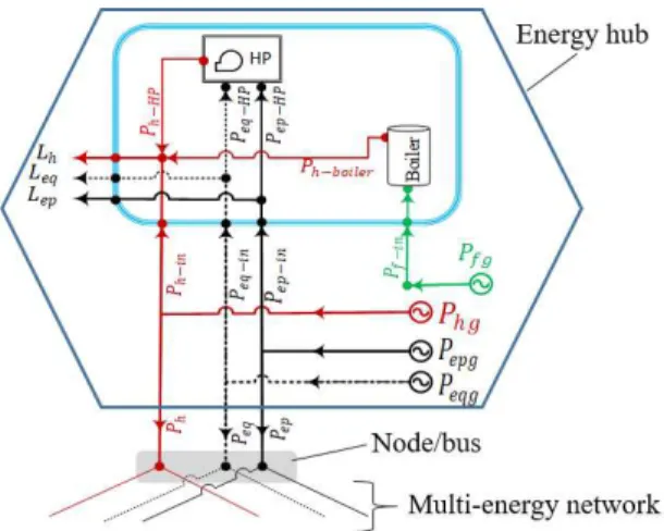
Figure 1 illustrates how electricity, heat and fuel interact inside an energy hub consisting of HP and HOB. By referring Fig 1, the governing equations relating the electricity, heat and fuel in the energy hub consisting of HP and HOB can be expressed in the form of matrices as shown in equation (2).
Fig. 1. Interaction between fuel, heat and electricity in an energy hub consisting of HP and HOB: Pfg, Phg, Pepg and
Peqg are local generations of fuel, heat, active electric and reactive electric power respectively; Ph, Pep and Peq represent the heat, active electric and reactive electric power injections into the network respectively; Ph-in, Pf-in, Pep-in and Peq-Pep-in are the heat, fuel, active electric and reactive electric power Pep-inputs Pep-into the couplPep-ing system respectively; Lh, Lep and Leq are the heat, active electric and reactive electric demands respectively; Ph-boiler and Ph-HP represent the heat power outputs from the gas boiler and HP respectively; Pep-HP and Peq-HP represent the active and reactive electric power consumptions of the HP.
⎣ ⎢ ⎢ ⎢ ⎡ + # ! + # ! $%# &' ( &' − # !∗ * ⎦⎥ ⎥ ⎥ ⎤ = +1 0 0 00 1 0 0 0 0 1 . ⎣ ⎢ ⎢ ⎢ ⎡ −− − ⎦ ⎥ ⎥ ⎥ ⎤ (2)
2.3. Fuel, heat and electricity interaction in HP-CHP energy hub
A waste to energy CHP plant is considered in this study. It produces both active electric power and heat from municipal solid waste. The typical municipal solid waste has a lower heating value of 11MJ/kg [31]. Profitability of waste to energy plants highly depends on the gate fee, which varies from country to country between 10$/ton to 100$/ton [32]. A gate fee of 50$/ton of waste is considered in this study. The performance of a waste to energy CHP is expressed by its electrical ( / and thermal ( 0 ) efficiencies. In this study, a waste to energy CHP plant (with an internal combustion engine) that has an electrical efficiency of 31% and thermal efficiency of 57% is assumed [31]. Depending on whether it is running at lagging or leading power factor ( 1 !), the CHP plant either consumes or produces reactive power. A lagging power factor of 0.9 is assumed.
The interaction between fuel, electricity and heat in an energy hub that has an HP and a CHP is shown in Fig 2. By referring Fig 2, the coupling matrix for an energy hub consisting of HP and CHP is derived as shown in equation (3). In both equations (2) and (3), power factor is considered to be positive if it is lagging and negative otherwise.
Fig. 2. Interaction between fuel, heat and electricity in an energy hub consisting of HP and CHP: Ph-CHP, Pep-CHP and Peq-CHP are the heat, active electric and reactive electric power outputs of a CHP plant.
⎣ ⎢ ⎢ ⎢ ⎡ + # ! + # ! $%# &' ( &' − # !∗ * ⎦⎥ ⎥ ⎥ ⎤ = ⎣ ⎢ ⎢ ⎢ ⎡1 0 0 / 0 1 0 − / $%# 2&'( 2&' 0 0 1 0 ⎦⎥ ⎥ ⎥ ⎤ ⎣ ⎢ ⎢ ⎢ ⎡ −− − ⎦ ⎥ ⎥ ⎥ ⎤ (3)
2.4. Equations governing the electricity network
AC power flow model of an electricity network is used to define the per unit active and reactive power injections at any bus k as a function of all nodal voltages and line parameters, as shown in equations (4a) and (4b) respectively [33].
3 = ∑ |6789% 3|:68:;<38=>?@38+ A38?BC@38D, (4a) 3 = ∑ |6789% 3|:68:;<38?BC@38− A38=>?@38D, (4b)
where @38 is the voltage angle difference between bus k and bus j; <F8+ GAF8 = HF8 is an element of the network admittance matrix (the details on its formation can be referred from [27]); |63| is voltage magnitude at bus k and N is the total number of buses.
A thermo-hydraulic model of the heating network is governed by nodal energy balance, mass balance, pressure drop and temperature drop equations. Equation (5) defines the heat power injection into the network from hub k, 3, as a function of mass flow from the hub, IJ3, and its temperature on the supply and return sides, KL3 and KM3 respectively.
3 = IJ3 KL3− KM3 , (5)
where is specific heat capacity of water.
The mass flow from the hub is subjected to continuity of flow at the corresponding node, which is given by equation (6). In addition, pipe equations are used to relate the pipe flows with the upstream and downstream hydraulic heads as shown in equation (7).
∑ all mass flows into the node3 = ∑ all mass flows out of the node3 (6)
\8− \F= ]F8IJ8F:IJ8F: (7)
where IJ8F is the pipe mass flow from node j (at hydraulic head \8) to node i (at hydraulic head \F) and ]F8 is the corresponding pressure resistance coefficient which (which is further expressed as a function of flow rate and surface roughness [27]).
Thermal energy balance of mixing water at a given node is given by equation (8).
∑;T_#`amJ_#`aD = T_#bcd∑;mJ_#bcdD (8)
where (IJ8#ef0, K8#ef0 terms are the outgoing mass flow rates and water temperature at a given node j while (IJ8#Fg, K8#Fg terms are the incoming mass flow rates and water temperatures at the same node j respectively.
The overall heat transfer coefficient between the water in the pipe and the soil is given by equation (9a) [34] based on which the temperature drop across a pipe is modelled using equation (9b).
h = i jk jl m+ jk 3(nC o j( jlo + jk 3pnC o jp j(o + jk 3knC o jk jpoq #% (9a) Kr_ gt− Ke= ;Kruvwxv− KeDexp {− |}jk~• 1€•J ‚ (9b)
where Kr_ gt and Kr_L0ƒM0 are outlet and inlet water temperatures, respectively. Ke is soil temperature at the surface of the pipe; U is the overall heat transfer coefficient; „%, „|, „…and „† are the inner radius of carrier pipe, outer radius of the carrier pipe, outer radius of an insulation layer and outer radius of an outer jacket, respectively; ℎr, ˆ|, ˆ… and ˆ† represent the convective coefficient of water, thermal conductivity of carrier pipe, thermal conductivity of the insulating material and thermal conductivity of the outer jacket. The convective coefficient of water is function of its flow rate and conductivity [34].
The heat transfer coefficient and the temperature difference between the water and the soil, and the mass flow rate are determinant factors for the heat loss. The supply and return temperatures of a DHN in Stockholm, for example, varies from 60 - 115℃ and 35 - 55℃, respectively [15]. As a result, the relative percentage of heat losses varies throughout a year. The annual average heat loss in Sweden amounts 9.1% of the total heat produced while it reaches up to 21.0% in Lithuania and 27.8% in Korea[35].
2.6. Integrated load flow analysis
Once all the equations are formulated in per unit system the overall load flow problem is solved as a single problem using the Newton-Raphson iteration method (the detailed procedures is found in Ayele et al. [27]). The load flow solution enables us to calculate the distribution of losses in both networks, the voltage profile in the electricity network and temperature and mass flow profiles in the DHN.
The electricity consumption by the circulation pumps to overcome the frictional and local pressure losses in the network as well as to guarantee the minimum pressure difference required between the supply and the return sides of a remote consumer substation is given by equation (10). The first term in equation (10) corresponds to the pressure loss in the network while the second term corresponds to the pressure difference required at consumer substations.
/€‰Š€= 1 + /e‹ ∗ ∑ 2 {
∗:∆ Ž•∗•JŽ•:
• ‚ F L+ ∑ i ∗∆ ‘’“
• |I‹eg|q‹egLf• ML (10)
where /_ f• is active electric power consumed by circulation pumps on each branch in Watt; ” is gravitational acceleration; ∆\F8 is the frictional head loss on a pipe connecting nodes i and j (assuming straight pipe); :IJF8: is magnitude of the mass flow in the pipe and is efficiency of the circulation pump (it is assumed to be 80% in this study). /e‹ is a fraction to take the local pressure losses due to valves and junctions into account while the factor 2 is due to equal pressure drop on both supply and return pipes. ∆\‹eg is the hydraulic head difference at the consumer substation in meter while |I‹eg| is the magnitude of mass flow rate on the primary side of the substation. In this study, the values of /e‹ and ∆\‹eg
are assumed to be 0.3 and 5.1m (≈ 50ˆ —), respectively [36]. It is also assumed that the total electricity consumption of the circulation pumps is very small when compared to the total electrical demand in the system. Hence, their impact on the operational parameters of the electricity network is neglected.
2.7. Optimal placement and sizing of HPs and a HOB
In this study, a novel methodology on optimal placement of HPs and a HOB with the full consideration of both heating and electricity networks is proposed. The objective function is defined by equation (11). The operational cost is the sum of all costs of local generations and imports in both networks including fuels consumed by the coupling devices. It also includes the consumption of circulation pumps. Two scenarios are considered by varying the α value between 0 and 1.
• In Scenario I, the location of HPs is optimized from the point of only heating network without considering the loss in the electricity distribution network (α = 1).
• In Scenario II, both networks are considered in the optimization (α = 0).
IBC™ * š›—œB>C—n >?œ − • >?œ > šnš=œ›B=Bœž ŸB?œ›B ¡œB>C n>?? ¢ (11) For each candidate optimal solution, the load flow equations (2)-(9) are used as equality constraints, which are solved using Newton-Raphson iterative method to determine the operational parameters of both networks. In addition, voltage magnitude, the transmission line capacity ( per conductor) and pipe capacity are defined as inequality constraints as shown in equations (12a)-(12c), respectively. Penalty factors are used for any violation of the constraints. Additional constraints on technology capacity are discussed in section 3.
0.9 ≤ :63 MfgF0: ≤ 1.1 (12a)
0 ≤ :¦F8 M•L: ≤ 480© (12b)
0 ≤ :IJF8: ≤ 9.3 ˆ”/? (12c)
Since the installation of CHP and solar PV plants is site specific, they are assumed to be fixed geographically. The HP and HOB, on the other hand, can be assumed relatively easy to relocate them in the network. Accordingly, only HPs and HOB are considered in the location optimization while all of the solar PV, CHP, HOB and HP are considered in the economical dispatch.
A nested PSO is implemented in this study. The outer PSO is dedicated for optimal placement while the inner PSO determines the corresponding economical dispatch of the HPs and other technologies. PSO is first developed by Kennedy and Eberhart [37] in 1995. It tries to find the global best value in analogy to the way a flock of birds scatter and regroup.
The whole group is referred to as a population (swarm) and its individual members are called particles. If there are M variables of optimization, the position of each particle in the swarm is defined by a point as shown in (13a) which is updated at each iteration using equations (13b) and (13c) [37].
¬F= ¬F%, ¬F|, … , ¬F® (13a)
¯F#g r= °¯Fe+ =%›% ¬F# L0− ¬F + =|›| ¬ # L0− ¬F (13b)
¬F#g r= ¬F+ ¯F#g r (13c)
Where ¬F is the current position of particle i; ¯F#g r is the new velocity of particle i, ° is the inertia/damping factor; ¯Fe is the current velocity of particle i; =% is a self-accelerating factor; =| is a global accelerating factor; ¬F# L0 is the best position of the particle in the past; ¬ # L0 is the global best position achieved by the swarm in the past; ›% and ›| are random numbers between 0 and 1 and ¬F#g r is the new position of particle i.
The flow chart of the nested PSO is shown in Fig 3, which follows the following steps.
i. The network topology, pipe and transmission line data are used as input together with the demand profile of each hub. Generation unit and coupling technologies together with their generation price and capacity constraints are also part of the input data.
ii. Random population of N particles is generated in the outer PSO each of them containing integer values corresponding to the hubs where the HPs and HOB are located. Placement of multiple units at the same hub is possible.
iii. The position of each particle in the outer PSO is updated according to equation (13).
iv. The equations of the integrated load flow model are configured according to the location of HPs and HOB. v. The inner PSO, shown within the broken rectangle in Fig 3, is used to evaluate the fitness of each particle from
the outer PSO loop. A random population of M particles is generated in the inner PSO to find out the best operational sizes of the HPs and HOB together with other generations that have fixed locations.
vi. The position of each particle in the inner PSO are updated according to equation (13).
vii. Integrated load flow is then computed for each particle in the inner PSO loop which is followed by fitness evaluation using equation (11).
viii. The fitness values are compared with the particle’s best fitness and the global best fitness values in the inner PSO. Accordingly, the particle’s best position and the global best position are updated
ix. Steps (vi)-(viii) are computed for each of the M particles in the inner PSO.
x. If the preset maximum iteration of the inner PSO (MaxIter2) is not reached, step (ix) is repeated.
xi. The global best fitness value returned from the inner PSO loop is used as the particle’s fitness value in the outer PSO loop.
xii. This value is used to update the particle’s best and the global best positions in the outer PSO. xiii. Steps (iii)-(xii) are computed for each of the N particles in the outer PSO.
xiv. If the preset maximum iteration of the outer PSO (MaxIter1) is not reached, step (xiii) is repeated.
xv. The best location of the HPs and HOB is contained in the global best position of the outer PSO while their economical dispatch is contained in the corresponding global best position of the inner PSO.
In both of the PSO loops, the global best value is updated after evaluating each particle’s fitness and the latest global best value is used to update the position of the next particle.
Start
End Is Iter1 <
MaxIter1 ?
Initialize population Pop1 of outer PSO with N random particles of possible locations for HPs and HOB
yes
Network topology and coupling-technology parameters,
constraints and load inputs
Configure the load flow model based on the location of HPs and HOB
Initialize population Pop2 of inner PSO with M random particles for economical dispatch of all available generations
Run integrated load flow Evaluate fitness function and update
particle’s best position in Pop2 Update global best position of Pop2
Is j < M ?
j=j+1
Update particle’s position in Pop2 based on the global best and its own best positions
No
Update particle’s best position in Pop1 based on the global best value of Pop2
Update global best position of Pop1
Is i < N ? i=i+1 yes Is Iter2 < MaxIter2 ? No Iter2=Iter2+1 and j=1 yes Update particle’s position in Pop1 based on
the global best and its own best positions
No
yes
No
Iter1=Iter1+1 and i=1
Set maximum iterations for outer PSO as
MaxIter1 and start with Iter1=1, and particle i=1
Set maximum iteration for inner PSO as MaxIter2 and start with Iter2=1, and particle j=1
3. Case studies
Two case studies consisting of heating and electricity networks that are coupled with a waste to energy CHP and HPs In addition solar PV and wind power plants are considered as distributed generations. HOB is also considered as a competitive technology. The optimal placement of the HPs depends the availability of electricity and thermal load. In order to make the optimization problem more challenging, the source of electricity are assumed to be installed at hubs with no thermal demands. The first case study deals with a small part of a distribution network in a densely populated area while the second case study deals with a sparsely populated area connected with a relatively larger network size. The single line diagrams are presented in Figs 4 and 5 with a solid line representing the electricity and the broken line representing the heating network (one line represents both the supply and the return pipes). The hexagons represent energy hubs while the grey circles refer the corresponding node/bus.
3.1. General assumptions
The following assumptions are made for both case studies.
• As the focus of this study is the distribution losses of existing networks, only operational costs are considered.
• The installation of solar PV panels, wind turbines and waste to energy CHP plants are site specific and it is difficult to relocate them. Their locations are assumed to be fixed at certain hubs.
• Hub1 is considered as a slack hub at which any import/export from/to the neighborhood network takes place.
• The price of electricity and heat from the neighborhood is assumed to be 0.2€/kWh and 0.1 €/kWh, respectively.
• A power purchase agreement of 0.12€/kWh for active electric power is considered. As such practical agreement is not yet fully developed for heating networks, it is neglected.
• A reactive power penalty of 0.02€/kvarh is considered for the imported reactive electric power at the slack hub in excess of 48.5% (corresponding to a 0.9 lagging power factor) of the imported active electric power.
• The price of gas used in the HOB is taken to be 0.113/kWh. The HOB thermal efficiency is 90%.
• Operating cost of the waste to energy CHP plant is assumed to be -0.016€/kWh which corresponds to a gate fee of 50 €/ton of waste with an average heating value 11MJ/kg.
• The thermal and electrical efficiencies of the waste to energy plant are assumed to be 57% and 31%, respectively at a lagging power factor of 0.9.
• The operating cost of solar PV is assumed to be negligible.
• All HPs are assumed to run at a COP of 4.0 and a lagging power factor of 0.9.
• The electricity network is assumed to be balanced three phase system. All transmission lines are assumed to be three phase ACSR Waxwing type with resistance, reactance, susceptance and ampacity of 0.262Ω/km, 0.386Ω/km, 4.31µS/km and 480A, respectively [38]. Double conductors are used between hubs 1 and 2.
• All pipes in the DHN are of DN-100 type with standard insulation layer. The parameters (carrier pipe thickness and outer diameter of 3.6mm and114.3mm, and outer jacket thickness and outer diameter of 3.2mm and of 200mm, respectively) are taken from isoplus® [39]. Maximum allowed flow rate in the pipe is 9.3kg/s. Thermal
conductivity of the carrier pipe, outer jacket and insulation material are 40W/mK, 0.4W/mK and 0.027W/mK, respectively. Surface roughness of the carrier pipe is assumed to be 0.05mm.
• The water in the DHN pipes is assumed to be incompressible with constant density (982.6kg/m3), specific heat
• All hubs acting as a heat source are assumed to have a supply temperature of 70℃ and all hubs acting as a heat consumer are assumed to have a return temperature of 50℃ on the network side. A uniform soil temperature of 4.36℃ is assumed around the supply and return pipes of the DHN.
• Both residential and commercial demands are considered. Peak demand of one/two residential buildings and a small hotel located in Idaho, USA are taken as a reference from an Open Energy Information database
[40]
. An electrical power factor of 0.95 and 0.9 lagging is assumed for residential and commercial demands, respectively.3.2. Specific inputs for Case 1
A small distribution network topology for Case 1 is shown in Fig 4. The load distributions are summarized in Table 1. The CHP with a maximum of 200kW waste intake capacity is installed at Hub3. A solar PV with 50kW output is connected at Hubs 5. The electricity distribution network is at 0.4kV. Two heat pumps, each of which are rated at 25kWe, and a HOB that can take up to 30kW of gas are considered in the optimization. In order to find their optimal placement in the network and their economical dispatch, a swarm of 5 particles with 15 iterations is considered in the outer PSO, while a swarm with 10 particles and 70 iterations is used in the inner loop.
2 3 Electricity network Heating network 4 6 1 2 3 4 5 6 10m Energy hub Node/bus Solar PV
Fig. 4. One line diagram of the heating and electricity network considered for Case 1. Table 1: Load distribution for Case 1
Hubs Hub1 Hub2 Hub3 Hub4 Hub5 Hub6 Total Active electric power demand (kW) 0 67.1 0 134.21 0 199.5 400.81 Reactive electric power demand (kvar) 0 22.08 0 44.16 0 96.56 162.8 Heat demand (kW) 0 77.09 0 154.19 0 54.64 285.92
3.3. Specific inputs for Case 2
A relatively larger and sparsely populated distribution network topology for Case 2 is shown in Fig 5. The load distributions are summarized in Table 2. The CHP is assumed to be installed at Hub2 and its maximum waste intake capacity is 3MW. A wind power plant with 1MW active electrical output is connected at Hub26. The electricity distribution network is at 4.16kV except part of the network after buses 7, 19 and 27 which is at 0.4kV. Step down transformers (4.16kV/0.4kV) with 0.9-1.1 tap setting are installed near to the buses 7, 19 and 27, as shown in Fig 5. The tap settings are set to 0.9 to improve the voltage profile in the 0.4kV distribution network. Four heat pumps, each of which are rated at 100kWe, and a HOB that can take up to 100kW of gas are considered in the optimization. In order to find their optimal placement in the network and their economical dispatch, a swarm of 10 particles with 30 iterations is considered in the outer PSO, while a swarm with 15 particles and 70 iterations is used in the inner PSO.
2 1 2 11 3 10m 300m 24 26 26 13 27 28 28 29 29 25 25 12 12 14 14 15 15 300m 300m 16 17 17 18 18 300m 300m 19 20 20 22 22 300m 300m 21 21 300m 7 8 8 9 9 300m 300m 10 10 300m 4 6 6 300m 5 5 300m 23 23 300m 300m 300m 300m 300m 300m 300m 300m 300m 300m 300m 300m 3 13 11 24 27 7 16 4 19 300m Electricity network Heating network Energy hub Node/bus 300m 300m 4.16kV/0.4kV transformer Wind power plant
Fig. 5. One line diagram of a 29 hub coupled heating and electricity network considered for Case 2. Table 2: Load distribution for Case 2
Hub1 Hub2 Hub3 Hub4 Hub5 Hub6 Hub7 Hub8 Hub9 Hub10 Active electric power demand (kW) 0 0 134.21 134.21 134.21 134.21 0 134.21 134.21 134.21 Reactive electric power demand (kvar) 0 0 44.16 44.16 44.16 44.16 0 44.16 44.16 44.16
Heat demand (kW) 0 0 154.18 154.18 154.18 154.18 0 154.18 154.18 154.18 Hub11 Hub12 Hub13 Hub14 Hub15 Hub16 Hub17 Hub18 Hub19 Hub20 Active electric power demand (kW) 134.21 134.21 0 199.5 199.5 199.5 199.5 199.5 0 134.21 Reactive electric power demand (kvar) 44.16 44.16 0 96.56 96.56 96.56 96.56 96.56 0 44.16
Heat demand (kW) 154.18 154.18 0 54.64 54.64 54.64 54.64 54.64 0 154.18 Hub21 Hub22 Hub23 Hub24 Hub25 Hub26 Hub27 Hub28 Hub29 Total Active electric power demand (kW) 134.21 134.21 134.21 134.21 134.21 0 199.5 134.21 134.21 3478.6
Reactive electric power demand (kvar) 44.16 44.16 44.16 44.16 44.16 0 96.56 44.16 44.16 1330.1
Heat demand (kW) 154.18 154.18 154.18 154.18 154.18 0 54.64 154.18 154.18 2948.9
4. Results and discussion
4.1. Optimization results for Case 1
The optimal locations of the two HPs and the HOB together with their operating size and the resulting distribution of losses are summarized in Table 3. Imported powers for each energy carrier are also given in the same table. Although the highest heat demand is at Hub4, the optimal location of the HPs in Scenario I are found to be at Hubs 2 and 6. This is due to the existence of a cheap heat source from the CHP plant at Hub3 which has no other connection other than Hub4. In scenario II, on the other hand, the HPs are placed at Hub2 instead of Hub3 or Hub5 where there is cheap electricity generation. The reason is the existence of heat demand at Hub2 and due to the fact that larger proportion of the active electricity comes from the slack hub (see Table 3). In both scenarios, the CHP and solar PV are selected at their maximum output followed by HPs. No HOB is selected. Importing heat is also found to be expensive relative to the heat from HPs. The results for both scenarios shows that the optimal placement of HPs is not aligned with active electricity generation hubs (hubs 1, 3 and 5). They are, rather, placed at some of the hubs where there is heat demand. In scenario I, 54.6% of the total heat generated (290.5kW) is transported in the heating network while 100% of the total active electricity generated (462.38kW) is transported in the electricity network. In the case of scenario II, however, 73.55% of the total heat generated (291.3kW) and 100% of total active electricity generation (459.52kW) is transported in the corresponding networks. As a result, scenario I has lower heat loss (1.6% of the heat demand) than Scenario II (1.9% of the heat demand).
The active electric power loss, on the other hand, is higher (3.9% of the demand including HPs’ consumption) for Scenario I than Scenario II (3.2% of the demand including HPs’ consumption).
The pumping power required for circulation in scenarios I and II are 0.12kW and 0.16kW respectively, which are negligible relative to the total electricity demand. It is also found that only 0.05% and 0.07% of this pumping energy is used to overcome the friction and local pressure losses in the network respectively while the remaining is used to keep the pressure drop at the consumer substations. The cost of pumping energy for scenarios I and II is 0.024€/h and 0.032€/h which are less significant compared with the corresponding cost of heat loss (0.46€/h and 0.54€/h respectively). This is in agreement with the findings of [12] but in disagreement with the findings of [36]. The possible reasons could be the difference in the pipe parameters (diameter, length etc.) and operational strategies. The operating cost of the whole network is 68.3€/h in scenario I. This value is reduced to 67.68€/h in scenario II which shows nearly 1% saving. This is due to the fact that the price of electricity is twice of the heat if they are compared at the importing level. The difference grows to even four times if the heat from the HPs is considered.
Table 3: Optimal location and generation of different energy carriers from different energy technologies in Case 1
Scenarios Energy carrier HPs HOB CHP PV Imported Loss
I
Location (hub numbers) 2 6 4 3 5 1 total Active electricity (kW) -19.45 -24.67 0.00 62.00 50.00 350.38 17.45 Reactive electricity (kvar) -9.42 -11.95 0.00 -30.03 0.00 239.90 25.71 Heat (kW) 77.80 98.68 0.00 114.00 0.00 0.00 4.58
II
Location (hub numbers) 2 2 6 3 5 1 total Active electricity (kW) -25.00 -19.33 0.00 62.00 50.00 347.52 14.37 Reactive electricity (kvar) -12.11 -9.36 0.00 -30.03 0.00 235.47 21.17 Heat (kW) 100.00 77.32 0.00 114.00 0.00 0.00 5.38
Figure 6 depicts the temperature and mass flow profiles at different hubs. A positive mass flow implies that the hub is acting as a source of heat. Hub6, for example, is acting as a source in Scenario I and as a consumer in Scenario II. When the mass flow from the hub is closer to zero, the water gets more time to lose its heat and, as a results, its temperature gets closer to the soil temperature (for example the return temperature at Hub2 in Scenario I). If the mass flow is zero, as in the case for Hub5 in both scenarios, the steady state temperature of water on both the return and supply pipes becomes equal to the soil temperature.
(a) (b)
Fig. 6. a) The mass flow injected into the network from each hub and b) the corresponding supply and return temperatures for the two scenarios of Case 1.
M a ss flo w fr o m h u b ( kg /s) T e m p e ra tu re ( oC)
The pipe mass flows are shown in Fig 7. All the flows are within the acceptable range of 9.3kg/s defined in equation (12c). Negative flow for Pipe4-6 implies that the flow is opposite to the initially assumed positive flow direction (i.e. from 4 to 6).
Fig. 7. Mass flow in the pipes for two scenarios of Case 1
(a) (b)
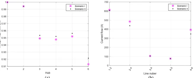
Fig. 8. a) Voltage profiles at different hubs and b) phase currents through the transmission lines for the two scenarios of Case 1
The voltage magnitude profiles, as shown in Fig 8(a), are within the limits of equation (12a). Scenario II has a relatively better voltage profile. The root mean square current through each transmission line are illustrated in Figs 8(b). It looks that the current in Line1-2 is above the acceptable limit of 480A. But, since double conductors are assumed for each phase, the current in each conductor is still in the acceptable range. It also shows that the current in Line2-4 in Scenario I is 484.5A which slightly higher than the acceptable limit. It means that optimizing HPs without the consideration of electricity network constraints (as is the case for Scenario I) could lead to overloading of the electrical distribution network.
4.2. Optimization results for Case 2
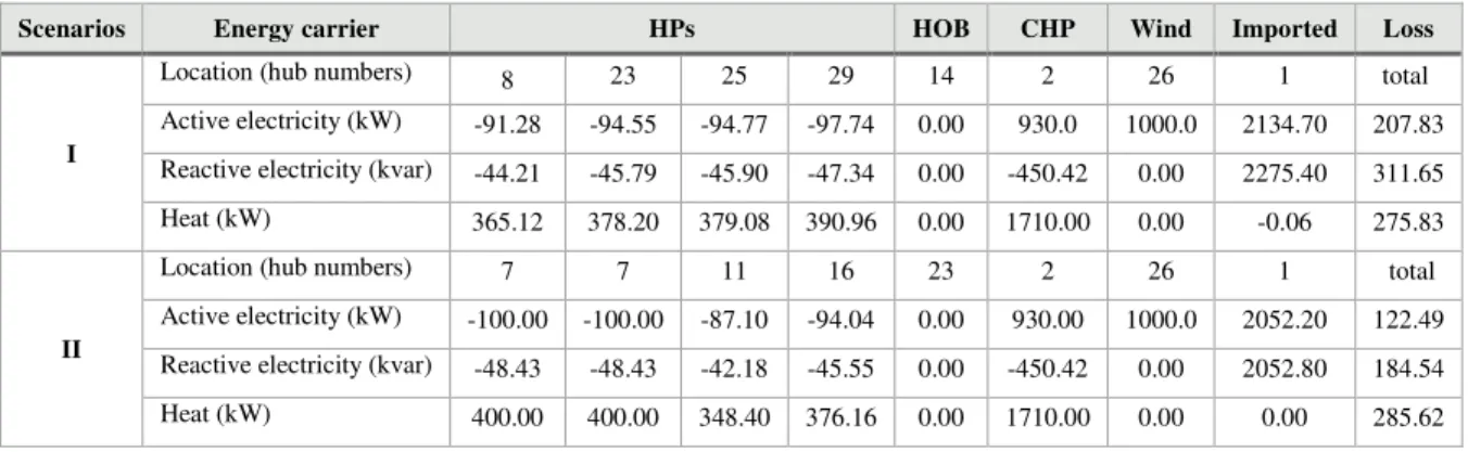
Table 4 presents the optimal location and operational sizes of the HPs, HOB together with the economical dispatches of CHP and wind plants. It also shows the distribution losses and amount of import for each energy carrier. The full capacity of the CHP and the wind power plants are selected in both scenarios. The remaining electricity is imported from the neighborhood grid while the remaining heat is generated using HPs. Similar to Case 1, HOB and the neighborhood DHN are avoided. 1-2 2-4 3-4 4-5 4-6 M a s s f lo w i n t h e p ip e s ( k g /s ) 1-2 2-4 3-4 4-5 4-6
Similar to Case 1, hubs with electricity generation (hubs 1, 2 and 26) are not selected for optimal placement of the HPs. This is again due to the absence of thermal loads at those hubs. However, as it can be referred from Table 4 and Fig 5, the HPs in scenario II are closer to the hubs with electricity generation when compared to the HPs in scenario I. In scenario I, 53.03% of the total heat generated (3.22MW) is transported in the heating network while 100% of the total active electricity generated (4.06MW) is transported in the electricity network. In the case of scenario II, however, 93.55% of the total heat generated (3.23MW) and 100% of total active electricity generation (3.98MW) is transported in the corresponding networks.
The heat loss in the distribution network for Scenarios I and II are 9.35% and 9.69% of the heat demand, while the active electricity losses are 5.39% and 3.17% of the electricity consumption, respectively. Compared with Case 1, the losses are higher which is partly due to longer branches and larger percentage of power flows in the network. Table 4 also shows that, although the increase in the heat loss from scenario I to II is not significant, the reduction in the electricity loss is tremendous, which is 41.2%. This can be explained by considering the way HPs are installed. In Scenario I the HPs are placed at the farthest nodes relative to the CHP plant. Nodes 8, 23 and 29 belong to the 0.4kV distribution network while node 25 belongs to the 4.16kV distribution network. On the other hand, all of the four HPs are installed at 4.16kV nodes in Scenario II. The current drown by the HPs at the 0.4kV node is equal to the amount of current it could draw at 4.16kV multiplied by the transformer ratio. The more current flowing in the network, the more the losses.
The pumping power required for circulation in scenarios I and II are 3.79kW and 5.3kW respectively, which are negligible relative to the total electricity demand. Unlike to Case 1, about 50.73% and 59.06% of this pumping energy is used to overcome the friction and local pressure losses in the network respectively which are significant. However, the costs of the pumping energy are still insignificant when they are compared to the cost of heat lost (2.74% and 3.71% considering the importing prices of heat and electricity). The operational cost is 404.5€/h for Scenario I while it is 384.65€/h for Scenario II which shows about 5% reduction. It means that a relatively larger saving can be achieved for larger networks by applying an integrated optimization rather than considering only heating network.
It is important to note that nodes 9 and 10 in Fig 5 are equally optimal as node 8 due to the symmetry in the network dimension and demands at the nodes (see Table 2). This applies to other symmetrical nodes too. The more asymmetry in the network, the faster the PSO gets to the global optimal solution.
Table 4: Optimal location and generation of different energy carriers from different energy technologies in Case 2
Scenarios Energy carrier HPs HOB CHP Wind Imported Loss
I
Location (hub numbers) 8 23 25 29 14 2 26 1 total Active electricity (kW) -91.28 -94.55 -94.77 -97.74 0.00 930.0 1000.0 2134.70 207.83 Reactive electricity (kvar) -44.21 -45.79 -45.90 -47.34 0.00 -450.42 0.00 2275.40 311.65 Heat (kW) 365.12 378.20 379.08 390.96 0.00 1710.00 0.00 -0.06 275.83
II
Location (hub numbers) 7 7 11 16 23 2 26 1 total Active electricity (kW) -100.00 -100.00 -87.10 -94.04 0.00 930.00 1000.0 2052.20 122.49 Reactive electricity (kvar) -48.43 -48.43 -42.18 -45.55 0.00 -450.42 0.00 2052.80 184.54 Heat (kW) 400.00 400.00 348.40 376.16 0.00 1710.00 0.00 0.00 285.62
Figure 9 shows the nodal mass injection from each hub and the corresponding temperature profiles on the supply and return pipes. The nodal mass flows for both scenarios lookalike for all nodes except where the HPs are installed (Fig 9(a)). Hubs with no heat consumption and production, for example 13, 19 and 26, can be treated as either sources or consumer in the numerical computation depending on the direction of mass flow obtained from the load flow solution. The mass flow always is zero at these hubs. However, the temperature can vary depending on the assumption. In any case, the heat power injected into the network is zero and the mass and temperature balances at the mixing nodes are
always guaranteed. Hub13, for instance, is considered as a source in Scenario I in which its supply temperature is fixed at 70℃. Its return temperature is equal to the outgoing return temperature of the mixing at Node13. On the other hand, Hub13 is treated as a consumer in Scenario II in which case the return temperature is assumed to be equal to the soil temperature as there is no flow. The supply temperature will then be equal to the outgoing supply temperature of the mixing at Node13. Hub19 is treated as a source in both scenarios.
(a) (b)
Fig. 9. a) The mass flow injected into the network from each hub and b) the corresponding supply and return temperatures for the two scenarios of Case 2.
The pipe flows are depicted in Fig 10. All pipe flows are within the acceptable range of 9.3kg/s. The voltage profiles at each hub and the current through each transmission lines are shown in Fig 11. The current flows are also below the limit of 480A. However, there voltage magnitudes at Hubs8 and 29 are below the acceptable voltage of 0.9pu. These nodes belong to the 0.4kV distribution network. Although the nearby transformers are set at the lowest possible tap setting of 0.9, they are not enough to keep the voltage above 0.9pu. The voltage profiles in Scenario II, however, are within the acceptable range of 0.9 -1.1pu.
Fig. 10. Mass flow in the pipes for the two scenarios of Case 2
(a) (b)
Fig. 11. a) Voltage profiles at different hubs and b) phase currents through the transmission lines for the two scenarios of Case 2 T e m p e ra tu re ( oC ) 1-2 2-32-11 2-1 3 3-4 3-7 4-5 4-6 7-8 7-97-10 11-1 2 11-2 4 24 -25 24 -26 26 -27 27 -28 27 -29 13 -14 13 -15 13 -16 16 -17 16 -18 16 -19 19 -20 19 -21 19 -22 19 -23 Pipe number -4 -2 0 2 4 6 8 10 M a s s f lo w i n t h e p ip e s ( k g /s ) Scenario I Scenario II V o lt a g e m a g n it u d e ( p u ) 1-22-32-112-133-43-74-54-67-87-97-109-23 11-1 2 11-2 4 24-2 5 24-2 6 13-1 4 13-1 5 13-1 6 16-1 7 16-1 8 16-1 9 16-2 6 19-2 0 19-2 1 19-2 2 19-2 3 26-2 7 27-2 8 27-2 9 Line 0 50 100 150 200 250 300 350 400 450 Scenario I Scenario II
In this paper, a nested PSO algorithm, integrated with the load flow model based on an extended energy hub, is proposed to find out the optimal location and sizes of distributed generation and coupling technologies. Two case studies of coupled heating and electricity networks consisting of a CHP, HOB, HPs, Solar PV and wind power plant are considered. The HPs are found to be more economical than the neighborhood DHN and a HOB for the given price data. The results show that optimizing the location and sizes of HPs only from the heating network point of view could lower the heat loss, but sometimes it could overload and increase the loss in the electricity distribution network, especially when HPs are installed at very low voltage distribution networks. It could also lead to unacceptable voltage profiles. On the other hand, an integrated optimization which considers the constraints and distribution losses in both networks results in a lower operational cost for the overall system with the possibility of better voltage profile in the electricity network. It is also observed that the electricity consumption of circulation pumps is not significant compared to the total electricity demand. However, the cost might become significant compared to the cost of heat lost specially when there are cheap heat sources in the network. It is observed that the frictional pressure losses are equally important as the pressure losses at the consumer substations for larger networks. Hence, it might be worthy to consider the total cost of pumping energy in thermo-economic optimizations of large networks.
The methodology presented in this paper is a step forward in optimization of integrated energy systems. It can be applied to different MES consisting of different distributed generations and coupling technologies. It can be further complemented by considering time series data for solar PV and wind power generation together with thermal storage units. Once the optimal locations of coupling technologies are identified, additional optimization variables such as temperature and transformer tap setting can be incorporated. The methodology can also be applied for future energy systems at planning phase in which case the investment cost of the network and coupling technologies will be taken into account. Other optimization algorithms can also be applied and compared with.
Acknowledgments
The research presented is performed within the framework of the Erasmus Mundus Joint Doctorate SELECT+ program ‘Environomical Pathways for Sustainable Energy Services’ and funded with support from the Education, Audiovisual, and Culture Executive Agency (EACEA) (FPA-2012-0034) of the European Commission. This publication reflects the views only of the author(s), and the Commission cannot be held responsible for any use, which may be made of the information contained therein.
Nomenclature Letter symbols
C coupling coefficient
Cp specific heat capacity of water (J/Kk) CHP combined heat and power
COP coefficient of performance DHN district heating network H hydraulic head (m) HP heat pump HOB heating only boiler
K pressure resistance coefficient (m.s2/kg2)
Lep electricity active power demand (W)
Leq electricity reactive power demand (var)
Lh heat power demand (W)
IJ mass flow rate from a hub (kg/s) IJF8 mass flow rate from node i to j (kg/s)
MES multi energy system
Pep electricity active power injection (W)
Pepg electricity active power generation (W)
Peq electricity reactive power injection (var)
Peqg electricity reactive power generation (var)
Pf fuel power injection (W)
Pfg fuel power generation/used (W) 1 ! power factor of a CHP plant
! power factor of an HP Ph heat power injection (W)
Phg heat power generation (W)
T temperature (K) V voltage magnitude (V) Y bus admittance matrix
∆ change
@ voltage angle (degree)
Subscripts
i,j,k hub numbers r return pipe of a DHN s supply pipe of a DHN
References
[1] Mancarella P. MES (multi-energy systems): An overview of concepts and evaluation models. Energy 2014;65:1–17. doi:10.1016/j.energy.2013.10.041.
[2] Lund H, Duic N, Østergaard PA, Mathiesen BV. Future district heating systems and technologies: On the role of smart energy systems and 4th generation district heating. Energy 2018;165:614–9. doi:10.1016/j.energy.2018.09.115.
[3] Commission launches plans to curb energy use in heating and cooling - Energy - European Commission. Energy n.d. /energy/en/news/commission-launches-plans-curb-energy-use-heating-and-cooling (accessed December 30, 2018).
[4] Directive 2012/27/EU of the European Parliament and of the Council of 25 October 2012 on energy efficiency, amending Directives 2009/125/EC and 2010/30/EU and repealing Directives 2004/8/EC and 2006/32/EC Text with EEA relevance. vol. OJ L. 2012.
[5] Lund H, Werner S, Wiltshire R, Svendsen S, Thorsen JE, Hvelplund F, et al. 4th Generation District Heating (4GDH): Integrating smart thermal grids into future sustainable energy systems. Energy 2014;68:1–11. doi:10.1016/j.energy.2014.02.089.
[6] Widl E, Jacobs T, Schwabeneder D, Nicolas S, Basciotti D, Henein S, et al. Studying the potential of multi-carrier energy distribution grids: A holistic approach. Energy 2018;153:519–29. doi:10.1016/j.energy.2018.04.047.
[7] Ma T, Wu J, Hao L, Lee W-J, Yan H, Li D. The optimal structure planning and energy management strategies of smart multi energy systems. Energy 2018;160:122–41. doi:10.1016/j.energy.2018.06.198. [8] Yammani C, Maheswarapu S, Matam SK. A Multi-objective Shuffled Bat algorithm for optimal placement
and sizing of multi distributed generations with different load models. International Journal of Electrical Power & Energy Systems 2016;79:120–31. doi:10.1016/j.ijepes.2016.01.003.
[9] Kansal S, Kumar V, Tyagi B. Hybrid approach for optimal placement of multiple DGs of multiple types in distribution networks. International Journal of Electrical Power & Energy Systems 2016;75:226–35. doi:10.1016/j.ijepes.2015.09.002.
[10] Pazouki S, Mohsenzadeh A, Ardalan S, Haghifam MR. Optimal place, size, and operation of combined heat and power in multi carrier energy networks considering network reliability, power loss, and voltage profile. Transmission Distribution IET Generation 2016;10:1615–21. doi:10.1049/iet-gtd.2015.0888.
[11] Marguerite C, Bourges B, Lacarrière B. Application of a District Heating Network (dhn) Model for an Ex-Ante Evaluation to Support a Multi-Sources Dh. Proceedings of BS2013, Chambéry, France: 2013. [12] Vesterlund M, Toffolo A, Dahl J. Optimization of multi-source complex district heating network, a case
study. Energy 2017;126:53–63. doi:10.1016/j.energy.2017.03.018.
[13] Shabanpour-Haghighi A, Seifi AR. Simultaneous integrated optimal energy flow of electricity, gas, and heat. Energy Conversion and Management 2015;101:579–91. doi:10.1016/j.enconman.2015.06.002. [14] Allegrini J, Orehounig K, Mavromatidis G, Ruesch F, Dorer V, Evins R. A review of modelling approaches
and tools for the simulation of district-scale energy systems. Renewable and Sustainable Energy Reviews 2015;52:1391–404. doi:10.1016/j.rser.2015.07.123.
[15] Levihn F. CHP and heat pumps to balance renewable power production: Lessons from the district heating network in Stockholm. Energy 2017. doi:10.1016/j.energy.2017.01.118.
[16] Arnaudo M, Zaalouk OA, Topel M, Laumert B. Techno-economic Analysis Of Integrated Energy Systems At Urban District Level – A Swedish Case Study. Energy Procedia 2018;149:286–96. doi:10.1016/j.egypro.2018.08.229.
[17] Geidl M, Koeppel G, Favre-Perrod P, Klockl B, Andersson G, Frohlich K. Energy hubs for the future. IEEE Power and Energy Magazine 2007;5:24–30. doi:10.1109/MPAE.2007.264850.
[18] Aghamohamadi M, Samadi M, Rahmati I. Energy generation cost in multi-energy systems; an application to a non-merchant energy hub in supplying price responsive loads. Energy 2018;161:878–91. doi:10.1016/j.energy.2018.07.144.
[19] Carpaneto E, Lazzeroni P, Repetto M. Optimal integration of solar energy in a district heating network. Renewable Energy 2015;75:714–21. doi:10.1016/j.renene.2014.10.055.
[20] Gabrielli P, Gazzani M, Martelli E, Mazzotti M. Optimal design of multi-energy systems with seasonal storage. Applied Energy 2018;219:408–24. doi:10.1016/j.apenergy.2017.07.142.
[21] Rakipour D, Barati H. Probabilistic optimization in operation of energy hub with participation of renewable energy resources and demand response. Energy 2019;173:384–99. doi:10.1016/j.energy.2019.02.021. [22] Awad B, Chaudry M, Wu J, Jenkins N. Integrated optimal power flow for electric power and heat in a
MicroGrid. CIRED 2009 - 20th International Conference and Exhibition on Electricity Distribution - Part 1, 2009, p. 1–4.
[23] Liu X, Wu J, Jenkins N, Bagdanavicius A. Combined analysis of electricity and heat networks. Applied Energy 2016;162:1238–50. doi:10.1016/j.apenergy.2015.01.102.
[24] Liu X, Mancarella P. Modelling, assessment and Sankey diagrams of integrated electricity-heat-gas networks in multi-vector district energy systems. Applied Energy 2016;167:336–352.
[25] Shabanpour-Haghighi A, Seifi AR. An Integrated Steady-State Operation Assessment of Electrical, Natural Gas, and District Heating Networks. IEEE Transactions on Power Systems 2016;31:3636–47. doi:10.1109/TPWRS.2015.2486819.
[26] Boulos PF, Lansey KE, Karney BW. Comprehensive Water Distribution Systems Analysis Handbook for Engineers and Planners. American Water Works Assn; 2006.
[27] Ayele GT, Haurant P, Laumert B, Lacarrière B. An extended energy hub approach for load flow analysis of highly coupled district energy networks: Illustration with electricity and heating. Applied Energy 2018;212:850–67. doi:10.1016/j.apenergy.2017.12.090.
[28] Østergaard PA, Andersen AN. Booster heat pumps and central heat pumps in district heating. Applied Energy 2016;184:1374–88. doi:10.1016/j.apenergy.2016.02.144.
[29] Bach B, Werling J, Ommen T, Münster M, Morales JM, Elmegaard B. Integration of large-scale heat pumps in the district heating systems of Greater Copenhagen. Energy 2016;107:321–34. doi:10.1016/j.energy.2016.04.029.
[30] Averfalk H, Ingvarsson P, Persson U, Gong M, Werner S. Large heat pumps in Swedish district heating systems. Renewable and Sustainable Energy Reviews 2017;79:1275–84. doi:10.1016/j.rser.2017.05.135. [31] Aracil C, Haro P, Fuentes-Cano D, Gómez-Barea A. Implementation of waste-to-energy options in
landfill-dominated countries: Economic evaluation and GHG impact. Waste Management 2018;76:443–56. doi:10.1016/j.wasman.2018.03.039.
[32] Rezaei M, Ghobadian B, Samadi SH, Karimi S. Electric power generation from municipal solid waste: A techno-economical assessment under different scenarios in Iran. Energy 2018;152:46–56. doi:10.1016/j.energy.2017.10.109.
[33] Glover JD, Sarma MS, Overbye T. Power System Analysis & Design, SI Version. Cengage Learning; 2012. [34] Bergman TL, Incropera FP, DeWitt DP, Lavine AS. Fundamentals of heat and mass transfer. John Wiley &
Sons; 2011.
[35] Danielewicz J, Śniechowska B, Sayegh MA, Fidorów N, Jouhara H. Three-dimensional numerical model of heat losses from district heating network pre-insulated pipes buried in the ground. Energy 2016;108:172– 84. doi:10.1016/j.energy.2015.07.012.
[36] Wang H, Duanmu L, Li X, Lahdelma R. Optimizing the District Heating Primary Network from the Perspective of Economic-Specific Pressure Loss. Energies 2017;10:1095. doi:10.3390/en10081095. [37] Kennedy J, Eberhart R. Particle swarm optimization. Proceedings of ICNN’95 - International Conference
on Neural Networks, vol. 4, 1995, p. 1942–8 vol.4. doi:10.1109/ICNN.1995.488968.
[38] Grigsby LL. Electric Power Generation, Transmission, and Distribution. CRC Press; 2018. doi:10.1201/9781315222424.
[39] isoplus: Flexible and rigid pipes and pipeline systems: isoplus - isoplus Fernwärmetechnik n.d. http://www.isoplus-pipes.com/ (accessed September 3, 2017).
[40] Open Energy Information: Commercial and residential hourly load profile n.d. https://openei.org/datasets/files/961/pub/ (accessed January 8, 2018).